Review

Investigating the Impact of Energy Source Level on the Self-Guided Vehicle System Performances, in the Industry 4.0 Context

Research Chair of Noovelia for Intelligent Navigation of Industrial Autonomous Vehicle, Hydrogen Research Institute, Université du Québec à Trois-Rivières, Trois-Rivières, QC G9A 5H7, Canada
*
Authors to whom correspondence should be addressed.
Sustainability 2020, 12(20), 8541; https://doi.org/10.3390/su12208541
Submission received: 12 September 2020 / Revised: 7 October 2020 / Accepted: 14 October 2020 / Published: 15 October 2020
(This article belongs to the Special Issue Industry 4.0 and Industrial Sustainability)

Abstract

:
Automated industrial vehicles are taking an imposing place by transforming the industrial operations, and contributing to an efficient in-house transportation of goods. They are expected to bring a variety of benefits towards the Industry 4.0 transition. However, Self-Guided Vehicles (SGVs) are battery-powered, unmanned autonomous vehicles. While the operating durability depends on self-path design, planning energy-efficient paths become crucial. Thus, this paper has no concrete contribution but highlights the lack of energy consideration of SGV-system design in literature by presenting a review of energy-constrained global path planning. Then, an experimental investigation explores the long-term effect of battery level on navigation performance of a single vehicle. This experiment was conducted for several hours, a deviation between the global trajectory and the ground-true path executed by the SGV was observed as the battery depleted. The results show that the mean square error (MSE) increases significantly as the battery’s state-of-charge decreases below a certain value.

1. Introduction

Automated Guided Vehicles (AGVs) have transformed the way we conceive of the transportation of materials. Commercially introduced in the early 1950s, their main task was for intralogistics application [1]. This includes production-to-assembly transfers, warehouse picking and depositing and pharmaceutical supply, among others. Although they are considered to have a high initial investment, they reduce labor costs, improve operational flow and dramatically increase production rates. First AGVs were implemented with primitive devices, and the early guidance system used are tactile sensor-based embedded on or in the floor, such as conductors, optical guides, or magnetic tape, allowing the vehicle to move only in restricted areas [1]. Therefore, the performances of the vehicle, such as speed and safety, are limited.
The recent advances in sensors and control systems have permitted the integration of complex robotic concepts in industrial applications [2]. Laser scanning sensors are used as range finders for long distance measuring with high frequency and a resolution that allows for building a detailed map of the environment. From a safety aspect, the scanners can detect obstacles (i.e., workers, furniture, other mobile platforms, machines, etc.) from several meters, which allows the vehicles to safely navigate with a higher speed. Laser scanners combined with other types of sensors provide a better understanding of the surroundings. Therefore, a Self-Guided Vehicle can reach higher guidance level, and is able to freely navigate from places that an AGV cannot; this is referred to as mobile navigation. A navigation is said to be “natural”, which is when it is capable to navigate autonomously and react to situations in a very short time with self-sufficient sensor data, and in any navigable space of a real environment [3].
Today, the problematic goes beyond technology type, the hardware design has gained enough maturity to be industrialized on a large scale. The issue, however, deals with the system efficiency to improve productivity. In this context, Industry 4.0 was introduced at the Hannover Fair in the beginning of the last decade [4]. Described as the fourth industrial revolution, it gives rise to new types of management to enhance different system levels. Some of the aspects that the Smart Factory paradigm is introducing are: digitization, Human-to-Machine (H2M) interactions and Machine-to-Machine (M2M) communication enhancement, flow optimization, adaptability, flexibility, and sustainability [5]. Sustainability is the least addressed issue in literature and the potential impact is still unknown. Nowadays, the need for energy-efficient vehicles has reached an unprecedented necessity [6,7].
Human-Machine-Infrastructure communication, which is defined as Internet-of-Things (IoT) has been a turning point toward Smart Factory [8,9]. The link between the IoT and energy management has also been extensively studied in [8,10]. Indoor logistics systems are being enhanced since the advent of industry 4.0. AGV-System is a freight system that is responsible for managing a set of AGVs used for material handling. This system is becoming more intelligent and more flexible thanks to the cutting-edge connectivity, but also the autonomous navigation capabilities of Self-Guided Vehicle (SGVs).
The object of this paper is to bring an overview of the link that exist between the SGVs navigation system performance and the battery source depletion, in the context of smart factory challenges. Figure 1 shows the focus of this paper. Thus, optimal path planning solutions, as part of mobile navigation, are first reviewed. Then, in order to prove the link between the energy level and the navigation sustainability and assess the necessity improving resource management, an experiment was carried out with an SGV. Hundreds of meters have been traveled and pose data were collected in real-time. Finally, the data have been analyzed and compared with the evolution of the battery level.
This paper is organized as follows: The current section introduces the general context and states the problematic of the paper. Section 2 presents the specific context and the challenges of the SGV-system. The state-of-the-art of global path and trajectory planning and the scope of the work are presented in Section 3. Section 4 reviews the work on energy-constrained trajectory. Section 5 demonstrates the experimental investigation and discusses the effect of low battery on the navigation. We conclude on the investigation results in Section 6.

2. Context

Material Handling System (MHS) for indoor transportation application has always been an inefficient task in any type of facilities. Around 80% of the total production time is used to move materials from one place to another [11]. Whether it is in industries, hospitals or warehouses, material handling has no added value to the product. The cost varies depending on the load size/weight, route of the environment and the energy source. Therefore, the key objective is to design a cost and energy efficient AGV-system for a specific scenario. Throughput, unit load, flow path design, and the fleet size are the four main factors that are considered by [12] having a direct impact on the operation performance (see Figure 2). Throughput denotes the total time that is needed to handle an entire volume of work. The flow path design defines the track layout for the AGV-System. Unit load is an important aspect that specifies different freight type to carry in size and shape from a use case to another. The fleet size deals with the number of vehicles required to execute the transfers.
An important factor in the design of the MHS architecture is the flow path design. The latter has an intrinsic effect on the energy consumption of the overall system. In classical AGV-system architecture (with no map handling capability), the physical guidance system is based on a fixed predefined circuit layout, and needs to be modified if the operational flow changes. The planning algorithms are based on a primitive single available path. This type of system does not react to change in the environment. Moreover, this system suffers from a lack of flexibility due to idle time accumulation caused by unpleasant situations, such as deadlocks. The latter has been an issue that has generated attention in literature for past years [13,14].
SGVs have reached a maturity that meets the feasibility of Industry 4.0 paradigm, allowing to be deployed towards decentralized system architecture [15]. It provides a safer working environment, increases automation, time-efficiency, fluidity, and agility. In this paper, we are focusing on the flow path design, defined as the trajectory planning in the SGV navigation system (see Table 1). Full autonomous navigation is a task responsible for moving any mobile platform between any two locations with the known environmental map. The navigation process has the core role of the SGV-system. As shown in Figure 3, navigation consists of four main phases, the perception, localization, path planning, and motion control, through which the SGV must understand orders, plan and execute paths [16]. Perception provides the necessary information about the surrounding environment. The localization assures the real-time position of the vehicle anywhere on the map. Path planning is one of the most important tasks of autonomous mobility. It is often decomposed into local and global planning. The global planner generates a constrained or an unconstrained path between any start and end positions by means of the overall static map. The local planner is an immediate motion planner where the vehicle’s cognition is considered. Then a motion execution step generates velocities that tracks the planned trajectory by incorporating the dynamics of the vehicles. Table 1 shows the contrast between the AGV-system and the SGV-system.
Most SGVs are powered by a battery system. However, the limited energy density, the long recharging time, and the limited battery lifespan introduce several challenges, which need to be tackled in order to take full advantage of such technology. Unfortunately, the energy-efficiency of SGV-system is not deeply addressed in recent literature [18]. In the context of industry 4.0, the energy consumption of the decentralized SGV-system is higher due to the system modules embedded on every platform. Therefore, the platforms would require recharging more often, causing delays on the operation performances. Therefore, it is necessary to consider the energy constrains while designing the global trajectory so that the total operation time is extended. Nevertheless, the time required to execute a mission could be longer due to the constraints [19]. Therefore, the need of monitoring the level of energy to adapt the trajectory and find a good compromise between time and energy is required. As shown in the state-of-the-art section of this paper, few comprehensive reviews have been published recently, regarding the SGV energy challenges in the context of industry 4.0. By providing some evidences about the influence of the battery state-of-charge (SOC) on the motion performance, this paper aims at highlighting the necessity to consider energy-related constraints during an earlier stage of the global path planning in the context of industry 4.0.

3. State-of-the-Art

As the computational power of CPUs (Central Processing Units) is evolving, and as the robotic market is growing, research have generated an enormous number of publications tackling the challenges of autonomous motion. Mobile navigation has been a research field that has a huge impact on robotic systems. Nevertheless, the research was not necessarily oriented to the context of industry 4.0. In this section, we will be presenting the global trajectory planning algorithms for industrial vehicles navigating in an indoor structured and unmarked environment such as industries. We would like to emphasis that mapping and localization issues are not considered in this work.
Planning is one of the fundamental problems of the navigation. Navigation Stack is a software architecture used by mobile systems [20]. Figure 4 shows the planning part of the stack architecture. It is divided into two stages, the global stage and the local stage, in order to ease the computational efforts [21]. The global planner computes a geometrical route a priori, that links the initial and destination points using known information environment denoted as static obstacles (Global Costmap).
The subsequent local planner or motion planner tracks the global by means of high rate motion control. The latter, however, reacts in real-time to the environmental change by avoiding dynamic time-dependent obstacles on the Local Costmap. In order to cope with the real-time bulk of the motion planning, it is coherent to optimize the global trajectory. In this paper, path planning will refer to global path planning.

3.1. Path Planning

Early path planning approaches for finding a collision-free path were defined through the configuration space (C-Space), which consist of representing the SGV as a geometry point q in a 2-dimentional space [16]. The C-space includes the space of free configuration (C-free) that characterizes the planning space, and the obstacle representation space (C-obs). The traditional strategies such as road-map or cell decomposition are using the concept of C-space.
Road-Map Representation methods are based on the connectivity between static obstacles. Visibility graph [22] is among the first methods that finds the collision-free path, linking the start and the destination points (see Figure 5a). The computation is made through shortest path segments connecting the obstacle corners.
In some situation, this algorithm could cause collisions due to the wall-hugging problem [24]. The algorithm based on Voronoi diagram [25] has been proposed to generate a path that is equidistant to the surrounding obstacles making the path more secure but not shorter (see Figure 5b). The paths produced using a roadmap approach rely on the obstacles. They are usually unique, less flexible, and heavy in terms of kino-dynamics, making the platform less energy efficient.
The Cell Decomposition approach [26] considers the whole C-space by decomposing it into cells, which is also referred to as an occupancy grid. Empty cells represent the planning space, whereas the filled cells represent structures that are considered as obstacles. The path is computed by searching a route through the C-free cells. Nowadays, the issue of this approach is no-longer on the storing capacity of the huge number of cells but it is in the computation range of exploration.
  • Cell decomposition approximation: is a basic approximation that consists of representing the grid with uniform fixed size cell (Figure 6a). The graph search algorithm presented in Section (III-C) will explore all the C-free cells to find a feasible path. The lesser the size of the cell the more precise the map building will be. However, the larger the grid the more complex the calculation will be. Some alternative cell decomposition methods to remedy this drawback exist.
  • Adaptive cell decomposition: the adaptive cell decomposition method is used to relief the computation effort of the search by focusing on an area near to the obstacles (Figure 6b). This method starts by representing the grid with a larger cell size. Using Quad-tree (2D square cell) or octree (3D cubic cell) recursive method that splits every partially occupied cell into, respectively, four or eight equal subcells, until either every cell of the grid is completely occupied or in a free space, or minimum cell size is attained.
  • Exact cell decomposition: is based on the polygonal shape representation of obstacles on the map (Figure 6c). The planning space is represented with trapezoidal or vertical cells that are defined by the obstacle edges. The path is then created through adjacent C-free cells.
The above mentioned methods have proven their ability to represent efficiently the different navigation spaces. This is opportune in the context of industry 4.0, because in such environments, it is important to represent them as precise as possible.
Artificial Potential Field (APF) is an older method that considers the robot as a point charge that is attracted by the destination field and repelled by the obstacle fields. The closer the robot is to the obstacle the higher the repelling force will be. Compared to cell decomposition approaches, APF is an online collision avoidance method that is convenient when no prior knowledge of the environment exists. Each obstacle is detected through motion execution. This approach is inconvenient in highly cluttered environments, such as industries, because the vehicle may get stuck in local minima.
The conventional methods presented so far, although they provide effective results, they may suffer from time complexity in constrained environments, such as a warehouse. Evolutionary approaches (E.A.) such as Genetic Algorithm (GA), Particle Swarm Optimization (PSO), Ant Colony Optimization (ACO), etc., are bio-inspired model algorithms that optimizes an initial solution, if it exists, with a certain number of iterations in very short time [28].
Hybrid approaches that utilize classical methods, evolutionary algorithms, or both have drawn lot of attention recently. In [29,30] the authors have brought promising results, where GA and PSO are combined to produce a global path planning with the avoidance of precocious convergence. A hybrid ACO–GA is also proposed in [31]. The algorthim takes advantage of GA and ACO to generate a path in larger graph environment, and improves the real-time performance to reach optimality compared to other methods. A Voronoi-based Ant Colony Optimization (V-ACO) has demonstrated a better search by increasing the number of nodes and edges samples. Hybrid methods are mission oriented methods, each method rely narrowly on the environment in which they are used.
Tabu-search (TS) algorithm is a popular algorithm used for AGV routing [32]. Based on step motion evaluation, the algorithm attribute a weight to every step if the latter is performed numerous times, and on which a list of forbidden (tabu) motion. The TS algorithm does not suffer from local minimum, and is very useful as a path guidance method.
The literature has started to adopt machine-learning methods for SGV-system routing and scheduling, as described in [33,34,35,36,37]. Figure 7 constitutes the blocks of experience based learning, where the input data are collected through the vehicle navigation. Supervised learning-based and reinforcement learning-based are examples of machine-learning methods used in path planning addressed in [36]. Reinforcement learning teaches the planner to select which member of a set of paths that is the most convenient, depending on the environmental observation but also on the positive and negative experience (defined as rewards) that the vehicle received in the past. Thus, in an industrial context where traffic and dynamic obstacles more often occur, adapting the planning is an important issue. The mobile platform would improve its reactivity to the environment.
The space configuration algorithms, mentioned previously, are basic environment representation for path design. Besides, they do not address any problems related to energy efficient planning with an integration of the system constraint. The next section addresses the methods that allow integrating constraints and optimization objectives to path design.

3.2. Optimality-Based Planning

Path planning’s main task is to generate a path that connects geometrically the vehicle’s actual position to the destination, there is no mention of any specified time, kinodynamic, or energy constraints. On the other hand, trajectory planning makes the path feasible for the vehicle’s mechanics to satisfy other constraints defined by the SGV-system mission objectives such as travel time or distance, energy consumption, or a combination of them, depending on the current internal and external awareness of the vehicle. The following sections describe optimal trajectory planning algorithms at the global level of the mobile platform.

3.2.1. Sampling-Based Planning

Sampling-based planning approach is a probabilistic-based method that decreases the complexity of the planning problem. The solution is reached by sampling configurations from the problem instead of exploring every possible configuration. The methods do not require a prior space configuration such as roadmap representation or cell decomposition representations, the sample points are instead generated over the 2D free space. The two main sampling-based planning algorithms are Probabilistic Road Map (PRM) and Rapidly-exploring Random Trees (RRT), they have proved to be efficient and robust.
Probabilistic Road Map [38] consist of taking sample points in the free configuration space randomly. These points are the nodes of the roadmap that will serve as path intersections. Once the nodes are selected in the C-free, a obstacle-free edges link between neighboring node pairs until a graph is occupying the whole planning space. A search algorithm will be applied to find the shortest path linking the start and the end points to constructed graph. This algorithm is said to be multiquery because it links several start–goal configurations from a single construction.
Rapidly-Exploring Random Trees [39] is proposed to attenuate the connectivity issues of PRM. The single-query algorithm generates a tree from a start node, and randomly expands in the neighborhood sampled configuration. An edge is added to the RRT for every step, if it doesn’t overlap any obstacle. The step is repeated until the tree reaches the goal configuration. To fasten the process a bidirectional search is also used, where two trees are constructed simultaneously from the start and end nodes until they share an edge. A graph search algorithm is then applied to find the shortest path. The sampling strategy biases the growing of the tree toward unexplored areas of the search space.
Compared to the previous path planning methods, sampling-based planning methods are capable to consider the kinematic and dynamic constraints, energy constraints, and closed-loop kinematics in a static environment [40]. A large community have provided with open-source algorithms, the most popular is the Open Motion Planning Library (OMPL) [41] implemented in Robot Operating System (ROS).

3.2.2. Search-Based Planning

Search-based planning is an alternative to the sampling-based planning. Also known as combinatorial planning, it uses a discrete motion representation of the platform in the C-space to determine the optimal trajectory based on some criterion. Apply graph search methods to compute a trajectory. The focus is on how to establish a discrete graph, then from the start point, search for all possible vehicle motion in order to select the optimal motion with respect to particular optimality criteria [42].
The planning is split into two phases, the graph construction then the search algorithm. During the graph construction each node will refer to a state and each edge linking two successive states will match to an action. Knowing one state, all successive states will be known as well, this transition can be built with Motion Primitives [43]. These primitives are very interesting because they allow to incorporate kinodynamic constraints of the platform at state-to-state transition. Using a heuristic function that estimates a cost-to-goal from a given state. Then, graph search algorithm computes the expansion from start to goal state. A very popular search-based planning algorithm implemented on ROS is the Search-Based Planning Library (SBPL) that discretizes the configuration space into a grid of State Lattice.

3.2.3. Waypoint-Based Planning

Navigating through a specified area in the environment is a common task in industrial transportation. To guide the vehicle through subgoals can be represented with a set of waypoints that the platform must consider to reach its destination. The issue regarding this method is in planning the trajectory. As shown in Figure 8a, the platform plans from start point Sp to the next waypoint wp, then plans again from the actual wp to the goal Gp. This may consume more time due to two planning phases, and the discontinuity causes high dynamic maneuvers of the platform. Whereas in (b), the wp’s orientation is tangent to the planned trajectory from Sp to Gp to help the dynamics of the vehicle, leading to a smooth and energy efficient navigation. B-splines method described in [44], is used for interpolating multiple waypoint for path smoothing. B-splines are powerful tools that offer a low curvature interpolation to avoid energy spikes due to steep turns.

3.3. Graph Search Algorithms

Most planning algorithms rely on the use of appropriate graph search algorithms. In the context of SGVs, selecting a graph search algorithm for trajectory planning is an important issue for the overall system efficiency. The most popular graph search algorithms are Dijkstra Algorithm, basically used to compute the shortest path and its heuristic derivative A* that returns the shortest path. Adapting the heuristic to particular situation is an aspect that is considered in another algorithm such as Incremental Replanning Algorithm, particularly for deadlock situation or changes in the environment. Graph search algorithms have been reported and in the sequel, the most popular ones are reviewed.

3.3.1. Heuristic-Based Search Algorithm

A* is referred to as a static algorithm that is used to calculate the least cost path from start position to a destination if it exists. Compared to Dijkstra Algorithm, each node or cell has a heuristic value toward the destination, and the transition from node/cell to another is determined by a cost-to-go value. Heuristics consist of assigning values to a graph, used to speed up the search. Starting from a start point, the algorithm searches toward the goal by visiting the neighboring nodes/cells, a list of visited and unvisited nodes/cells is constructed. The algorithm estimates the cost from each node/cell to goal. A* guarantees optimal efficiency, when it does not consider changes in the environment. A second class of heuristic algorithm is anytime algorithm. Focusing on fast initial solution, Anytime Repairing A* (ARA*) tries to improve the solution of the previous iterations until the optimal solution is reached in finite time. The collision free and fast initial solution is particularly important for an energy efficient trajectory.

3.3.2. Incremental Replanning Algorithm

Incremental replanning algorithm, also called replanning algorithm is an extension of A* adapted for repeatedly planning paths in situation where the graph is interrupted due to dynamic obstacles [45]. The search starts from goal to the actual location point because it is supposed that the vehicle is still heading to a destination that remains unchanged. The popular algorithms are D* and D* Lite. D* Lite is a simpler implementation of D* for the sake of efficiency. D* Lite is significantly faster than executing A* again, and it is capable of reusing information from previous A* search [46]. Anytime D* is combining the advantages of the replanning algorithm and anytime algorithm but increases the implementation complexity.

3.4. Planning Global Trajectory in the Context of Industry 4.0: An Overview

Solving the offline global trajectory problem means generating the reference inputs for the control system of the vehicle, to ensure that the desired motion is performed efficiently. In the present SGV-system, the algorithm employed for trajectory planning takes as input the geometrical path generated by the path planner, without any mention of mechanical constraints of the platform. The output of the offline trajectory planning module is given as a reference signal for the motion execution module, so it is important for the system to be aware of the physical and resource limitations of the vehicle.
The approach on two-stages with initial unconstrained offline path planning and subsequent online motion execution and optimization cannot provide any guarantees for global optimality. Instead, Figure 9 depicts our vision of trajectory design, compromising between the computation of a wheeled platform motion that moves between two given states, while avoiding collision with obstacles and satisfying resource constraints at the global level. The following sections present a review of energy constrained point-to-point planning algorithms at the global level of mobile platforms.

4. Investigating Energy Influence on the Navigation Performances

The firsts to address a resource management solution for energy sustainability issue of moving platforms was the authors in [47,48,49], through which the staying-alive strategy is proposed to send a mobile platform autonomously to a charging station after completing a task. In [50], the authors have considered a topological map with dynamic energy evaluation between different locations. Travel Salesman Problem (TSP) and Tabu-search methods are used for minimum energy route generation considering charging station docking as part of the planning. The issue with this method is that the exact trajectory is unknown. The trajectory is not represented in a grid map with obstacles, so the physical constraints are not fully represented. Another planning type is the coverage planning. It consists in generating a path on which the mobile platform has to cover a maximum point of the free space. Collecting material in several end lines is an example among others. In [51], they proposed a Battery-Constrained Sweep planning algorithm that uses any arbitrary geometry layouts with charging stations to extend the coverage area of the autonomous platform.
Several algorithms have been proposed to minimize the energy consumption path planning problem. Efficient trajectory is influenced by better quality of paths. Path smoothness is also an important aspect of planning energy-efficient trajectory. In [52], the authors proposed an optimal smooth and minimal energy trajectory by minimizing the normal and tangential acceleration variation over an interval of time. The work presented in [53] compares trajectories in terms of energy consumption. Dubins curves are used to link a set of waypoints considering the ground resistance. Compared to A* with Bézier curves smoothing proposed in [54], the algorithm has proven that optimum turning radius limits the energy consumption during rotations. The energy optimal motion profiles are highlighted in [55]. The article shows that bounding the instantaneous velocity of the platform as a function of the turning radius.
An optimal time with restricted energy trajectory is analysed in [19]. A quadratic sequential technique is used with time based objective function. The forces between tires–floor that have a great effect on the optimality with which the trajectory is performed. The authors have also demonstrated that for the same path, the time needed to carry out the trajectory is higher when minimizing energy consumption. So, it is important to weight the energy cost with respect to the mission execution time and the battery SOC.
Considering environmental data for path planning is also studied in literature. A minimum energy planning algorithm is developed for any vehicle type in [56]. Based on a geographic map, an offline optimization of navigation cycle is proposed to reduce the energy consumed by the vehicle. In [57], the effect of the ground friction, which is caused by the contact between the wheels and the floor, is considered when planning. It is shown that a rolling resistance has great effect on the energy consumption of a low-speed indoor vehicle and considering a rolling resistance map may be used to attenuate these losses. The work proposed in [58] proposes an energy-constrained multivehicular navigation. Given an initial battery level, a set of vehicles must meet in any position in the map, in the least amount of time. The planning coordination must generate a path for each vehicle that does not drain off the remaining energy of any mobile platform.
The literature presented so far does not consider the energy resource state when planning the trajectory. The level of the available resources is an issue that is considered in this article. The review of literature shows that there is still a gap for developing an efficient offline trajectory planning algorithm that will yield better resource management.

5. Investigation Method

Despite the advances in industrial instrumentation, the navigation is still inefficient and the operation is still not sustainable due to the high energy consumption rate. The initial research on path planning is carried out with the objective to reduce the total travel distance and time. Since the vehicle has a limited amount of energy, it is necessary in the planning approach to seek for adaptation when the resource level drops to a certain threshold. A lower battery level may lead to a nonrobust navigation. In addition, the more efficient the energy consumption, the more lasting and robust navigation will be. Adapting the trajectory through different battery levels is a solution for optimizing the energy at the most convenient moment. Obviously, it is ideal to optimize the amount of available energy that an autonomous platform will use to carry out operations.
The aim of the investigation is to know if the available energy in an electric SGV can influence the operational performance of the vehicle. The operational performance is defined simply as the capability of the platform to follow as close as possible, the global trajectory planned in a known static environment. The operating environment is considered to have no unknown obstacles, which may cause the vehicle to perform collision avoidance or replanning maneuvers (these processes will cause the platform to deviate from the initially planned trajectory).
To do so, we performed several experimental tests with a real industrial SVG, designed to be used in the context of industry 4.0. The level of the remaining energy is represented by the battery state-of-charge (SOC) and its value is monitored during the entire experimental procedure. The mean square error (MSE) between the planned global trajectory and the ground-true trajectory is selected as the key performance indicator. Hence, the idea is to assess the relationship between the remaining energy and the capability of the platform to perform a good trajectory execution.

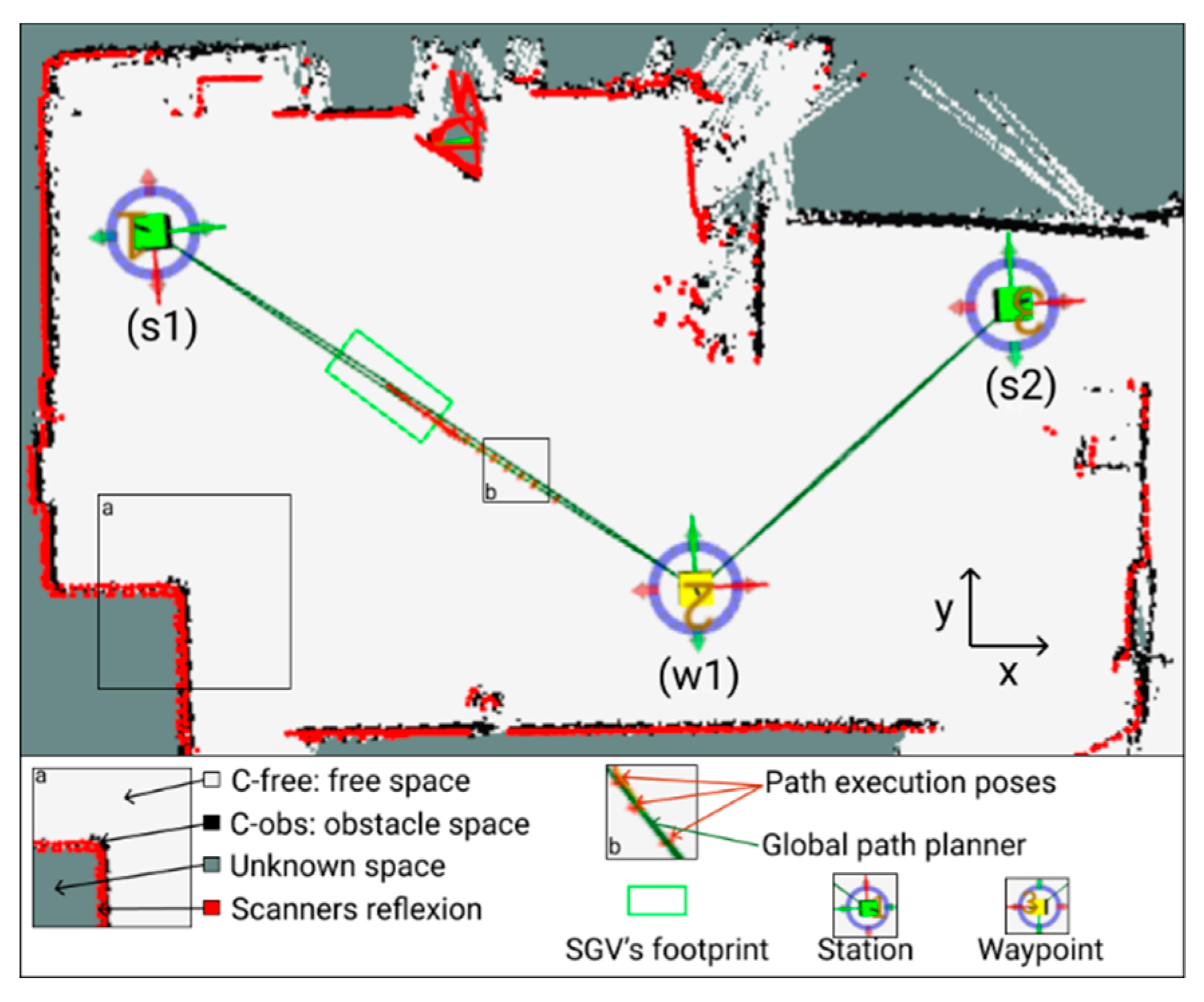
5.1. Experimental Setup

The objective of the experiment is to analyze the link between the energy level of a typical industrial SGV (see characteristics in Table 2) and its operational performance in real environment. Essential to the smooth and safe execution of the mission, the navigation performance of the autonomous platform is likely to be affected by the low battery level.
A differential-drive platform generally consists of a rigid body (base or chassis) with two motorized wheels with a common axis of rotation and four swivel wheels at the corners, with a smaller diameter, whose function is to keep the robot statically balanced (see Figure 10 and Figure 11). The Instantaneous Center of Rotation (ICR) is a point about which the nonholonomic platform rotates.
Equations (1)–(4) show that by varying the velocities of the two wheels, the ICR moves along the axle by a distance R from the center, thus, the trajectory (see Figure 11).
( V r , V l ) = ( ω ( R + L 2 ) ,   ω ( R L 2 ) )
R = L 2 V r + V l V r V l
ω = V r V l L
ICR = ( ICRx ICRy ) = ( x Rsin ( θ )   y + Rcos ( θ ) ) .  
where, L is the distance between the centers of the two wheels, Vr, Vl are the right and the left wheel translational velocities along the ground reference, ω is the rotation velocity of the vehicle body, and R is the distance from ICR to the midpoint between the wheels.
For this type of configuration, the forward kinematics of the differential-drive at time t = t + δ t is described by the following equations [59,60]:
[ x y θ ] = [ cos ( ω δ t ) sin ( ω δ t ) 0 sin ( ω δ t ) cos ( ω δ t ) 0 0 0 1 ] + [ x ICRx y ICRy θ ] + [ ICRx ICRy ω δ t ]
The SGV’s differential drive configuration are convenient for an obstacle-cluttered environment, due to the fact that the ICR can be close to the center of mass. The flexibility and agility of these vehicles allow them to be used for freight applications in an industrial environment.

5.2. Scenario

We propose a dynamic obstacle free scenario that consists of translational and rotation motions. The SGV has to carry a load of 40 kg for several laps, from station s1 to station s2, then go back to s1 (see Figure 12), every time passing through waypoint w1. The maximum translational and angular velocities of motion execution are respectively: Vmax = 0.8 m/s and Ωmax = 0.5 rad/s.
The global planner A* is used to generate the reference trajectory that must be followed by the SGV. Each reference vehicle pose q is defined as followed:
q R = [ x R y R θ R ]
where ( x R , y R ) is the coordinate of the SVG center of gravity in the reference frame as shown in Figure 12. θ R is the planned SVG orientation. As the vehicle is moving, each pose qk at the timestamp k, is represented by:
q k = [ x k y k θ k ]
where at timestamp k, ( x k , y k ) is the coordinate of the SVG center of gravity in the reference frame as provided by the onboard localization module. θ R is the SVG orientation as given by the localization module.
For each lap, a mean square error (MSE) is computed based on Equation (3). This indicator has been selected because of its wide acceptance a good performance metric when comparing two time-series [61].
MSE = 1 n k = 1 n ( ( x C x k ) 2 + ( y C y k ) 2 )
where n is the number of poses between the start and the end poses for a specific lap. xc and yc represent coordinate of the closest reference pose to qk, respectively.
Based on the above mentioned definition, any value of MSE close to 0 is an indication of a perfect reference trajectory following. Conversely, when the MSE value is increasing, the SVG is deviating from the prescribed reference trajectory. The battery state-of-charge is competed after each lap l as followed:
SOC l = SOC l - 1 k = 1 n I k Δ T C bat
where SOC l - 1 is the estimated battery SOC after executing the lap (l-1), I k is the measured current provided by the battery at the timestamp k, Δ T is sampling delta time, Cbat is the battery nominal capacity.

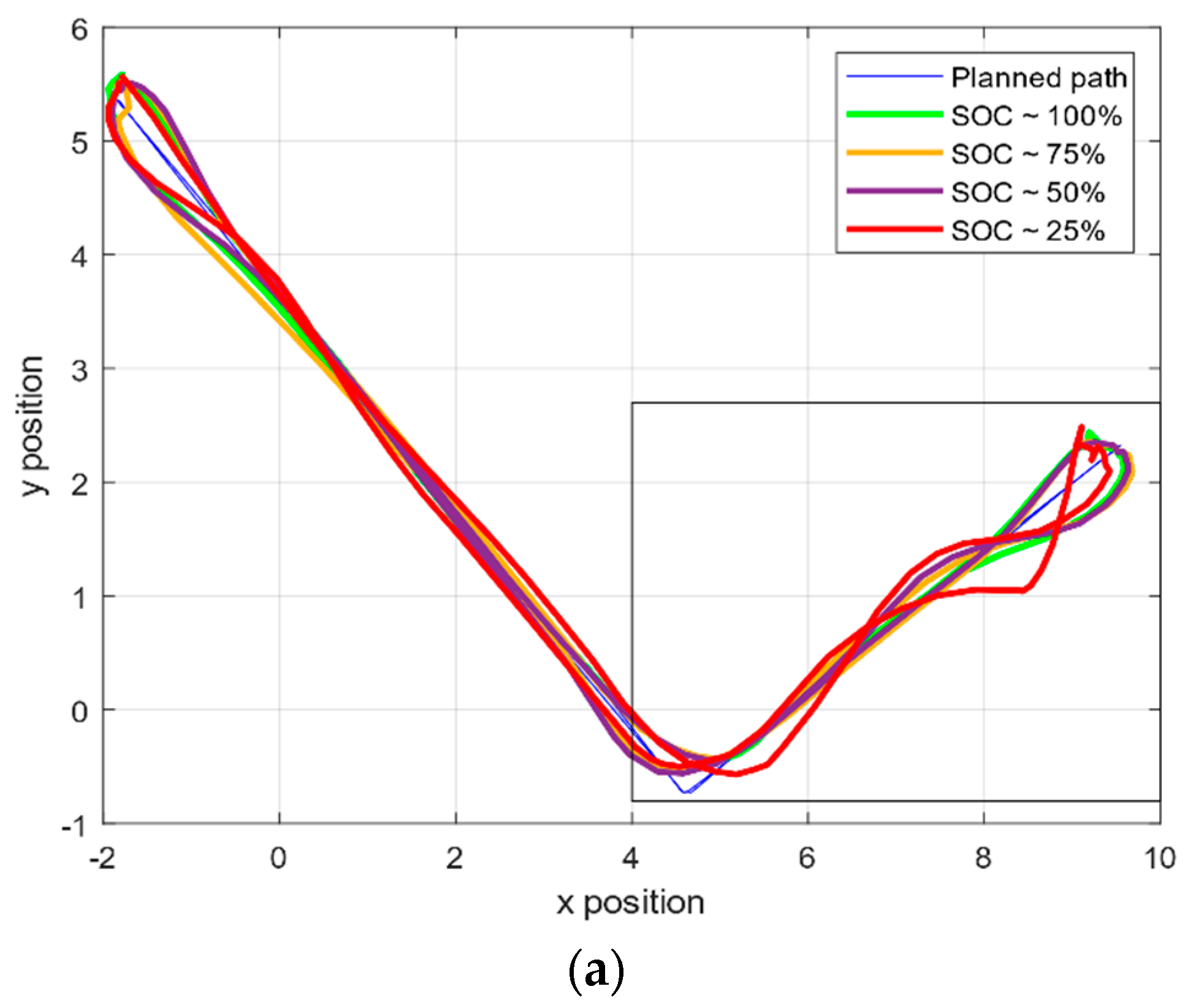
5.3. Results & Discussions

The battery is initially fully charged and we assumed that at the beginning of the first lap the SOC 1   =   100 % . A total of 600 laps that took more than 8 h have been executed by the industrial SVG. Five trajectories are represented in Figure 13. The thin blue line represents the reference trajectory while the green, yellow, purple, and red represent the trajectories executed at 100, 75, 50, and 25% SOC, respectively.
We observed, according to Figure 14 that for a SOC higher than 50%, the MSE does not exceed 0.015 ( l     520 ). Hence, the movement of the platform is close to the reference trajectory (represented on the green surface in Figure 14). When the SOC is between 25% and 50%, the SGV loses precision (orange surface), mainly when performing turns. Below 25% SOC, the MSE becomes significantly high (red surface). For several times, the SGV swerves around the global planner (see red trajectory in Figure 13b); this could be dangerous for the neighboring obstacles. Moreover, we observed that the trajectory is unsmooth at turns; this is due to the current spikes that causes the platform to jerk.
The surface A, B, and C of Figure 14 represent the evaluation indicator for the navigation performance. In surface A, the MSE indicates that the SGV performances are regular. In portion B of the curve, the gap error has increased, therefore, the planned trajectory has to be constrained in order to not reach the critical navigation represented in C. We have observed that execution time per one lap is slightly increasing when the error increases. We also noted that the high deviations occur when making rotation. These observations result in the fact that the trajectory with high dynamic efforts, mainly rotations, affects the sensing for localization due to current peaks. The observed phenomena shows the importance of monitoring the performance of SGV in real-time in order to adapt the trajectory with respect to the available battery level.
The velocity profiles of the SGV varies for different battery levels. The translational velocity variation for a lap at around 25% SOC is shown in Figure 15; the velocity signals undergoes a chattering effect compared to the velocity at 50%, which is smoother. In addition, the angular velocity profile (see Figure 16) indicates that for a lower battery level, angular speed variation is less smooth, where values reach higher peak values.
To illustrate the importance of adapting the vehicle motion, a simulation is carried out on ROS with a vehicle model integrated in a Gazebo environment. The energy model validated in [62] has four main terms represented by Equations (10)–(14). The total energy consumed by the mobile platform is ESGV.
E SGV =   E DC +   E F +   E K +   E E
where EDC, is the energy consumed by the direct current motors defined as:
E DC =   ( ( I a r ) 2 R a r +   ( I a l ) 2 R a r ) dt
where I a r and I a l are the armature currents, and R a r and R a l are the armature resistance of the left and right DC motors respectively.
The energy dissipated through friction is represented by EF:
E F =   μ mg ( ( V r ( t ) Lw r ( t ) ) + ( V l ( t ) Lw l ( t ) ) ) dt
where μ is the coefficient of rolling friction, m is the robot mass, g is the gravity, Vr and wr are the linear and angular velocities of the right wheel, Vl and wl are the linear and angular velocities of the left wheel, and L is the axle length of the vehicle.
The kinetic energy EK is due to motion and is expressed as:
E K =   1 2   ( mV 2 + I ω 2 )
V = V r + V l 2
where V and ω (defined in Equation (3)) are the linear and angular velocities of the vehicle, m is the mass, and I is the moment of inertia of the vehicle.
The energy consumed by the embedded circuitry is represented by EE, is given by the following equation:
E E =   ( I elec V elec ) dt
where I elec and V elec are, respectively, the flowing current at the battery and and the supply voltage.
Equations (10)–(15) show that the main terms that affect the total energy are the two velocities. In order to measure the effect of these velocities and battery level on the total energy, we have defined three main case studies with the same scenario, as in Figure 12. Then, the translational and rotational velocities are decreased by 5%, for 25% SOC. Then, based on the energy model, the total energy consumed for a single lap is measured, then compared to the one spent at the initial velocities (see Table 3).
The execution times shown in Table 3 are comparable to the analysis presented in [58], where the authors have depicted the minimum time required for identical autonomous mobile platforms to travel a certain distance. It has been stated that the vehicle with the lowest initial battery level executes the planned trajectory slower than the other ones, in order to reach its destination. Nevertheless, the reason is not clearly provided. In our experiment, we have quantified the difference between the three cases. In CS 2, it is observed that 4% more energy is spent compared to CS1, in order to complete a single lap. This is due to the time and effort required to self-correct the error between the path execution and the global reference path (represented in Figure 13 and Figure 14). Therefore, more energy is spent due to rotational movement as shown in the two profiles of Figure 16. The rotational movements tend to increase in an environment with several SGVs or other dynamic subjects such as human workers. So, the overall SGV-system is expected to be more energy consuming when operating in such environments.
Furthermore, in CS3, we have been capable to demonstrate that forcing the navigation system to limit its velocities by 5% from the maximum values, would save up to 3% of the total amount of energy needed to complete a lap, when the SOC drops to 25%. Therefore, regarding the limited performance of the battery-powered SGV, it is important to adapt the trajectory, by an up-front consideration of the available resources. In fleet deployment scenarios, the SGV-system efficiency will depend essentially on how the trajectories respective to each SGV are generated. In addition, the lack of resource consideration may generate ineffective trajectories that may compromise the operations before completion.
Performance measure of SGVs have mainly evolved towards safety of working environment. However, performance analysis regarding navigation and sustainability have begun only recently. With this in mind, the prism of the review and the investigation is to open a research breach regarding the sustainability of SGV-systems. We performed a simple navigation experiment with an industrial SGV, and the results show that the platform deviates from the planned path as the battery level depletes. When the battery level drops below 25% SOC, the SGV pose deviates up to 2 m from the planned position. This might jeopardise the nearby workers or platforms.
As mentioned previously, the conducted experiment did not consider the uncertainties related to localization algorithms that might negatively affect the planning and the execution of trajectories. In addition, considering the battery dynamic model allows an adequate representation of the battery’s real discharge rate. Nevertheless, these results contribute to an understanding of the navigation performances regarding the battery level, which are often neglected. Moreover, this would help industrials to evaluate the operational sustainability of their fleet capabilities.

6. Conclusions

To reach higher performances, the Industry 4.0 paradigms tend to be holistic, and pose several challenges, mainly for efficient navigation scenarios. This manuscript introduces an aspect of resource-based sustainability related to the multivehicle-based system. Systematic consideration of resources in path planning design, is as far as we know, not extensively covered in literature. Moreover, a negative impact on the navigation performances are observed. The conducted experiment has provided two main aspects. First, the MSE between the planned path and the ground-true poses, when the SOC is below 30%, may reach 5 times the value at condition where the SOC is above 30%. This is mainly due to the lack of consistency of decision-action taken by the SGV’s navigation system. Second, the mobile platform spends up to 4% more energy, and taking longer to reach its destination with around 3% more time to self-correct its own poses with respect to the planned path. These differences would be higher when traveling further distances.
This paper provides the initial foundation for further research, and allows us to reach conclusion on how essential an effective energy resource management is to the navigation system performance. Finding a compromise between energy and time by adapting the global trajectory based on the available resources, would lead to a more robust and energy-efficient execution, and by consequence, enhancing the overall SGV-system sustainability.
In order to extend the scope of this paper in view of future contributions, the following two points are proposed to anticipate the challenges that Industry 4.0 sustainability is bringing:
  • Considering that when allocating tasks to the SGV, the vehicle has to seek for paths, evaluate a multi-objective cost function and, based on the resource state, report in real-time whether it is able to execute the task or not.
  • Adapting the generated global trajectories based on the link between the fleet of SGVs and resource management.

Author Contributions

M.G. conceptualized the research and wrote the paper; methodology design, S.K., M.G.; software, L.Z.; optimization L.Z. and M.G.; project management, A.A.; supervision, S.K. and K.A.; M.G., L.Z., A.A. and M.M. contributed to the implementation of the mobile platform. All authors have read and agreed to the published version of the manuscript.

Funding

This research received no external funding.

Acknowledgments

The authors would like to thank Noovelia Inc., Fondation de l’Université du Québec à Trois-Rivières and the Canada Natural Science and Engineering Research Council for their support.

Conflicts of Interest

The authors declare no conflict of interest.

References

  1. Flämig, H. Autonomous vehicles and autonomous driving in freight transport. In Autonomous Driving; Springer: Berlin, Germany, 2016; pp. 365–385. [Google Scholar]
  2. Li, P.; Liu, X. Common Sensors in Industrial Robots: A Review; Journal of Physics: Conference Series; IOP Publishing: Bristol, UK, 2019. [Google Scholar]
  3. Devy, M.; Chatila, R.; Fillatreau, P.; Lacroix, S.; Nashashibi, F. On autonomous navigation in a natural environment. Robot. Auton. Syst. 1995, 16, 5–16. [Google Scholar] [CrossRef]
  4. Zhong, R.Y.; Xu, X.; Klotz, E.; Newman, S. Intelligent manufacturing in the context of industry 4.0: A review. Engineering 2017, 3, 616–630. [Google Scholar] [CrossRef]
  5. Efthymiou, O.Κ.; Ponis, S.T. Current Status of Industry 4.0 in Material Handling Automation and In-house Logistics. Int. J. Ind. Manuf. Eng. 2019, 13, 1370–1374. [Google Scholar]
  6. Apostolos, F.; Alexios, P.; Georgios, P.; Panagiotis, S.; George, C. Energy efficiency of manufacturing processes: A critical review. Procedia CIRP 2013, 7, 628–633. [Google Scholar] [CrossRef] [Green Version]
  7. Bonilla, S.H.; Silva, H.R.O.; da Silva, M.T.; Gonçalves, R.F.; Sacomano, J.B. Industry 4.0 and sustainability implications: A scenario-based analysis of the impacts and challenges. Sustainability 2018, 10, 3740. [Google Scholar] [CrossRef] [Green Version]
  8. Shrouf, F.; Ordieres, J.; Miragliotta, G. Smart factories in Industry 4.0: A review of the concept and of energy management approached in production based on the Internet of Things paradigm. In Proceedings of the 2014 IEEE International Conference on Industrial Engineering and Engineering Management, Bandar Sunway, Malaysia, 9–12 December 2014. [Google Scholar]
  9. Ahmed, E.; Yaqoob, I.; Gani, A.; Imran, M.; Guizani, M. Internet-of-things-based smart environments: State of the art, taxonomy, and open research challenges. IEEE Wirel. Commun. 2016, 23, 10–16. [Google Scholar] [CrossRef]
  10. Beier, G.; Niehoff, S.; Xue, B. More sustainability in industry through industrial internet of things? Appl. Sci. 2018, 8, 219. [Google Scholar] [CrossRef]
  11. Wu, S.; Wu, Y.; Chi, C. Development and application analysis of AGVS in modern logistics. Rev. Fac. Ing. 2015, 32, 380–386. [Google Scholar]
  12. Gaur, A.; Pawar, M. AGV Based Material Handling System: A Literature Review. Int. J. Res. Sci. Innov. 2016, Volume III. [Google Scholar]
  13. Naiqi, W.; MengChu, Z. Modeling and deadlock avoidance of automated manufacturing systems with multiple automated guided vehicles. IEEE Trans. Syst. Man Cybern. Part B (Cybern.) 2005, 35, 1193–1202. [Google Scholar]
  14. Draganjac, I.; Miklic, D.; Kovacic, Z.; Vasiljevic, G.; Bogdan, S. Decentralized Control of Multi-AGV Systems in Autonomous Warehousing Applications. IEEE Trans. Autom. Sci. Eng. 2016, 13, 1433–1447. [Google Scholar] [CrossRef]
  15. De Ryck, M.; Versteyhe, M.; Debrouwere, F. Automated guided vehicle systems, state-of-the-art control algorithms and techniques. J. Manuf. Syst. 2020, 54, 152–173. [Google Scholar] [CrossRef]
  16. Raja, P.; Pugazhenthi, S. Optimal path planning of mobile robots: A review. Int. J. Phys. Sci. 2012, 7, 1314–1320. [Google Scholar] [CrossRef]
  17. Hachour, O. Path planning of Autonomous Mobile robot. Int. J. Syst. Appl. Eng. Dev. 2008, 2, 178–190. [Google Scholar]
  18. Bechtsis, D.; Tsolakis, N.; Vlachos, D.; Iakovou, E. Sustainable supply chain management in the digitalisation era: The impact of Automated Guided Vehicles. J. Clean. Prod. 2017, 142, 3970–3984. [Google Scholar] [CrossRef] [Green Version]
  19. Valero, F.; Rubio, F.; Llopis-Albert, C. Assessment of the Effect of Energy Consumption on Trajectory Improvement for a Car-like Robot. Robotica 2019, 37, 1998–2009. [Google Scholar] [CrossRef]
  20. Fedorenko, R.; Gurenko, B. Local and Global Motion Planning for Unmanned Surface Vehicle. In MATEC Web of Conferences; EDP Sciences: Les Ulis, France, 2016. [Google Scholar]
  21. Anavatti, S.G.; Francis, S.L.; Garratt, M. Path-planning modules for autonomous vehicles: Current status and challenges. In Proceedings of the 2015 International Conference on Advanced Mechatronics, Intelligent Manufacture, and Industrial Automation (ICAMIMIA), Surabaya, Indonesia, 15–17 October 2015. [Google Scholar]
  22. Lozano-Pérez, T.; Wesley, M.A. An algorithm for planning collision-free paths among polyhedral obstacles. Commun. ACM 1979, 22, 560–570. [Google Scholar] [CrossRef]
  23. Patle, B.; Babu, G.; Pandey, A.; Parhi, D.; Jagadeesh, A. A review: On path planning strategies for navigation of mobile robot. Def. Technol. 2019, 15, 582–606. [Google Scholar] [CrossRef]
  24. Yu, K. Finding a natural-looking path by using generalized visibility graphs. In Pacific Rim International Conference on Artificial Intelligence; Springer: Berlin, Germany, 2006. [Google Scholar]
  25. Ó’Dúnlaing, C.; Yap, C.K. A “retraction” method for planning the motion of a disc. J. Algorithms 1985, 6, 104–111. [Google Scholar] [CrossRef]
  26. Lozano-Perez, T. Robot programming. Proc. IEEE 1983, 71, 821–841. [Google Scholar] [CrossRef]
  27. Abbadi, A.; Přenosil, V. Safe path planning using cell decomposition approximation. Distance Learn. Simul. Commun. 2015, 8, 2–3. [Google Scholar]
  28. Ou, L.; Liu, W.; Yan, X.; Chen, Y.; Liang, J. A Review of Representation, Model, Algorithm and Constraints for Mobile Robot Path Planning. In Proceedings of the 2018 IEEE 4th Information Technology and Mechatronics Engineering Conference (ITOEC), Chongqing, China, 14–16 December 2018. [Google Scholar]
  29. Huang, H.; Tsai, C. Global path planning for autonomous robot navigation using hybrid metaheuristic GA-PSO algorithm. In Proceedings of the SICE Annual Conference 2011, Tokyo, Japan, 13–18 September 2011. [Google Scholar]
  30. Huang, H.-C. FPGA-based hybrid GA-PSO algorithm and its application to global path planning for mobile robots. Prz. Elektrotech. 2012, 88, 281–284. [Google Scholar]
  31. Châari, I.; Koubaa, A.; Bennaceur, H.; Trigui, S.; Al-Shalfan, K. SmartPATH: A hybrid ACO-GA algorithm for robot path planning. In Proceedings of the 2012 IEEE Congress on Evolutionary Computation, Brisbane, Australia, 10–15 June 2012. [Google Scholar]
  32. Masehian, E.; Sedighizadeh, D. Classic and heuristic approaches in robot motion planning-a chronological review. World Acad. Sci. Eng. Technol. 2007, 23, 101–106. [Google Scholar]
  33. Takahashi, K.; Tomah, S. Online optimization of AGV transport systems using deep reinforcement learning. Bull. Netw. Comput. Syst. Softw. 2020, 9, 53–57. [Google Scholar]
  34. Xue, T.; Zeng, P.; Yu, H. A reinforcement learning method for multi-AGV scheduling in manufacturing. In Proceedings of the 2018 IEEE International Conference on Industrial Technology (ICIT), Lyon, France, 20–22 February 2018. [Google Scholar]
  35. Kamoshida, R.; Kazama, Y. Acquisition of Automated Guided Vehicle Route Planning Policy Using Deep Reinforcement Learning. In Proceedings of the 2017 6th IEEE International Conference on Advanced Logistics and Transport (ICALT), Bali, Indonesia, 24–27 July 2017. [Google Scholar]
  36. Otte, M.W. A Survey of Machine Learning Approaches to Robotic Path-Planning; University of Colorado at Boulder: Boulder, CO, USA, 2015. [Google Scholar]
  37. Fusic, J.; Kanagaraj, G.; Hariharan, K. Autonomous Vehicle in Industrial Logistics Application: Case Study. In Industry 4.0 and Hyper-Customized Smart Manufacturing Supply Chains; IGI Global: Hershey, PA, USA, 2019; pp. 182–208. [Google Scholar]
  38. Llopis-Albert, C.; Rubio, F.; Valero, F. Optimization approaches for robot trajectory planning. Multidiscip. J. Educ. Soc. Technol. Sci. 2018, 5, 1–16. [Google Scholar] [CrossRef] [Green Version]
  39. Abbadi, A.; Matousek, R.; Osmera, P.; Knispel, L. Spatial guidance to RRT planner using cell-decomposition algorithm. In Proceedings of the 20th International Conference on Soft Computing, MENDEL, Brno, Czech Republic, 20–22 June 2014. [Google Scholar]
  40. Noreen, I.; Khan, A.; Habib, Z. Optimal path planning using RRT* based approaches: A survey and future directions. Int. J. Adv. Comput. Sci. Appl. 2016, 7, 97–107. [Google Scholar] [CrossRef] [Green Version]
  41. Sucan, I.A.; Moll, M.; Kavraki, L.E. The Open Motion Planning Library. IEEE Robot. Autom. Mag. 2012, 19, 72–82. [Google Scholar] [CrossRef] [Green Version]
  42. Petereit, J. Adaptive State× Time Lattices: A Contribution to Mobile Robot Motion Planning in Unstructured Dynamic Environments; KIT Scientific Publishing: Karlsruhe, Germany, 2017; Volume 27. [Google Scholar]
  43. Likhachev, M. Search-based Planning with Motion Primitives; Tutorial at CoTeSys-ROS Fall School on Cognition-enabled Mobile Manipulation; Carnegie Mellon University: Pittsburgh, PA, USA, 2010. [Google Scholar]
  44. Ravankar, A.; Ravankar, A.A.; Kobayashi, Y.; Hoshino, Y.; Peng, C.-C. Path smoothing techniques in robot navigation: State-of-the-art, current and future challenges. Sensors 2018, 18, 3170. [Google Scholar] [CrossRef] [Green Version]
  45. Ferguson, D.; Likhachev, M.; Stentz, A. A guide to heuristic-based path planning. In Proceedings of the International Workshop on Planning under Uncertainty for Autonomous Systems, International Conference on Automated Planning and Scheduling (ICAPS), Berkeley, CA, USA, 5–10 June 2005. [Google Scholar]
  46. Stentz, A. The Focussed D* Algorithm for Real-Time Replanning. In Proceedings of the International Joint Conference on Artificial Intelligence, Montréal, QC, Canada, 20–25 August 2020. [Google Scholar]
  47. Hada, Y.; Yuta, S. Robust navigation and battery re-charging system for long term activity of autonomous mobile robot. In Proceedings of the 9th International Conference on Advanced Robotics, Tokyo, Japan, 25–27 October 1999. [Google Scholar]
  48. Oh, S.; Zelinsky, A.; Taylor, K. Autonomous battery recharging for indoor mobile robots. In Proceedings of the Australian Conference on Robotics and Automation, Brisbane, Australia, 2–4 October 2000. [Google Scholar]
  49. Silverman, M.C.; Nies, D.; Jung, B.; Sukhatme, G.S. Staying alive: A docking station for autonomous robot recharging. In Proceedings of the 2002 IEEE International Conference on Robotics and Automation, Washington, DC, USA, 11–15 May 2002. Cat. No. 02CH37292. [Google Scholar]
  50. Wang, T.; Wang, B.; Wei, H.; Cao, Y.; Wang, M.; Shao, Z. Staying-alive and energy-efficient path planning for mobile robots. In Proceedings of the 2008 American Control Conference, Seattle, WA, USA, 11–13 June 2008. [Google Scholar]
  51. Strimel, G.P.; Veloso, M.M. Coverage planning with finite resources. In Proceedings of the 2014 IEEE/RSJ International Conference on Intelligent Robots and Systems, Chicago, IL, USA, 14–18 September 2014. [Google Scholar]
  52. Hussein, A.M.; Elnagar, A. On smooth and safe trajectory planning in 2d environments. In Proceedings of the International Conference on Robotics and Automation, Albuquerque, NM, USA, 25 April 1997. [Google Scholar]
  53. Chaudhari, M.; Vachhani, L.; Banerjee, R. Towards optimal computation of energy optimal trajectory for mobile robots. IFAC Proc. Vol. 2014, 47, 82–87. [Google Scholar] [CrossRef]
  54. Liu, S.; Sun, D. Minimizing energy consumption of wheeled mobile robots via optimal motion planning. IEEE/ASME Trans. Mechatron. 2013, 19, 401–411. [Google Scholar] [CrossRef]
  55. Tokekar, P.; Karnad, N.; Isler, V. Energy-optimal trajectory planning for car-like robots. Auton. Robot. 2014, 37, 279–300. [Google Scholar] [CrossRef]
  56. Kelouwani, S.; Agbossou, K.; Dubé, Y.; Boulon, L. Energetic optimization of the driving speed based on geographic information system data. In Proceedings of the 2012 IEEE Vehicular Technology Conference (VTC Fall), Quebec City, QC, Canada, 3–6 September 2012. [Google Scholar]
  57. Mejri, E.; Kelouwani, S.; Dube, Y.; Trigui, O.; Agbossou, K. Energy efficient path planning for low speed autonomous electric vehicle. In Proceedings of the 2017 IEEE Vehicle Power and Propulsion Conference (VPPC), Belfort, France, 11–14 December 2017. [Google Scholar]
  58. Setter, T.; Egerstedt, M. Energy-constrained coordination of multi-robot teams. IEEE Trans. Control Syst. Technol. 2016, 25, 1257–1263. [Google Scholar] [CrossRef]
  59. Siciliano, B.; Villani, L.; Oriolo, G.; Sciavicco, L. Robotics: Modelling, Planning and Control; Springer Science & Business Media: New York, NY, USA, 2010. [Google Scholar]
  60. Dudek, G.; Jenkin, M. Computational Principles of Mobile Robotics; Cambridge University Press: Cambridge, UK, 2010. [Google Scholar]
  61. Bostelman, R.; Hong, T.; Cheok, G. Navigation performance evaluation for automatic guided vehicles. In Proceedings of the 2015 IEEE International Conference on Technologies for Practical Robot Applications (TePRA), Woburn, MA, USA, 11–12 May 2015. [Google Scholar]
  62. Ghobadpour, A.; Amamou, A.; Kelouwani, S.; Zioui, N.; Zeghmi, L. Impact of Powertrain Components Size and Degradation Level on the Energy Management of a Hybrid Industrial Self-Guided Vehicle. Energies 2020, 13, 5041. [Google Scholar] [CrossRef]
Figure 1. Article’s research interest.
Sustainability 12 08541 g001
Figure 2. Factors influencing design and operation of Material Handling System [12].
Sustainability 12 08541 g002
Figure 3. Navigation phases of a mobile platform [17].
Sustainability 12 08541 g003
Figure 4. Navigation Stack in industry 4.0 [20].
Sustainability 12 08541 g004
Figure 5. This figure illustrates the Road-Map representation: (a) Visibility graph. (b) Voronoi diagram [23].
Sustainability 12 08541 g005
Figure 6. (a) Grid cell decomposition. (b) Adaptive cell decomposition. (c) Exact cell decomposition [27].
Sustainability 12 08541 g006
Figure 7. Machine-learning for SGV-system [37].
Sustainability 12 08541 g007
Figure 8. (a) Separate planning at waypoint wp, (b) Combined planning trough wp.
Sustainability 12 08541 g008
Figure 9. Efficient offline global trajectory planning.
Sustainability 12 08541 g009
Figure 10. A differential-drive Self-Guided Vehicle.
Sustainability 12 08541 g010
Figure 11. Kinematics of a differential-drive configuration. The red bold arrow refers to the heading of the vehicle.
Sustainability 12 08541 g011
Figure 12. The pixel map representing the free space in white and obstacles in black. The red pixels refer to the laser scanners sight.
Sustainability 12 08541 g012
Figure 13. Executed trajectory for laps at different state-of-charge levels. (b) is the zoom of the rectangle in (a).
Sustainability 12 08541 g013aSustainability 12 08541 g013b
Figure 14. The mean square error (MSE) and state-of-charge (SOC) variation for the last 100 laps.
Sustainability 12 08541 g014
Figure 15. Translational velocity profiles completing a lap at 50% and 25% SOC.
Sustainability 12 08541 g015
Figure 16. Angular velocity profiles for a single lap at around 50% and 25% SOC.
Sustainability 12 08541 g016
Table 1. Comparison between Automated Guided Vehicles (AGV)-system and Self-Guided Vehicles (SGV)-system control architectures.
SystemAGV-SystemSGV-System
System ArchitectureCentralizedDecentralized
Global optimalitySuboptimality
Simplistic guidelinesComplex navigation system
Small scaled systemLarge scaled system
Central communicationIntervehicle communication
Map representationTopological-map: A series of a point route connecting different locations,
no dynamic obstacles representation.
Pixel-map: a high-resolution occupancy grid. It uses configuration space for static obstacles representation in the environment, dynamic obstacles represented.
LocalizationBasic physical localization sensors.Advanced localization algorithms with sensor fusion of GPS, laser scan, vision-based.
Trajectory PlanningUses: direct search algorithm, on a fixed flow path layout.
Less flexible paths.
Uses: sample-based algorithm, search-based algorithms, graph search algorithm,
replanning in case of deadlocks,
constrained path such as time, energy, and distance.
Motion ExecutionNot robust to dynamics. Line following motion.Robust in dynamic situation with motion algorithms such, obstacle avoidance.
SustainabilityLess flexible to energy issues.Flexible for solving resource management issues
Table 2. The platform characteristics.
ParameterValue
Maximum Speed1.5 m/s (5 Km/h)
Vehicle Weight90 Kg
Maximum Load Carrying120 Kg
Battery Lifetime 17 h to 9 h
Dimensions (length × width × height)165 × 76 × 23 cm
1 Continuous operation at maximum load.
Table 3. Comparative data for a single lap execution at critical SOC.
Case StudyMaximum VelocitiesBattery SOCTotal Energy ESGV
(Joule)
Execution Time
(Second)
Difference in Percentage
Vmax (m/s) ω max (rad/s)EnergyTime
CS10.800.5SOC = 50%806451.3--
CS20.800.5SOC = 25%8388 52.5 +4.0%+2.3%
CS30.760.47SOC = 25%8132 53.6 +0.8%+4.5%
Publisher’s Note: MDPI stays neutral with regard to jurisdictional claims in published maps and institutional affiliations.

