Article

The Impacts of Urban Air Pollution Emission Density on Air Pollutant Concentration Based on a Panel Model

Department of Urban Engineering, Chungbuk National University, Chungdae-ro 1, Seowon-Gu, Cheongju, Chungbuk 28644, Korea
*
Author to whom correspondence should be addressed.
Sustainability 2020, 12(20), 8401; https://doi.org/10.3390/su12208401
Submission received: 6 August 2020 / Revised: 9 September 2020 / Accepted: 28 September 2020 / Published: 13 October 2020
(This article belongs to the Section Sustainable Urban and Rural Development)

Abstract

:
In terms of urban planning, the impact of urbanization and high density on the environment is a major issue. This study intended to analyze the effect of spatial density characteristics of urban air pollution sources on urban air pollution concentration using a panel model. As the total population density, the number of cars registered per capita, and the total emission facility density increased, together with a closer distance to a thermal power plant, the nitrogen dioxide(NO2) concentration increased. Net population density was also found to have the greatest impact on the structure and density of emission sources of ozone(O3) followed by the number of cars registered per person and the total emission facility density. It was confirmed that particular matter(PM10) concentrations are strongly influenced in positive directions by the spatial density characteristics of emission sources that show significant differences between regions.

1. Introduction

Currently, more than 50 percent of the world’s population resides in urban areas and is expected to reach approximately 70 percent by 2050 [1]. Korea has experienced rapid urbanization in the process of rapid economic growth and industrialization. Air pollution is one of the undesired results of rapid urbanization and has a negative impact on various public health fields [2]. It is estimated that approximately 3.7 million people die each year due to air pollution globally [3].
The emission of air pollutants and air quality are influenced by natural factors such as climate and topography. Moreover, air pollutants are emitted from various sources such as industry and transportation and are affected by socioeconomic factors. Air pollution is also closely related to urban land use patterns [4], and the distribution and form of land use affect air quality by influencing land use and the spatial distribution of human activities [5].
Urbanization and high density are the most controversial topics [6]. Although previous studies have explained the effects of land use and urban structure on air pollution, these studies have limitations of considering only the limited aspects of land use and urban structure. Most of the studies on land use mainly analyzed the effects of land use on air pollution by using the size of each land use and the ratio of these sizes. Previous studies examining urban structures evaluated the relationship between air quality and urban sprawl/compact indices (e.g., density, street network, and complexity). In conclusion, research is needed to comprehensively evaluate the effects of various air pollution sources, which influence urban air pollution levels, based on land use and land structural characteristics.
Considering that population density and development intensity are key indicators of urban sprawl [7], it is necessary to analyze the impact of land use and urban structural characteristics on air pollution by introducing the density concept that can represent the development intensity of each air pollution source. Moreover, it has been found that the emission characteristics of air pollutants vary due to the seasonal changes in climate and weather. Empirical studies have also shown that the effects of temperature on air pollution concentration vary by air pollutants and regions [8,9,10]. These results strongly suggest that is necessary to comprehensively analyze the seasonal effects of weather and climate on each air pollutant at a regional level.
Most previous empirical studies used the ordinary least square (OLS) linear regression method and spatial statistical methods to analyze the effects of land use and urban structure characteristics on air quality or pollutant emissions [7,11]. However, this method has a limitation in processing seasonal variables. There are only a few studies that empirically analyze the spatial and temporal effects of land use and urban structure on air pollution.
This study developed the following research question based on the critical review of previous studies. Do the spatial density characteristics of air pollutants affect the concentration of each air pollutant differently?
To answer the research question, this study analyzed the effects of density characteristics of air pollution sources on air pollution concentration. This study used a panel model to comprehensively understand the temporal impact and spatial impact of air pollutants on air pollution.

2. Related Literature

Various factors including climate, topography, and economic activities affect air pollution concentrations [8,12,13]. Most air pollutants are generated from interactions between human activities (e.g., increased economic activity and urbanization), social systems, and the environment [14,15]. In particular, considering that land use and urban structures promote human activities and their interactions [16], studying the effects of these structural characteristics on air pollution is a major research interest.
Land use and urban structure affect air pollution by influencing the spatial distribution of human activities [5]. Moreover, they affect the distribution of air pollutants and urban air pollution concentrations in urban environments [13]. When complex urban spaces are classified in terms of land use and urban structure, they can be classified into urban land use areas such as residential areas, commercial areas, and industrial areas and transportation networks or traffic areas connecting these areas. They emit air pollutants directly or indirectly. For example, residential and commercial areas emit air pollutants due to human activities, while industrial areas emit air pollutants due to industrial activities. In the transportation network connecting these various urban activities, the movement of cars affects air pollution. That is, air pollution is closely related to urban land use patterns [4] and the differences in urban structure are important in air pollutant emissions. Land use and urban structure determine the distributions of pollution activities and air pollution [7,17]. Overall, various empirical studies are needed to understand the impact of land use and urban structure characteristics on air pollution.
Changes in land use and urban structure are major factors deteriorating air quality. Although previous studies have shown a meaningful relationship of air pollution with land use and urban structure, both categories of empirical studies have limitations. These previous studies only evaluated limited aspects of land use and urban structure.
When the effects of each air pollution factor on air pollution concentration are examined, the influential factors differ by air pollutant, and the directional nature is different for each air pollutant. Few studies have examined comprehensive relationships using multiple urban structural variables in terms of land use. Most studies have used area of each land use (residential, commercial, industrial, and transportation) and area ratios [8,10,13,18,19,20]. Additionally, since most of these studies were conducted in North American cities, China, and Europe, it is difficult to apply the results directly to South Korean cities.
Previous studies related to urban structure examined the relationship of air quality with urban sprawl, compact, and indicators (e.g., density, distance network, and complexity). They focused on explaining the relationship with linear pollution sources (cars, roads, and traffic volume) associated with traffic among various air pollution sources in cities [8,21,22,23,24,25]. Consequently, it is necessary to comprehensively consider the structural characteristics of the various air pollution sources affecting the air pollution concentration in urban areas.
Since the development intensity is another key indicator of urban sprawl [7], it is necessary to analyze the effect of land use and urban structural characteristics on air pollution by introducing the concept of density, which can represent development intensity by air pollution source. The World Bank [26], on the other hand, argues the following are needed to improve air pollution: relocate pollution sources, promote compact city structure, and minimize air pollutant emissions. In terms of the air pollution improvement, it is necessary to examine the effect of air pollution emission density characteristics, other than traffic, on air pollution.
The general causes of air pollutant emissions showed the emission characteristics of air pollutants generally changed due to the seasonal changes in climate and weather. Moreover, empirical studies revealed that there were differences in temperature and air pollution concentrations by air pollutant and region. There was a strong positive relationship between temperature and air pollution concentrations [27]. Cárdenas Rodríguez et al. [8] showed that NO2 and PM10 had a positive relationship with temperature, and Lee [10] reported that temperature had a positive impact on O3. A lower temperature increased the amount of air pollutants [9]. This is because lower temperatures increase emissions from winter heating sources [28,29,30]. As such, the effects of climate and weather on air pollution are influenced by changes in sources and photochemical reactions depending on air pollutants and vary by the climatic characteristics of the region. Most studies considered only temperature, a single indicator, as a meteorological characteristic. On the other hand, studies considering meteorological characteristics analyzed the influential relationship only in a local area, not an entire region [31]. Therefore, it is necessary to empirically analyze the seasonal effects of weather and climate on individual air pollutants at a national level.
Most empirical studies have analyzed the relationship between land use and urban structure and air pollutant emissions to find ways to reduce the quantity of air pollutant emissions. Most of these empirical studies used ordinary least square (OLS) linear regression to analyze whether the characteristics of land use and urban structure were related to air quality or pollutant emissions. Characteristics of the study area and the objectives of the study are needed before constructing a regression model to take into account the difference between different indices [30]. In order to examine the effects of land use and urban structure variables on regional air pollution, several studies classified types (e.g., different regions [11], urban and rural [32], and cities at different levels [7]) and analyzed each type. Lu·Liu [30] and McCarty·Kaza [32] also developed planning policies based on local conditions using spatial statistical methods such as geographic weighted regression models and spatial delay error models. In particular, Muttoo et al. [33] indicated that overcoming the limitations in handling seasonal variables was the limitation of the methodology. Further studies are needed on the spatial and seasonal impact mechanisms of land use and urban structures on air pollution concentrations. There are not enough empirical analyses regarding the spatial and temporal relationships between land use and urban structure and air pollution. Studies based on panel data and regional comparisons will provide more evidence about the relationships among land use, urban structure, and environmental quality. Moreover, they will help people understand the effects of land use and urban structures on air pollution under various spatial and temporal differences.

3. Methodology

3.1. Conceptual Framework and Hypothesis

In terms of environmental engineering, previous studies have focused on the direct causes of air pollution for direct management of causal factors and implementation of environmental policies such as fuel regulation and emission regulation. However, they did not take into account the effects of spatial emission structure on air pollution sources. Economic geography and urban planning emphasize the anthropogenic aspect of air pollution sources. In other words, identification of the emission structure of sources, which requires consideration of the characteristics of air pollutant sources. In particular, for secondary pollutants produced by reactions with precursors in a space, it is necessary to comprehensively consider the characteristics of sources and urban spatial characteristics.
The review of previous studies showed that the majority of studies focused on the effects of urban density and urban sprawl on urban air pollution. It was found that the influential relationship varied by country, region, and developmental level. The main analysis results were the effect of urban land use area on air pollution. These are quantity-oriented analysis, and the pattern was different by region and pollutant. Multi-dimensional influence analyses encompassing the characteristics, quantities, and densities of air pollution sources must be conducted. It is necessary to analyze these by comprehensively considering roads, emission facilities, and urban forms.
In the theoretical discussion on air pollution sources, we need to analyze the source characteristics of primary products and the source characteristics and land use characteristics of secondary products. In particular, it is necessary to evaluate the characteristics of sources for secondary products (O3 and PM10) and conduct influence analysis with respect to the emission structure (e.g., land use characteristics) in urban spaces influencing secondary production. Additionally, we need to select an explanatory indicator reflecting the causes of production because there are differences in the generation of secondary products. We also need to analyze the effects of a specific period (e.g., yellow dust) and the external effects of specific weather characteristics.
Yellow dust refers to a phenomenon that describes slowly descending fine sand dust, which is first blown up by wind from an arid red clay region mainly located in northern China or Mongolia, dispersed in the atmosphere, and then covers the sky or descends as a cloud of dust. It generally occurs from March to May, under low pressure, and sometimes moves to Japan, the Pacific Ocean, and North America through Korea by being carried by strong westerly winds. When a severe yellow dust phenomenon occurs, the sun appears yellowish-brown because sunlight is scattered or blocked. Moreover, sand dust often deposits on the ground.
According to the theoretical review and literature review, urban characteristics were classified into socio-economic characteristics, urban sprawl characteristics, urban density characteristics, air pollution source characteristics, and urban land use characteristics, and each influential relationship of air pollution concentrations was analyzed. This study aimed to derive comprehensive air pollution influential factors by using these variables.
Additionally, this study tried to analyze the comprehensive influential relationship affecting the concentration of each air pollutant. In particular, this study aimed to analyze the air pollution concentration relationship reflecting inter- and intra-regional differences.
Study hypotheses were established as follows based on the study conceptual model (Figure 1) to solve study questions identified by analyzing the effects of the air pollution source structure and density characteristics on air pollution concentration.
Each air pollutant has a different source, and the concentration characteristics of each pollutant vary according to the reactions in the atmosphere after being emitted. NO2 is affected by direct sources such as the fuel combustion of automobiles. Contrarily, O3 and PM10 are influenced by the external environment as well as a direct source. Furthermore, the principle of generating O3 in the atmosphere is different from that of producing PM10. We used a different set of variables for each air pollutant to analyze the spatial characteristics affecting each air pollutant. In order to evaluate the specific effects of density (among various spatial characteristics), we examined the effects of individual variables of density, rather than spatial or density characteristics.
Hypothesis 
Source density characteristics, meteorological characteristics, and yellow dust characteristics will affect the concentration of air pollutants differently.
We need to analyze the source characteristics of NO2 and the source characteristics and land use characteristics of secondary products. The source characteristics and land use characteristics of O3 and PM10 need to be analyzed. When the effects of the individual influential indicators of air pollution on air pollution concentrations were evaluated, influential factors varied by air pollutant and their directions were also different. For O3 and PM10, we need to analyze the effects of emission structures (e.g., land use characteristics) on secondary products in urban spaces as well as the characteristics of sources.
O3 concentration is greatly affected by meteorological factors such as temperature, precipitation, pollutant spread, and atmospheric stability in addition to pollutant emissions. Moreover, it is generated by photochemical reactions in the air. Therefore, countermeasures are needed. It is necessary to analyze the effects of a specific period such as yellow dust and the external effects of weather characteristics.
The monthly mean concentration pattern of PM10 has the highest level in the spring, when it is affected by yellow dust. The external effects of a specific period such as yellow dust and meteorological characteristics need to be analyzed.
Hypothesis 1 (H1).
NO2 concentrations will be affected by the total density characteristics of an air pollution source.
Hypothesis 2 (H2).
O3 will be affected by source total density, urban sprawl characteristics (population net density), sunshine, and yellow dust.
Hypothesis 3 (H3).
PM10 concentration will be affected by the density of sources and yellow dust.

3.2. Data and Methodology

3.2.1. Selecting Variables and Establishing Data

Air pollution concentrations were measured where the urban air monitoring network was established among Airkorea’s public monitoring networks. NO2, O3, and PM10 were measured, and their monthly means were used as variables.
NO2 among the primary products and O3 and PM10 among the secondary products were selected as dependent variables. SO2 and CO among the primary products and PM2.5 among the secondary products were excluded. This is because SO2 concentration has been between 0.005 and 0.006 ppm since 2002 (threshold: 0.02 ppm). CO concentration has been 0.5 ppm since 2009 (threshold: 9 ppm). As of 2016, they have been under the thresholds all the time and there is little difference between regions. PM2.5 was excluded because it was measured at different stations compared with other substances, and measurement began in 2015, limiting panel analysis.
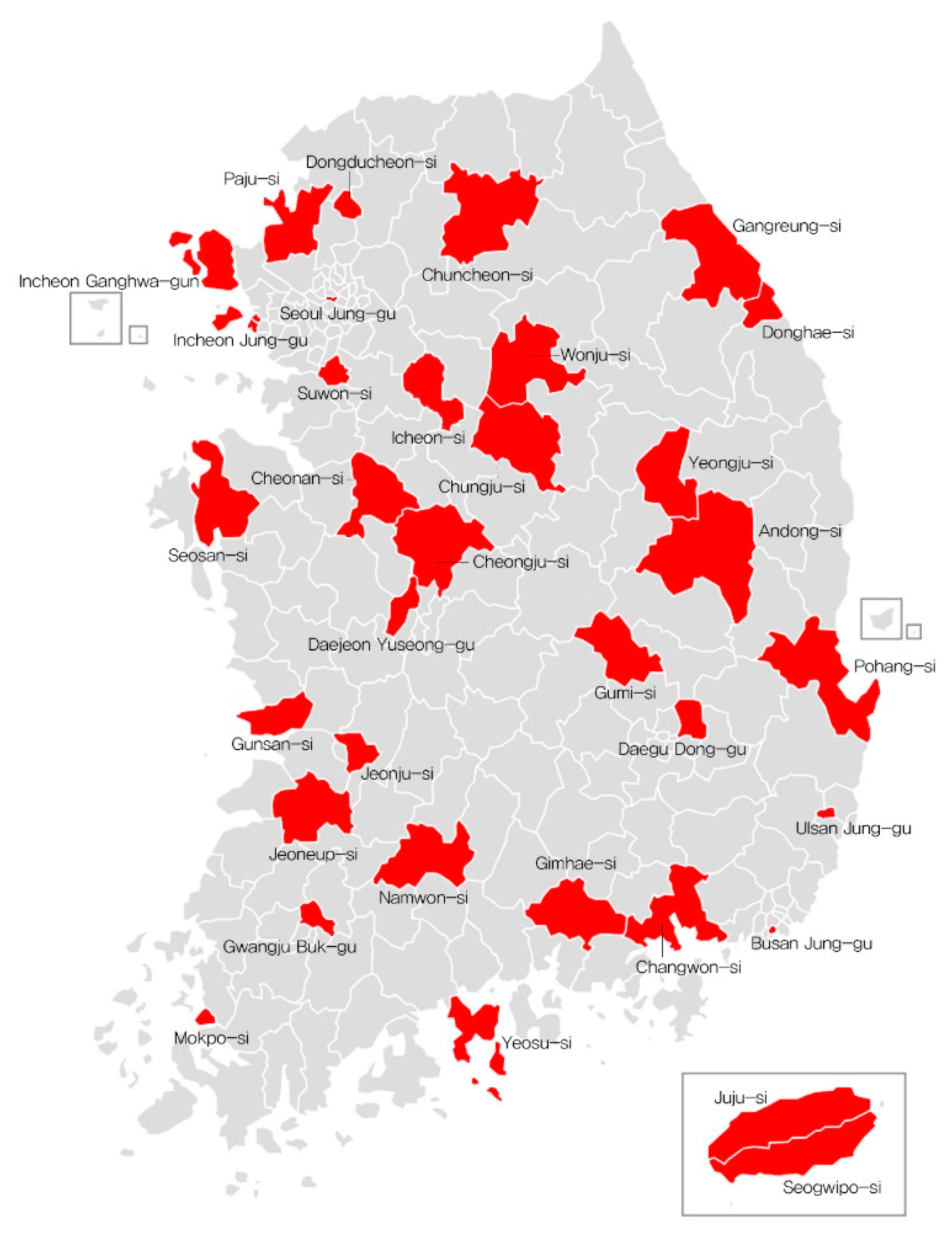
The spatial unit of analysis is 35 municipalities. Urban characteristic indicators were obtained from Statistics Korea data. Air pollution characteristics and the variable setting and explanation of urban characteristics are shown in Table 1.
The concentrations of air pollutants have a relatively short lifetime compared to the long lifetime of urban spaces. Additionally, meteorological characteristics have a different lifetime than these two. This study used a monthly time step to derive a model that combines these various characteristics. The Ministry of Environment of the Republic of Korea processes and discloses only highly reliable monthly data from data produced on an hourly basis in order to utilize the data for research and policy implementation.
The Ministry of Environment and local municipalities in Korea operate 11 types of monitoring network (urban air, roadside atmosphere, acidic precipitation, national background concentrations, suburban air, heavy metals in air, harmful air pollutants, photochemical air pollutants, atmosphere, and PM2.5). The monitoring networks are composed of 510 stations in 96 cities and counties. This study utilized the monthly measurement data measured by 11 urban air monitoring networks. The urban air monitoring network runs 264 measuring stations in 82 cities and counties as of 2016 to determine whether environmental standards have been met by identifying the mean air quality of urban areas. The networks measure SO2, CO, NOx, PM10, PM2.5, and O3 hourly. After finalizing and statistical processing of the measurement data of the nationwide measuring stations, they are stored in the form of a database. The National Institute of Environmental Research calculates statistical data only when more than 75% of the measured data are obtained during statistical processing to enhance the reliability of the statistical data. Monthly data were constructed for each municipality based on this by using the monthly air pollution level measurements from measuring stations in the finalized Air Quality Annual Report. When a municipality had more than one measuring station, the mean values of the stations in the corresponding municipality were used. Finally, air pollution measurement data were constructed for 132 municipalities.
The meteorological characteristics were determined by using the ASOS data provided by the Korea Meteorological Administration. Temperature, precipitation, wind, atmospheric pressure, humidity, solar radiation, sunshine, snow, cloud, visibility, ground condition, ground surface temperature, grass temperature, weather phenomena, and evaporation loss were measured at 95 nationwide locations. Monthly total precipitation (precipitation), mean wind speed (wind), mean temperature (temperature), mean relative humidity (humidity), and the total duration of sunshine and percentage of sunshine (sunshine and solar radiation) were utilized. When a measuring station could be included in multiple municipalities, the station mean values were calculated.
Among the 132 municipalities with available air pollution measurements, 40 municipalities (Seoul Jung-gu, Busan Jung-gu, Daegu Dong-gu, Incheon Jung-gu, Incheon Ganghwa-gun, Gwangju Buk-gu, Daejeon Yuseong-gu, Ulsan Jung-gu, Suwon-si, Dongducheon-si, Paju-si, Icheon-si, Chuncheon-si, Wonju-si, Gangreung-si, Donghae-si, Cheongju-si, Chungju-si, Jucheon-si, Cheonan-si, Seosan-si, Jeonju-si, Gunsan-si, Jeoneup-si, Namwon-si, Mokpo-si, Yeosu-si, Suncheon-si, Gwangyang-si, Pohang-si, Gyeongju-si, Andong-si, Gumi-si, Yeongju-si, Jinju-si, Gimhae-si, Yangsan-si, Changwon-si, Juju-si, Seogwipo-si) had ASOS data. Moreover, 35 municipalities, except for five municipalities (Jecheon-si, Suncheon-si, Gwangyang-si, Gyeongju-si, Yangsan-si), had strongly balanced panel data from 2008 to 2016.
We generated a map showing the geographic location of these 35 municipalities (Figure 2).

3.2.2. Study Model and Hypothesis Testing

This study established a monthly panel analysis model using the 2008 and 2016 data of 35 municipalities to analyze the effects of meteorological characteristics and air pollution source characteristics on air pollution concentrations.
This panel analysis model can estimate the effects of independent variables on dependent variables using a regression analysis that controls unobserved characteristics and unobserved heterogeneity between regions and time effects causing differences between years or months simultaneously [34].
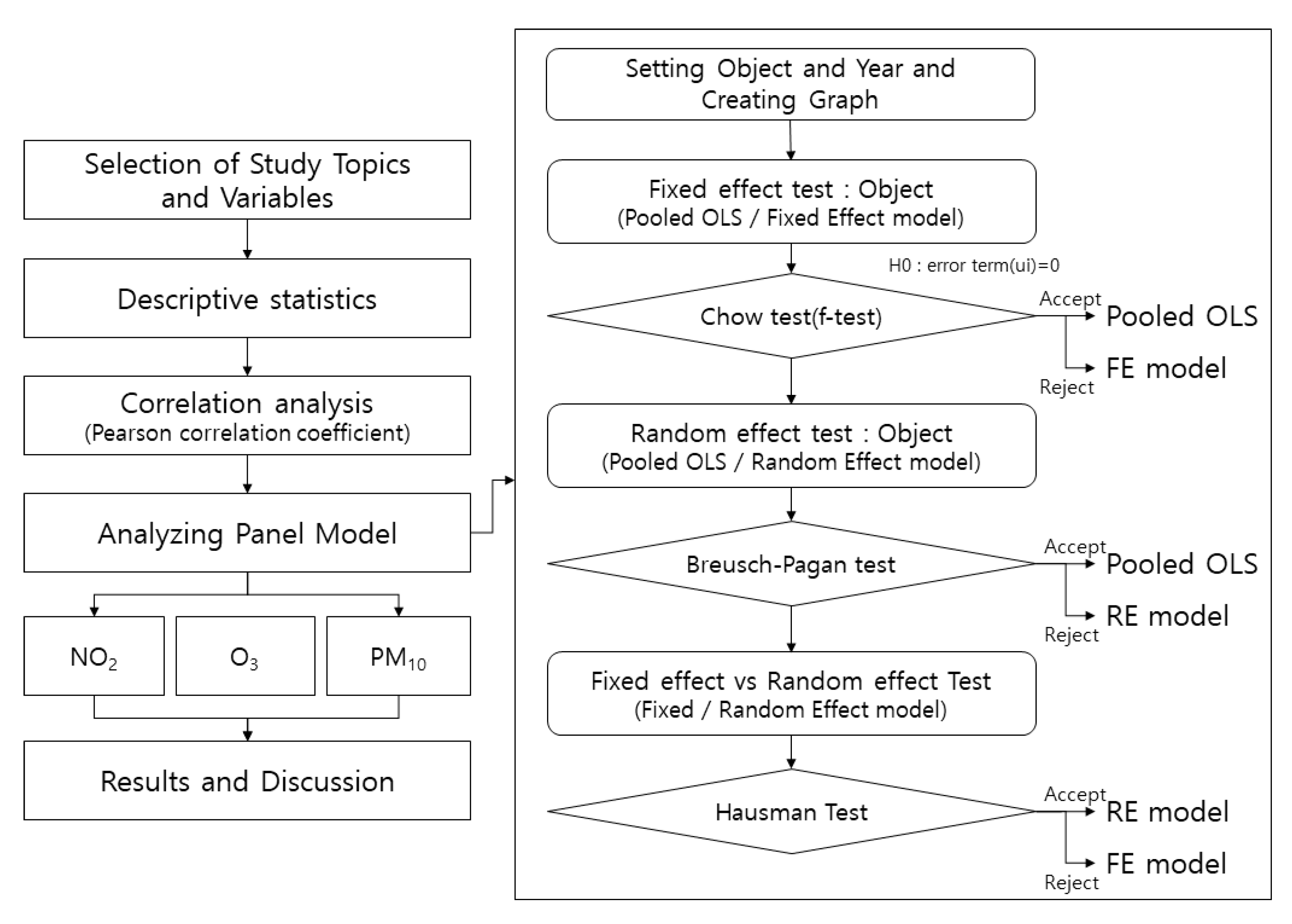
Panel analysis models can be divided into fixed effect models and random effect models. As shown in Figure 3, the validity between these two model types is determined by the Hausman test, and the final model is selected by confirming the validity using an OLS method step-by-step [35].
Based on the variables derived from the previous studies, panel data analysis was used to analyze time-series data and cross-sectional data simultaneously for estimating the effects of air pollution concentrations.
For panel model analysis, this study first set up the data structure (object and time) to be analyzed. This study established a strongly balanced panel data structure based on individuals to examine the fixed effect and random effect of municipalities.
This study examined the descriptive statistics (mean and standard deviation) of major variables that were used for this study and believed to influence the relationship between air pollutant concentrations and air pollution emission spatial density from 2008 to 2016. In addition, Pearson correlation analysis was conducted to verify the relationship between the dependent and independent variables and the correlation between the independent variables.
A pooled OLS model and a two-way error component panel model were candidate estimation models for analyzing the panel model, and the validity of individual models was tested. In the first step, a Chow test (F-test) and a Breusch–Pagan test were conducted to determine the suitability between the pooled OLS model and the two-way error component panel model. The former is required to select between the pooled OLS model and the two-way error component panel model, and the latter needs to choose between the pooled OLS model and the random effect model. To obtain consistent estimators, this study conducted the Hausman test to choose between the fixed effect model and the random effect model under the null hypothesis that (individual effects) error term (ui) and explanatory variables were not correlated (H0: cov(Xit, ui)=0).
The basic regression equation of this study has a nonlinear relationship between the explanatory variable and the dependent variable. However, it is a linear model for parameters. Therefore, the model of this study is a multiple regression linear model, and it can be estimated using the ordinary least squares (OLS) method. However, in the case of the panel data used in this study, when constant terms and individual effects (error term; ui) are stochastic variables and they are estimated using OLS, the first-order autocorrelation (AR(1)) issue may occur. Therefore, the estimation model should be tested first to resolve the first-order autocorrelation issue of the error terms and obtain efficient estimators. As a result, this study tested the validity of each model while using a pooled OLS model and a two-way error component panel model as candidate estimation models for panel data analysis.

4. Results

4.1. Descriptive Statistical Analysis

Table 2 shows the basic statistics of variables included to analyze air pollution concentration factors. Descriptive statistics (e.g., observations, mean, standard deviations, minimum, and maximum values) of the dependent and explanatory variables are presented. This study did not find a problematic variable that had too large a standard deviation or relatively small observation numbers.
When the monthly information of 35 municipalities was collected for nine years, 3780 datasets (35 × 108) are required at maximum. This study collected all observation values of 35 municipalities from 2008 to 2016, and the number of observations differed greatly depending on the collection and disclosure level of each organization for each index.
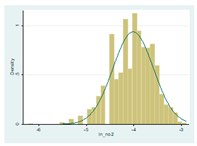
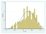
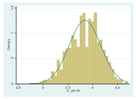
When major variables were evaluated, the mean NO2 concentration was 0.012 ppm, the O3 concentration was 0.027 ppm, and PM10 was 48.93 ug/m3. They were logged and applied to the model and then analyzed using a histogram; the results followed a normal distribution.
In the case of weather variables, the mean temperature was 13.29 °C, the mean wind speed was 2.09 m/s, the mean percentage of sunshine was 50.60%, the mean duration of sunshine was 185.16 h, and the number of yellow dust days was 0.53 on average.
The basic statistics of the variables that consist of source structure and density, independent variables, are as follows. The mean air pollution emission facility density was 0.619 units/m2, the mean registered vehicles per capita was 0.42, the population density over the total area (total population density) was 2155.4 people/km2, and the mean distance to a thermoelectric power plant was 187,058.3 m. Moreover, the vehicle density per unit road was 0.021 units/m2, the mean density of air pollution emission facilities was 926.6 units/km2, and the net population density was 0.021 people/m2.
Since the units of variables are different from each other, an empirical analysis was conducted by using log transformation for conducting analyses consistently.
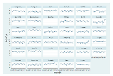
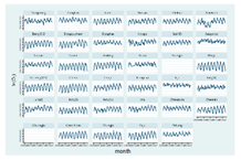
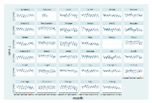
This study prepared panel graphs of air pollution concentration by region (Table 3). Panel graphs were prepared for dependent variables to analyze the meaning and are presented as shown below. NO2 maintained a constant monthly concentration level on a regional basis. O3 showed a steadily increasing trend, and PM10 showed a slight decreasing trend. In the case of NO2, the inter-regional differences were relatively large, and the intra-regional differences were very small except for some regions. On the other hand, the intra-regional differences of O3 were more pronounced than the inter-regional differences of O3. The inter-regional difference showed a high seasonal variation. The difference was relatively large in the season when O3 was relatively high or low. In the case of PM10, inter-regional differences were observed over the entire period, and intra-regional differences were relatively large. In addition, intra-regional differences varied greatly by region.

4.2. Correlation Analysis

A correlation analysis was carried out for variables, and the analysis results are shown in Table 4 and Table 5. Correlations were examined to determine the direction between variables that were set to analyze the influential factors of air pollution concentrations.
The analysis results revealed that the NO2 concentration had a relatively high correlation with the total population density, total emission facility density, percentage of sunshine, monthly precipitation, and the distance to a thermoelectric power plant. The O3 concentration had a relatively high correlation with monthly precipitation, the duration of sunshine, and mean wind speed. PM10 showed a relatively high correlation with monthly rainfall, the percentage of sunshine, and yellow dust.
The monthly precipitation showed a positive correlation with the mean temperature and a negative correlation with the percentage of sunshine. Variables related to densities showed relatively higher correlations than other variables. The total population density had a high correlation with the total emission facility density and the net vehicle density. Moreover, it had a correlation with the net population density and the net emission facility density. Net population density was significantly correlated with total emissions facility density and net vehicle density.
We also calculated correlation coefficients and VIF to resolve the multicollinearity issue of independent variables that may appear when analyzing data using individual variables. In order to judge the independence of independent variables, the multicollinearity of all variables, used for each dependent variable, was tested (Table 4 and Table 5). Pearson’s correlation was used to test multicollinearity. The coefficients of all independent variables except for that between sunshine duration and the percentage of sunshine were below 0.7, the threshold of this study [36,37], indicating there was no multicollinearity issue. Sunshine duration and the percentage of sunshine were used separately while considering the characteristics of a dependent variable due to their multicollinearity.
Analysis of the variance inflation factor (VIF) was performed to confirm stricter variance inflation factor (VIF) values, and the results of the analysis showed that it was below 10, the reference value [38,39,40]. In addition, since it did not exceed 5, the stricter threshold suggested by Hair et al. (2011), it was determined that there was no multicollinearity issue.

4.3. Study Model and Panel Analysis

4.3.1. NO2

The form of the linear regression model used in this study is shown in Table 6.
Model 1 is a model that analyzed the relationship between the NO2 concentration and independent variables for meteorological characteristics. Model 2 added the total population density, vehicle registration per capita, and total emission facility density, which are regional variables among the total density of a source, and Model 3 added the distance to thermoelectric power plant, which is the total density of a source in a broad dimension.
In the next step, the fixed effects and random effects of these three models were estimated and the Chow test, BP test, and Hausman test were performed.
The results of the Hausman test rejected the null hypothesis that there were no systematic difference between the coefficients of Model 1 and accepted the null hypothesis of Model 2 and Model 3. This study selected Models 1 and 4 as fixed effect models and Models 2 and 3 random effect models.
Table 6 shows the analysis results of each model according to the Hausman test.
The analysis results of Model 1 revealed that NO2 concentration had negative relationships with mean temperature, mean wind speed, and monthly precipitation. However, it had a positive relationship with the percentage of sunshine. The effects of meteorological variables on NO2 concentration were in the descending order of mean wind speed, the percentage of sunshine, mean temperature, and monthly precipitation.
Model 2 analyzed the independent variables including local variables among the total source densities. The analysis results showed that the total population density was significant at the 5% level. The total population density had a positive relationship with the NO2 concentration. The number of registered vehicles per capita and NO2 concentration had a positive relationship and the effect was greater. It was found that the total emission facility density had a positive relationship with the NO2 concentration. When regional variables among total source densities were introduced, the magnitude and direction of meteorological characteristics’ effects on the NO2 concentration were not much different from the results of Model 1.
Model 3 added the distance to a thermoelectric power plant, a broad variable among the source structures. The analysis results showed that the NO2 concentration increased with a closer distance to a thermoelectric power plant. In addition, the effects of regional variables among the meteorological characteristics and total source densities on the NO2 concentration were not much different from those in Models 1 and 2.

4.3.2. O3

The form of the linear regression model used in this study is shown in Table 7.
First, Model 1 analyzed the relationship with O3 concentration using independent variables related to meteorological characteristics. Model 2 substituted the duration of sunshine for the percentage of sunshine as a variable related to sunshine, which is associated with photochemical reactions among the weather characteristics. Model 3 added total population density, the number of registered vehicles per capita, and total emission facility density, i.e., regional variables among total source densities. Model 5 added the number of yellow dust days.
In the next step, the fixed effects and random effects of these three models were estimated and the Chow test, BP test, and Hausman test were performed.
Since the results of the Hausman test rejected the null hypothesis that there was no systematic difference between the coefficients of Models 1, 2, 3, and 4, all models of this study were selected as fixed effect models.
Each model was analyzed according to the Hausman test, and the results are shown in Table 7.
The analysis results of Model 1 showed that the O3 concentration had positive relationships with mean temperature, mean wind speed, and the percentage of sunshine. However, monthly mean precipitation was negatively related to O3 concentration. The effects of meteorological variables on O3 concentration were in the descending order of mean wind speed, the percentage of sunshine, mean temperature, and monthly precipitation.
Model 2 added the duration of sunshine instead of the percentage of sunshine. The analysis results showed that O3 concentration had a positive relationship with the duration of sunshine. Moreover, the effects of the duration of sunshine on O3 increased much more than those of the percentage of sunshine, but the effects of mean wind speed decreased.
Model 3 analyzed the independent variables after adding the regional variables among the total source densities. The analysis results showed that the total population density was not significant. The number of registered vehicles per capita was positively related to the O3 concentration and the effect was larger. Total emission facility density and the O3 concentration had a positive relationship. When regional variables among the total source densities were introduced, the effects of mean wind speed on O3 increased and those of the duration of sunshine on O3 decreased compared to Model 2.
Model 4 added the net population density, which is a source net density variable. Analysis results showed that the net population density was negatively related to O3 concentration. In addition, the effects of regional variables among the meteorological characteristics and total source densities on the O3 concentration were not much different from those in Model 3.
Model 5 added the number of yellow dust days among meteorological characteristics. The effects of the number of yellow dust days on O3 were not significant. It was found that, when the number of yellow dust days was controlled, it had stronger inter-regional explanatory power and overall explanatory power compared to Model 4. It was confirmed that the effects of mean wind speed, total source density, and source net density characteristics, showing distinct inter-regional differences, were more robust. In other words, the effects of yellow dust days on ozone were explained more by inter-regional differences when external influences were controlled. Net population density affected the effects of the total source densities and source net density on O3 the most, followed by the number of registered vehicles per capita and total emission facility density.

4.3.3. PM10

The form of the linear regression model used in this study is shown in Table 8. First of all, Model 1 analyzed the relationship with the PM10 concentration using independent variables of the meteorological characteristics.
Model 2 added total population density, total emission facility density, and source density, i.e., regional-dimension variables among the total source densities. Model 3 added the number of yellow dust days among meteorological characteristics.
In the next step, the fixed effects and random effects of these three models were estimated and the Chow test, BP test, and Hausman test were performed.
The results of the Hausman test rejected the null hypotheses that there is no systematic difference between the coefficients of Models 1, 2, 3, and 4. In this study, all models were a fixed effect model.
Each model was analyzed according to the results of the Hausman test (Table 8).
The analysis results of Model 1 revealed that the PM10 concentration increased when mean temperature decreased, mean wind speed increased, the duration of sunshine increased, and monthly precipitation decreased. The effects of meteorological variables on the PM10 concentration were in the descending order of mean wind speed, the duration of sunshine, mean temperature, and monthly precipitation.
Model 2 analyzed the independent variables including regional variables and source density variables among the total source densities. The analysis results showed that total population density and total emission facility density were not significant. On the other hand, the PM10 concentration had positive relationships with net population density, net vehicle density, and net emission facility density, which are source net density characteristics. When regional variables among the total source densities were introduced, the direction and magnitude of the effects of meteorological characteristics on PM10 concentration were not significantly different from Model 1.
Model 3 added the number of yellow dust days among meteorological characteristics. The effect of the number of yellow dust days on PM10 was significant. PM10 concentration was positively related with the number of yellow dust days. By introducing the number of yellow dust days, the effects of mean wind speed on PM10 greatly decreased. Moreover, as the number of yellow dust days was controlled, it revealed that inter- and intra-regional explanatory power and overall explanatory power increased compared to Model 2. The effects of the total source densities and net density characteristics, showing distinctive regional differences, became more robust. In other words, the effects of yellow dust days on ozone were explained better by inter-regional differences because the effects of yellow dust days and external effects were controlled.

4.3.4. Explanation Model for Each Air Pollutant: Panel Model

Table 9 shows the comprehensive results of the final model, selected according to the analysis results of panel models by air pollutant. The detailed analysis results are as follows.
For NO2, a primary pollutant, a random effect model considering inter- and intra-regional differences was selected. This seems to reflect the seasonal changes in pollutant emissions due to energy consumption and the structural characteristics of pollutant sources between regions. On the other hand, O3 and PM10, secondary pollutants, adopted a fixed effect model reflecting intra-regional differences and fluctuations relatively strongly. The results implied that the secondary pollutants were produced through various photochemical reactions in the space, and this was due to complex effects of meteorological characteristics (seasonal effects).
When intra- and inter-subjects effects were compared, these characteristics can be explained in more detail. When the explanatory coefficients of the NO2-total source density model, O3-urban sprawl model, and PM10-source density model were compared, the explanatory coefficients of NO2, PM10, and O3 were 0.457, 0.359, and 0.412, respectively. The explanatory coefficients within regions were 0.333, 0.495, and 0.467 for NO2, PM10, and O3, respectively. The explanatory coefficients between regions were 0.619, 0.353, and 0.154 for NO2, PM10, and O3, respectively. While NO2 was explained better than secondary pollutants by inter-regional differences, secondary pollutants were explained better by intra-regional differences than NO2, a primary pollutant.
When the characteristics of the variables used in this study were evaluated, all meteorological characteristics except for mean wind speed showed large fluctuations or differences within a region, while the differences between regions were minimal. On the other hand, air pollutant total source densities and net density variables showed large differences between regions, but the fluctuations within a region were not large. In the case of NO2, when regional variables among the air pollution total source densities were introduced, the direction and magnitude of the effects of meteorological characteristics on NO2 concentration were not much different from the meteorological characteristics analysis model.
When regional variables among the air pollution total source densities were introduced, the direction and magnitude of the effects of meteorological characteristics on the O3 concentration were found; the mean wind speed increased compared to the model considering only the meteorological characteristics, and the effects of the duration of sunshine decreased. Additionally, when the number of yellow dust days was controlled, inter-regional explanatory power and overall explanatory power increased compared to the model reflecting total source densities and densities. It was confirmed that the effects of mean wind velocity, total source densities, and net density characteristics showing great inter-regional differences became more robust. In other words, the effect of yellow dust days on ozone increases the explanatory power owing to inter-regional differences by controlling external factors.
In the case of PM10, when the number of yellow dust days was controlled, inter- and intra-regional explanatory power and overall explanatory power increased compared to uncontrolled models. It could be confirmed that the effects of total source densities and net density characteristics, showing distinct regional differences, became more robust. In other words, the effects of yellow dust days on ozone were explained better by inter-regional differences as well as the effects of yellow dust days, while external influences were controlled.
Considering the characteristics of these variables and the causal factors of air pollutants, primary and secondary pollutants were derived by regional random effect models and regional fixed effect models, respectively.
On the other hand, PM10 showed a low inter-regional explanatory coefficient (0.154), which was lower than that of other air pollutants (0.154). In the case of NO2 and O3, the effects of inter-regional differences due to the spatial and environmental conditions that can cause photochemical reactions with the source were relatively strong, while PM10 had more complex and diverse influential factors than pollutants. The results of this study showed that the regional and spatial effects of particulate matter were very diverse.

4.4. Discussion

Table 10 shows the results of the hypothesis verification for NO2. NO2 concentration increased when mean temperature decreased, mean wind speed decreased, and monthly precipitation was lower. Moreover, NO2 concentration increased when the percentage of sunshine increased. Therefore, Hypothesis 1.1, expecting the effects of meteorological characteristics on NO2, was accepted. The results of mean temperature were different from those of Cárdenas Rodríguez et al. [8]. The seasonal energy consumption characteristics of South Korea could cause this difference. The main sources of NO2 are automobiles, power plants, and chemical production, which are higher in winter than in other seasons. It could be due to the increase in the heating energy usage in winter. The positive relationship between the percentage of sunshine and NO2 indicated that NO2 concentration would appear to be the highest in spring considering the time series of the percentage of sunshine. In other words, the effect of the percentage of sunshine was a seasonal effect.
It was found that the NO2 concentration increased when the total population density increased. Therefore, Hypothesis 1.2.1, expecting the positive effect of population density (structural characteristic of air pollution sources) on NO2, was supported. These results agreed with Cooper et al. [41] and Requia et al. [42]. However, these results were different from Cárdenas Rodríguez et al. [8], who did not show any influential relationship.
When total emission facility density increased, the NO2 concentration also increased. This supported Hypothesis 1.2.2, which expected to see a positive relationship between NO2 concentration and emission facility density among the source structural characteristics. Previous studies analyzed using the ratio of secondary industry, the area and ratio of industrial area, and the ratio of manufacturing workers, similar to air pollution emission facilities. The results of this study were similar to those of Jung et al. [18]. On the other hand, Cho·Choi [31] and Cárdenas Rodríguez et al. [8] did not show a significant relationship between NO2 concentration and emission facility density.
NO2 concentration increased when the number of registered vehicles per capita increased, and the influence was greater. This supported Hypothesis 1.2.3 arguing that the quantitative increase of cars, a linear pollution source, would increase the NO2 concentration. This supported the claim of the Ministry of Environment [43] that an increase in the number of cars would increase the NO2 concentration in the Air Environment Yearbook. Moreover, the number of registered vehicles per capita is an index reflecting not only the quantitative increase of vehicles but also the economic aspect of a region. When it is connected to the economic power improvement of a region or an individual household, it also indirectly supported Jung et al. [18], who showed that gross regional domestic product(GRDP) and the NO2 concentration were positively related.
This study also added the distance to a thermoelectric power plant, which is a broad variable among air pollution total source densities. The analysis results showed that the NO2 concentration increased at a closer to a thermoelectric power plant. The result statistically proved power plants, emitting gas as a consequence of high temperature combustion, as factors of NO2 production officially claimed by the Ministry of Environment.
All results taken together, the effect of meteorological characteristics on the NO2 concentration seemed to reflect seasonal characteristics. The effects of air pollutant sources, i.e., point and/or linear structure, on NO2 could be due to sociodemographic and economic growth, quantitative increase in automobiles, integration of air pollutant facilities, and proximity to a thermoelectric power plant. In other words, it is believed that NO2 was greatly affected by the emission structural characteristics of air pollutants.
The results of hypothesis verification for O3 are shown in Table 11. O3, a secondary pollutant, was positively related with mean temperature, mean wind speed, monthly precipitation, and the duration of sunshine. These findings supported Hypothesis 2.1 that meteorological characteristics would affect O3 concentration. This relationship could be due to O3 concentration that begins to increase in spring and peaks in summer and the seasonal effects of meteorological characteristics inducing it. The results agreed with Lee [10], who showed the positive relationship between surface temperature and O3. The study also found that the O3 concentration increased when mean wind speed and the duration of sunshine increased. The results could reflect the regional characteristics that increased wind diffusion and photochemical reactions and affected meteorological characteristics. In other words, mean wind speed has relatively higher inter-regional differences than intra-regional differences, unlike other meteorological characteristics. Moreover, the duration of sunshine had relatively larger inter-regional differences. The results suggested that precursors emitted from air pollution sources were diffused by wind or photochemical reactions were activated to increase O3 concentration in areas with high wind speeds.
We believe that the results were due to seasonal and spatial effects. While NO2 is emitted more in the winter due to heating, O3 increases in the summer when photochemical reactions are likely to occur. In Korea, wind speed is generally stronger in the winter than in the summer. Moreover, the mean wind speed, unlike other meteorological variables, has a greater spatial difference than a temporal change. It seems that NO2 is low and O3 increases due to the effects of diffusion as well as seasonal effects in regions with strong wind speeds. In general, NO2 is generated from a line source (although it can be affected by a point source depending on an environment. As a result, there is a concentration gradient of NO2 in the atmosphere. When the wind blows, the concentration can decrease due to dispersion. Contrarily, O3 is mostly generated by photochemical reactions. When PM10 is high in the atmosphere such as in Seoul in South Korea, the wind can clear the sky by dispersing these particles. Consequently, it increases ozone concentration by stimulating photochemical reactions.
When the number of registered vehicles per capita increased, O3 concentration increased (a positive relationship) and the effect was greater, which supported Hypothesis 2.3 that expected a positive relationship between the linear structure of air pollution sources and O3 concentration. The effects of automobiles on O3 have been studied much less than other air pollutants. Cho·Choi [31] analyzed the dependence on automobiles using an index calculated by the number of registered vehicles per capita and road ratio but they reported that this was not significant. The Ministry of Environment [43] mentioned the similarity between the steady increase of O3 concentration and the change trend of the number of registered vehicles based on air pollution status analysis. This study proved this trend analysis statistically.
It was found that the O3 concentration increased when the total emission facility density increased. These results also supported Hypothesis 2.3, which expected a positive relationship between O3 concentrations and the point structure of air pollutant sources. Previous studies did not include air pollution emission facility density as an important factor. Cho·Choi [31] and Lee [10] reported that the relationship was not significant. The Ministry of Environment of Korea [43] reported an increase in the number of registered vehicles as the main causal factor of the increase in O3 concentration but did not mention the density of air pollution emission facilities.
This study did not find a significant relationship between teh O3 concentration and total population density, a structural characteristic of air pollutant sources and an indicator of urban sprawl. The results rejected Hypothesis 2.4.1, which expected a negative relationship between O3 and total population density, one of the characteristics of urban sprawl. These results agreed with Kashem [24] but showed a relationship opposite to Martins et al. [23]. Meanwhile, Lee [10] reported that O3 and population density were not significantly related.
On the other hand, net population density, a variable explaining urban sprawl, negatively affected the O3 concentration. These results supported Hypothesis 2.4.2, which expected a negative relationship between O3 and net population density among urban sprawl characteristics. Cho·Choi [31] confirmed only the quantitative relationship between the net population density and NO2 and CO; the causal relationship for O3 was not significant.
In this study, total population density was not significant in the macroscopic aspect, but net population density representing the activity density or land use intensity of the region had a negative impact on O3. In other words, the effect of the total population density, understood in the concept of urban total quantity, was not identified, while O3 concentration increased when the activity density or the land use intensity of the region decreased. This implies that O3 concentration increases when there are sprawl characteristics decreasing the activity characteristics of the region and land use intensity.
The effects of the number of yellow dust days, one of meteorological characteristics, on O3 was not significant. This could be due to the characteristics of O3. It is known that O3 is greatly influenced by weather factors such as temperature, precipitation, pollutant diffusion, and atmospheric stability in addition to pollutant emissions, and it is produced by photochemical reactions in the atmosphere [43]. These generation characteristics of O3 are different from those of PM10, which is affected by yellow dust. It is believed that the results of this study empirically proved this.
Moreover, since yellow dust days were controlled, it was possible to confirm that the effects of mean wind speed, total source densities, and net density characteristics, showing distinct inter-regional differences, became more robust. The results supported Hypothesis 2.5 that controlling the number of yellow dust days would change the effect of the total source density and net density characteristics of air pollution sources.
It was found that net population density had the largest effects on O3 followed by the number of registered vehicles per capita and total emission facility density among the air pollution total source densities and densities. This may be due to the characteristics of O3 that is affected by air pollutant emissions and the degree of pollutant diffusion. The results of this study may be the empirical analysis of the effects. In particular, it was found that the effects of urban sprawl were larger than those of air pollution total source densities. This implied that it would be important to establish an urban environment and urban space structure that could reduce the reactions between primary pollutants and precursors and their diffusions as well as to manage air pollution sources directly.
As shown in Table 12, the hypothesis test results for PM10 are as follows. First, in terms of meteorological characteristics, PM10 concentration increased when mean temperature decreased, mean wind speed increased, monthly precipitation decreased, and the duration of sunshine increased. This supported Hypothesis 3.1, which expected that meteorological characteristics would affect PM10 concentrations. These results agreed with the results of Cárdenas Rodríguez et al. [8]. On the other hand, Lee [10] did not show any significant relationship. The effects of mean temperature, monthly precipitation, and the duration of sunshine were due to the seasonal effects of PM10. It was observed that mean wind speed and PM10 were positively related. It seems that wind affects the formation of secondary pollutants more than the offset of air pollutants. Increased wind speed in a region seems to have a great effect on the spread of pollutants, and it should be separated from the reduction effects due to changes in the atmosphere.
Total population density and total emission facility density, the structural characteristic of air pollution sources, did not affect PM10 significantly. The results agreed with Cárdenas Rodríguez et al. [8] and Lee [10]. On the other hand, Zou et al. [44] and Kashem [24] showed opposite results, and their results did not concur with the results of this study.
Net population density, among the source net density characteristics, did not significantly affect PM10. These results partially rejected Hypothesis 3.2, which expected a positive effect of air pollution source density on PM10. The results are identical to those of Cho·Choi [31]. On the other hand, net vehicle density and net emission facility density had a positive relationship with the PM10 concentration. This was partly in support of Hypothesis 3.2, which expected a positive relationship between air pollution source density and PM10. Overall, the residents’ activity density or land use intensity (net population density) did not have a significant impact on PM10. However, PM10 concentration increased when the net density of air pollutant sources, indicating the density of air pollution sources or use intensity, increased. It was found that the land use intensity of air pollution sources had a significant effect on the PM10 concentration increase.
It was also found that the number of yellow dust days, one of the meteorological characteristics, significantly influenced PM10. PM10 concentration increased with more yellow dust days. When the number of yellow dust days was introduced, the effects of mean wind speed on PM10 decreased notably. This supported Hypothesis 2.5, which suggested the positive and control effects of yellow dust on the PM10 concentration. It was found that the PM10 concentration increased as the number of yellow dust days increased, and the effects of mean wind speed, which was the only meteorological character showing a positive relationship with the PM10 concentration, also decreased greatly. The results suggested an increase of the external effects of meteorological characteristics affecting PM10 and the decrease of internal effects. Alternatively, the external and internal effects simultaneously affected the PM10 concentration.

5. Conclusions

This study analyzed the effects of density characteristics of air pollution sources on air pollution concentration. This study used a panel model to comprehensively understand the temporal impact (intra-regional differences) and spatial impact (inter-regional differences) of the air pollutants on air pollution. The hypothesis of the research objectives is that source density characteristics, meteorological characteristics, and yellow dust characteristics will affect the concentration of air pollutants differently. A more detailed study hypothesis by air pollutant is as follows. (1) NO2 concentrations will be affected by the total density characteristics of an air pollution source. (2) The O3 will be affected by source structure, urban sprawl characteristics (urban density), sunshine, and yellow dust. (3) PM10 concentration will be affected by the density of sources and yellow dust.
The subjects of this study were 35 municipalities, which provided time-series air pollution concentrations and meteorological data at the same time, among national cities and districts used to establish a Korean panel model. Nitrogen dioxide, ozone, and particulate matter, showing regional differences among air pollutants, were selected as target air pollutants.
Individual previous studies on air pollution and influential factors were reviewed to establish research hypotheses. This study set up a conceptual model in which meteorological characteristics, socioeconomic characteristics, urban density characteristics, urban sprawl characteristics, air pollution source characteristics, and urban land use characteristics would influence air pollution concentrations and there would be inter- and intra-regional differences.
Monthly mean concentration data of NO2, O3, and PM10 for 35 municipalities from 2008 to 2016 were constructed. Moreover, data of independent variables during the same period were also established. The panel model, a statistical technique, was used to test the model using air pollution source characteristics and meteorological characteristics.
The derived results are as follows.
When NO2 was the primary pollutant, a random effect model was adopted considering inter- and intra- regional differences. When total population density increased, the NO2 concentration increased. When the number of registered vehicles per capita increased, the NO2 concentration increased, showing a positive relationship, and the effect was greater. It was found that total emission facility density and NO2 concentrations were positively related. When regional variables among the total source densities were introduced, the direction and magnitude of the effects of meteorological characteristics on the NO2 concentration were not that different from the meteorological characteristics analysis model. The analysis was conducted by adding the distance to a thermoelectric power plant, which is a broad variable among the total source density. It was found that the NO2 concentration increased with a closer distance to a thermoelectric power plant.
The analysis results of O3, a secondary pollutant, revealed that the total population density was not significant. There was a positive relationship between the number of registered vehicles per capita and O3 concentration and the effect was larger. It was observed that when total emission facility density increased, O3 concentration increased. When regional variables among the total source densities were introduced, the direction and magnitude of the effect of meteorological characteristics on O3 concentration were evaluated. It was found that the effects of mean wind speed were larger and the effects of the duration of sunshine were smaller compared to the model considering only the meteorological characteristics. When net population density was introduced and analyzed, O3 concentration increased as net population density decreased. Additionally, the effects of variables showing regional characteristics (urban space sprawl) among the meteorological characteristics and total source densities on O3 concentration were not much different from the causal relationship in the models considering only the total source densities.
When the number of yellow dust days among meteorological characteristics was introduced and analyzed, the effects of the number of yellow dust days on O3 were not significant. However, because the number of yellow dust days was controlled, inter-regional explanatory power and overall explanatory power increased compared to the model reflecting the total source density and net density. It was confirmed that the effects of mean wind speed, total source density, and net density characteristics, which showed distinctive differences between regions, became more robust. In other words, because external effects were controlled, the effects of the number of yellow dust days on ozone were explained more by inter-regional differences. It was found that net population density had the largest effect on O3, followed by the number of registered vehicles per capita and total emission facility density. Based on the analysis results of PM10, analysis was performed for independent variables including regional variables and source density variables. Analysis results showed that total population density and total emission facility density, total source density characteristics, were not significant. On the other hand, the PM10 concentration had positive relationships with net population density, net vehicle density, net vehicle density, and net emission facility density.
Analysis was conducted after adding the number of yellow dust days to find that the effects of the number of yellow dust days on PM10 were significant. The number of yellow dust days was positively related with the PM10 concentration. It can be seen that the impact of mean wind speed on PM10 was greatly reduced by introducing the number of yellow dust days. Additionally, since the number of yellow dust days was controlled, the overall explanatory power and within a region explanatory power increased compared to the uncontrolled model. The effect of the total source density and net density characteristics, with distinctive inter-regional differences, became more robust. In other words, the effects of the number of yellow dust days on ozone had higher explanatory power due to the inter-regional differences when the number of yellow dust days and external influences were controlled.
This study evaluated specific characteristics such as density in terms of variables and methods. Future studies are needed to analyze causal relationships comprehensively. It is necessary to conduct studies to examine the causal relationships for identifying the characteristics of land use, urban structure, and urban environmental changes and for understanding mechanisms. Urban characteristics are very complex processes that are affected by various factors. Therefore, it is necessary to have subdivided indices related to urban characteristics that can reflect the spatial land allocation and industrial and economic characteristics of cities.
The point element measured at a measuring station is used as a representative value of a city for the air pollutant concentration, which is the main interest of this study. In addition, the measurement of the meteorological characteristics measuring station, which is a control variable, is presented as the representative value of a city. On the other hand, the urban air pollution emission spatial density, an independent variable, is an indicator of urban socioeconomic characteristics, land use characteristics, and urban structure characteristics. The data represent the entire space of the city and are a spatial dataset. The differences of spatial hierarchies were integrated into urban units for the analysis of air pollution in terms of urban management. This was for achieving the objective of this study, but it has a limitation of partially including ecological fallacy that leads to conclusions about the individual by observation of the group in the process of data collection and interpretation. Not only this study but also other previous studies actively analyze data at a city unit level to derive the results for urban management. In order to overcome these limitations in the future, it is necessary to construct data on the extent and effect of land use and spatial structure nearby the measuring network in detailed spatial units (e.g., streets) and analyze them. Additionally, future studies need to apply multi-level models and structural equations to analyze the effects of economic characteristics and demographic characteristics, macro units, on air pollution concentrations.
Moreover, air pollutants can cause various health and environmental damage. In other words, human activity, the socioeconomic system, and the environment can result in health issues and various environmental damages, as well as air pollution. In this process, it is necessary to identify the impact structure and role of each factor with respect to health and environmental damage. In particular, we need to analyze the mediated and regulatory effects of air pollution.

Author Contributions

Conceptualization, J.I.B. and Y.U.B.; methodology, J.I.B.; validation, Y.U.B.; formal analysis, J.I.B.; investigation, J.I.B.; writing—original draft preparation, J.I.B. and Y.U.B.; writing—review and editing, Y.U.B.; supervision, Y.U.B. All authors have read and agreed to the published version of the manuscript.

Funding

This research was supported by Basic Science Research Program through the National Research Foundation of Korea(NRF) funded by the Ministry of Education (2020R1A6A3A01100402) and the Ministry of Education of the Republic of the Korea and National Research Foundation of Korea (NRF-2019S1A5B6102699).

Conflicts of Interest

The authors declare no conflict of interest.

References

  1. United Nations. World Urbanization Prospects: The 1996 Revision; United Nations: New York, NY, USA, 2012. [Google Scholar]
  2. Yang, X.; Yue, W.; Xu, H.; Wu, J.; He, Y. Environmental consequences of rapid urbanization in Zhejiang province, East China. Int. J. Environ. Res. Public Health 2014, 11, 7045–7059. [Google Scholar] [CrossRef]
  3. WHO. Ambient (Outdoor) Air Quality and Health; WHO: Geneva, Switzerland, 2014. [Google Scholar]
  4. Tian, Y.; Yao, X.; Chen, L. Analysis of spatial and seasonal distributions of air pollutants by incorporating urban morphological characteristics. Comput. Environ. Urban Syst. 2019, 75, 35–48. [Google Scholar] [CrossRef]
  5. Wei, Y.D.; Ye, X. Urbanization, urban land expansion and environmental change in China. Stoch. Environ. Res. Risk Assess. 2014, 28, 757–765. [Google Scholar] [CrossRef]
  6. Hassan, A.M.; Lee, H. Toward the sustainable development of urban areas: An overview of global trends in trials and policies. Land Use Policy 2015, 48, 199–212. [Google Scholar] [CrossRef]
  7. Bereitschaft, B.; Debbage, K. Urban Form, Air Pollution, and CO2 Emissions in Large, U.S. Metropolitan Areas. Prof. Geogr. 2013, 65, 612–635. [Google Scholar] [CrossRef]
  8. Cárdenas Rodríguez, M.; Dupont-Courtade, L.; Oueslati, W. Air pollution and urban structure linkages: Evidence from European cities. Renew. Sustain. Energy Rev. 2016, 53, 1–9. [Google Scholar] [CrossRef]
  9. Fan, C.; Tian, L.; Zhou, L.; Hou, D.; Song, Y.; Qiao, X.; Li, J. Examining the impacts of urban form on air pollutant emissions: Evidence from China. J. Environ. Manage. 2018, 212, 405–414. [Google Scholar] [CrossRef]
  10. Lee, C. Impacts of urban form on air quality: Emissions on the road and concentrations in the US metropolitan areas. J. Environ. Manage. 2019, 246, 192–202. [Google Scholar] [CrossRef]
  11. Clark, L.P.; Millet, D.B.; Marshall, J.D. Air Quality and Urban Form in U.S. Urban Areas: Evidence from Regulatory Monitors. Environ. Sci. Technol. 2011, 7028–7035. [Google Scholar] [CrossRef]
  12. Kahn, M.E.; Walsh, R. Cities and the Environment. In Handbook of Regional and Urban Economics; Duranton, G., Henderson, J.V., Thisse, J.R., Eds.; Elsevier: Amsterdam, The Netherlands, 2015; Volume 5, pp. 405–465. [Google Scholar]
  13. Huang, Z.; Du, X. Urban Land Expansion and Air Pollution: Evidence from China. J. Urban Plan. Dev. 2018, 144, 05018017. [Google Scholar] [CrossRef]
  14. Chan, C.K.; Yao, X. Air pollution in mega cities in China. Atmos. Environ. 2008, 42, 1–42. [Google Scholar] [CrossRef]
  15. Muralikrishna, I.V.; Manickam, V. Environmental Management: Science and Engineering for Industry, 1st ed.; Butterworth-Heinemann: Oxford, UK, 2017. [Google Scholar]
  16. Marquez, L.O.; Smith, N.C. A framework for linking urban form and air quality. Environ. Model. Softw. 1999, 14, 541–548. [Google Scholar] [CrossRef]
  17. Legras, S.; Cavailhès, J. Environmental performance of the urban form. Reg. Sci. Urban Econ. 2016, 59, 1–11. [Google Scholar] [CrossRef]
  18. Jung, M.C.; Park, J.; Kim, S. Spatial Relationships between Urban Structures and Air Pollution in Korea. Sustainability 2019, 11, 476. [Google Scholar] [CrossRef] [Green Version]
  19. Park, S.H.; Ko, D.W. Investigating the effects of the built environment on PM2.5 and PM10: A case study of Seoul Metropolitan city, South Korea. Sustainability 2018, 10, 4552. [Google Scholar] [CrossRef] [Green Version]
  20. Fang, C.; Liu, H.; Li, G.; Sun, D.; Miao, Z. Estimating the Impact of Urbanization on Air Quality in China Using Spatial Regression Models. Sustainability 2015, 7, 15570–15592. [Google Scholar] [CrossRef] [Green Version]
  21. Frank, L.D.; Sallis, J.F.; Conway, T.L.; Chapman, J.E.; Saelens, B.E.; Bachman, W. Many pathways from land use to health: Associations between neighborhood walkability and active transportation, body mass index, and air quality. J. Am. Plan. Assoc. 2006, 72, 75–87. [Google Scholar] [CrossRef]
  22. Stone, B. Urban sprawl and air quality in large US cities. J. Environ. Manage. 2008, 86, 688–698. [Google Scholar] [CrossRef]
  23. Martins, H.; Miranda, A.; Borrego, C. Urban structure and air quality. In Air Pollution: A Comprehensive Perspective; Budi, H., Ed.; InTech Open: London, UK, 2012. [Google Scholar]
  24. Kashem, S.B.; Irawan, A.; Wilson, B. Evaluating the dynamic impacts of urban form on transportation and environmental outcomes in US cities. Int. J. Environ. Sci. Technol. 2014, 11, 2233–2244. [Google Scholar] [CrossRef] [Green Version]
  25. Mansfield, T.J.; Rodriguez, D.A.; Huegy, J.; Gibson, J.M. The Effects of Urban Form on Ambient Air Pollution and Public Health Risk: A Case Study in Raleigh, North Carolina. Risk Anal. 2015, 35, 901–918. [Google Scholar] [CrossRef] [Green Version]
  26. World Bank. Urban planning and air quality; World Bank: Washington, DC, USA, 2002. [Google Scholar]
  27. Stone, B. Urban Heat and Air Pollution: An Emerging Role for Planners in the Climate Change Debate. J. Am. Plan. Assoc. 2005, 71, 13–25. [Google Scholar] [CrossRef]
  28. Pui, D.Y.H.; Chen, S.-C.; Zuo, Z. PM2.5 in China: Measurements, sources, visibility and health effects, and mitigation. Particuology 2014, 13, 1–26. [Google Scholar] [CrossRef]
  29. Jiang, J.; Zhou, W.; Cheng, Z.; Wang, S.; He, K.; Hao, J. Particulate Matter Distributions in China during a Winter Period with Frequent Pollution Episodes (January 2013). Aerosol Air Qual. Res. 2015, 15, 494–503. [Google Scholar] [CrossRef]
  30. Lu, C.; Liu, Y. Effects of China’s urban form on urban air quality. Urban Stud. 2015, 53, 2607–2623. [Google Scholar] [CrossRef]
  31. Cho, H.S.; Choi, M.J. Effects of compact Urban development on air pollution: Empirical evidence from Korea. Sustainability 2014, 6, 5968–5982. [Google Scholar] [CrossRef] [Green Version]
  32. McCarty, J.; Kaza, N. Urban form and air quality in the United States. Landsc. Urban Plan. 2015, 139, 168–179. [Google Scholar] [CrossRef]
  33. Muttoo, S.; Ramsay, L.; Brunekreef, B.; Beelen, R.; Meliefste, K.; Naidoo, R.N. Land use regression modelling estimating nitrogen oxides exposure in industrial south Durban, South Africa. Sci. Total Environ. 2018, 610–611, 1439–1447. [Google Scholar] [CrossRef]
  34. Kim, D.; Lee, S. A Factor Analysis of Household Gas Demand using Panel Data Model. Seoul City Study 2018, 19, 117–130. [Google Scholar]
  35. Yang, O.-S.; Han, J.-H. The Impact of Research and Development Activities on the Firm Performance in the Emerging Market MNEs: Cost Leadership and Differentiation Strategies. J. CEO Manag. Stud. 2018, 21, 185–208. [Google Scholar]
  36. Anderson, D.R.; Sweeney, D.J.; Williams, T.A. Statistics for Business and Economics; St. Paul West Public Company: West St. Paul, MN, USA, 1996. [Google Scholar]
  37. Griffiths, W.E.; Hill, R.C.; Judge, G.G. Learning and Practicing Econometrics; John Willey and Sons: New York, NY, USA, 1993. [Google Scholar]
  38. Chatterjee, S.; Hadi, A.S. Regression Analysis by Example; John Wiley & Sons: New York, NY, USA, 2015; ISBN 1119122732. [Google Scholar]
  39. Kennedy, P. A Guide to Econometrics, 3rd ed.; MIT Press: Cambridge, MA, USA, 1992. [Google Scholar]
  40. Hair, J.F.; Anderson, R.E.; Tatham, R.L.; Black, W.C. Multivariate Data Analysis, 5th ed.; Prentice-Hall: Englewood Cliffs, NJ, USA, 1998. [Google Scholar]
  41. Cooper, M.; Martin, R.; Donkelaar, A.; Lamsal, L.; Brauer, M.; Brook, J. A Satellite-Based Multi-Pollutant Index of Global Air Quality. Environ. Sci. Technol. 2012, 46, 8523–8524. [Google Scholar] [CrossRef]
  42. Réquia, W.J.; Koutrakis, P.; Roig, H.L. Spatial distribution of vehicle emission inventories in the Federal District, Brazil. Atmos. Environ. 2015, 112, 32–39. [Google Scholar] [CrossRef]
  43. Ministry of Environment. Annual Report on Air Environment; Ministry of Environment, Ed.; Ministry of Environment: Seoul, Korea, 2016. [Google Scholar]
  44. Zou, B.; Xu, S.; Sternberg, T.; Fang, X. Effect of Land Use and Cover Change on Air Quality in Urban Sprawl. Sustainability 2016, 8, 677. [Google Scholar] [CrossRef] [Green Version]
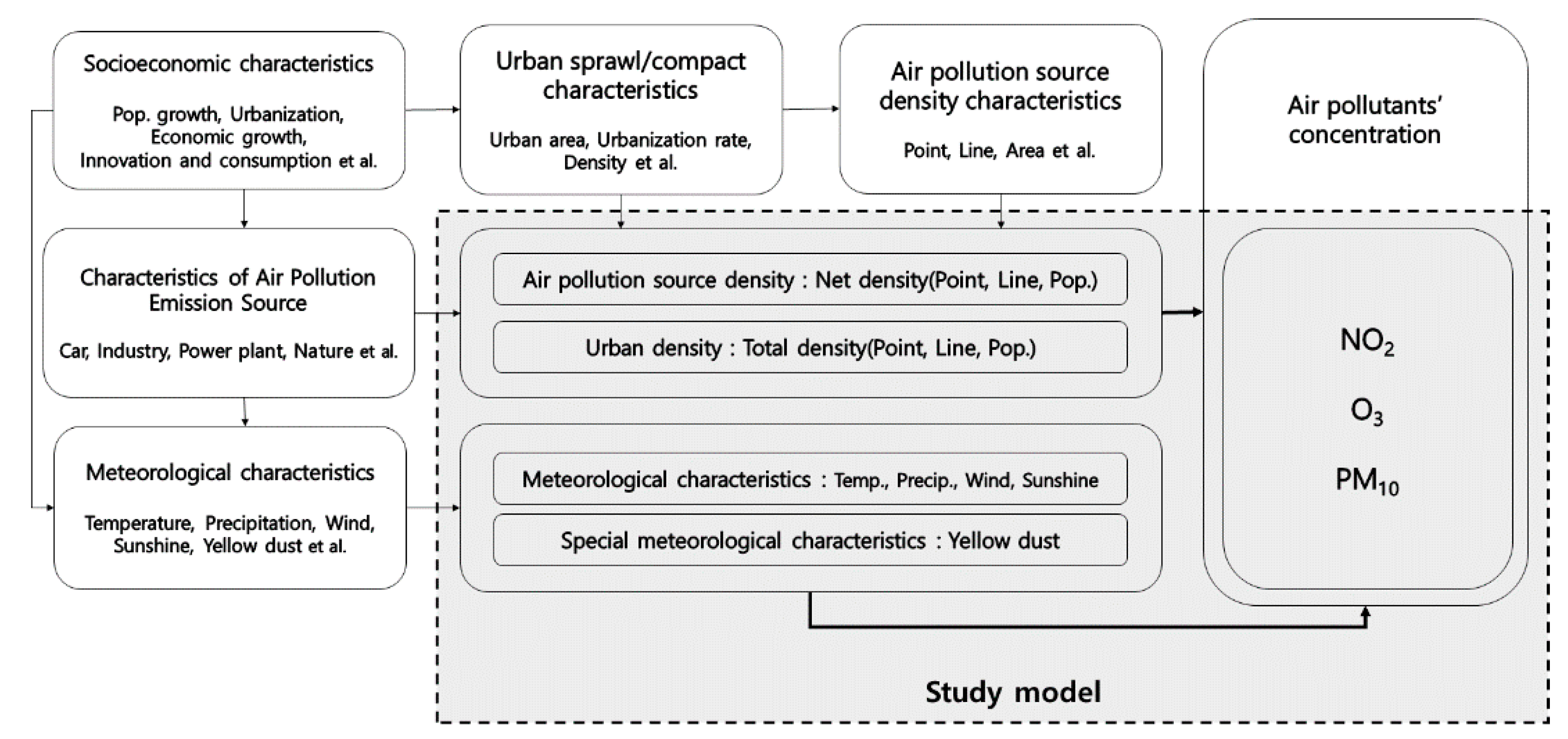
Figure 1. Conceptual model of the research.
Sustainability 12 08401 g001
Figure 2. Geographic location of these 35 municipalities.
Sustainability 12 08401 g002
Figure 3. Analysis process: Panel model.
Sustainability 12 08401 g003
Table 1. Variables Description and data soucre
Variables (Unit)Variable DescriptionSource
Dependent variablesAir
Pollutant
concentration
NO2 (ppm)NO2 monthly
mean concentration
Final confirmed data by monitoring station from Korea Environ-mental Corporation
O3 (ppm)O3 monthly
mean concentration
PM10 (ug/m3)PM10 monthly
mean concentration
Control variablesMeteorological characteristicsMean temperature (°C)Monthly mean temperature Weather observation data
from
the Meteorological Administration
Mean wind speed (m/s)Monthly mean wind speed
Monthly precipitation (mm)Monthly sum of
precipitation
Percent of sunshine (%)Monthly percent of
sunshine
Duration of sunshine (h)Monthly duration of
sunshine
Yellow dust days (day)Monthly yellow dust days
Emission source Distance to a thermoelectric power plant (m)The average distance between the center point of the thermal power plant and the center point of the municipality
Independent variablesUrban densityTotal population density (people/km2)Population/Total areaNational Statistical
Office
Number of registered vehicles per capita (cars)Number of registered vehicles/Population
Total emission facility density (facilities/m2)Number of air pollution emission facilities/Total area
Air pollution source
density
Net population density (people/m2)Population/Residential area
Net vehicle density (cars/m2)Number of vehicles
/Road area
Net emission facility density (facilities/m2)Number of air pollution emission facilities/Factory area
TimeAir pollutant concentration, Meteorological characteristics: Monthly average (2008~2016)
Urban density, Air pollution source density: Annual average (2008~2016)
Table 2. Descriptive statistics table.
VariablesObs.MeanStd. Dev.Min.Max.
NOverall
n Between
T-bar Within
Dep.Air
pollutant
concentration
NO2 (ppm)37710.0200.0080.0020.055
35 0.0060.0100.036
107.7 0.0060.0270.059
O3 (ppm)37590.0270.0100.0070.061
35 0.0040.0200.038
107.4 0.0090.0090.059
PM10 (ug/m3)369248.9315.2815111
35 6.5338.9366.47
105.5 13.8410.76112.01
ControlMeteorological
characteristics
Mean temperature (℃)377813.299.43−10.629.3
35 1.4011.0716.94
107.9 9.33−8.3829.42
Mean wind speed(m/s)37782.090.770.705.90
35 0.661.194.00
107.9 0.410.704.41
Monthly precipitation (mm)3777108.08125.301223.5
35 16.9381.47177.36
107.9 124.2001,211.50
Percent of sunshine (%)377950.6012.459.1679.92
35 3.1338.7455.73
107.9 12.0613.9278.57
Duration of sunshine (h)3779185.1644.5628.4316.6
35 10.45146.64202.89
107.9 43.3543.89316.79
Yellow dust days(day)30360.551.79074
32 0.160.361.17
94.9 1.78073.39
Emission source Distance to a thermoelectric power plant (m)3780187,058.3120,228.39693.9479,723
35 121.967.99693.9479,723
108 0.00187,058.3187,058.3
IndependentUrban densityTotal population density (people/km2)37802155.43764.3110.017,576.2
35 3789.8111.016,904.2
108 462.4721.57151.0
Number of registered vehicles per capita(cars)37800.420.060.310.73
35 0.040.340.54
108 0.040.300.61
Total emission facility density (facilities/m2)37800.620.8607.42
35 0.700.083.74
108 0.5106.43
Air pollution source
density
Net population density (people/m2)37800.0210.0200.0070.127
35 0.0200.0070.125
108 0.0010.0150.030
Net vehicle density (cars/m2)37800.0210.0400.0040.645
35 0.0240.0050.113
108 0.03200.552
Net emission facility density (facilities/km2)3672926.67475.64.8980,645.2
34 4492.98.0426,082.0
108 6023.9055,489.8
Sustainability 12 08401 i001 Sustainability 12 08401 i002 Sustainability 12 08401 i003
Ln (NO2)Ln (O3)Ln (PM10)
Histogram: Dependent variable
Table 3. Panel graph of dependent variables by region.
ln(NO2)ln(O3)ln(PM10)
Sustainability 12 08401 i004 Sustainability 12 08401 i005 Sustainability 12 08401 i006
Table 4. Simple Correlation Analysis by Variables and VIF (continued).
Ln (NO2)ln(O3)Ln (PM10)Ln (Mean Temperature)Ln (Mean Wind Speed)Ln (Monthly Precipitation)Ln (Percent of Sunshine)VIF
NO2O3PM10
Ln (Mean temperature)−0.3757 * 0.4310 * −0.4135 *1 1.461.611.61
Ln (Mean wind speed−0.0125 0.2846 * −0.0567 * −0.1121 *1 1.171.291.30
Ln (Monthly precipitation)−0.3749 * 0.3321 * −0.4453 * 0.5345 * 0.0045 1 1.941.731.73
Ln (Percent of sunshine)0.3386 * −0.0384 * 0.3483 * −0.2949 * 0.0830 * −0.5644 *11.53
Ln (Duration of sunshine) 0.1213 * 0.3215 * 0.2166 * 0.0645 * 0.0935 *−0.2716 *0.8600 * 1.251.25
Ln (Yellow dust days)−0.0764 *0.1502 *0.2778 *−0.05980.1393 *0.0781 *−0.1437 *1.141.151.15
Ln (Total population density)0.4389 *−0.1105 *0.0211−0.00110.2304 *0.01980.0754 *1.932.133.64
Ln (Number of registered vehicles per capita)−0.0565 *0.1682 *0.1682 *0.02560.0941 *0.0535 *0.01871.101.13
Ln (Total emission facility density)0.3917 *−0.0908 *0.0920 *−0.00690.0349 *−0.00420.0886 *1.961.992.22
Ln (Distance to a thermoelectric power plant)−0.3346 *0.2159 *−0.1852 *0.01040.1718 *0.1060 *−0.0519 *1.22
Ln (Net population density)0.1781 *−0.1243 *0.2222 *0.0094−0.1504 *−0.02630.0349 * 1.821.76
Ln (Net vehicle density)0.2973 *−0.0864 *0.0808 *0.00010.1617 *−0.00800.0626 * 1.92
Ln (Net emission facility density)0.2187 *−0.1242 *0.0894 *0.0240−0.0038−0.0044−0.0150 1.43
Table 5. Simple Correlation Analysis by Variables and VIF.
Ln (Duration of Sunshine)Ln (Yellow Dust Days)Ln (Total Population Density)Ln (Number of Registered Vehicles Per Capita)Ln (Total Emission Facility Density)Ln (Distance to a Thermoelectric Power Plant)Ln (Net Population Density)Ln (Net Vehicle Density)VIF
NO2O3PM10
ln_s_sun_du 1 1.251.25
ln_d_hs0.1283 *1 1.141.151.15
ln_pop_den0.0804 *0.0515 *1 1.932.133.64
ln_pc_car0.0186−0.0569 * −0.2130 *1 1.101.13
ln_den_ef_a0.0924 *0.02910.6528 *−0.0923 *1 1.961.992.22
ln_di_plant−0.0548 *−0.0468 *−0.1377 *0.0152−0.2513 *1 1.22
ln_pop_net_den0.0379 *0.0454 *0.4370 *−0.2885 *0.4018 *−0.2953 *1 1.821.76
ln_den_car_r0.0670 *0.0558 *0.6955 *-0.03170.3652 *−0.2082 *0.4702 *1 1.92
ln_den_ef_f−0.015 0.0403 *0.4128 *−0.0406 *0.1052 *−0.2215 *0.2491 *0.3666 * 1.43
Table 6. Regression model: NO2.
ModelEquation
1 ln N O 2 = α 0 + β 1 lnTP + β 2 ln W B + β 3 ln M P + β 4 ln S R + ε
2 ln N O 2 = α 0 + β 1 lnTP + β 2 ln W B + β 3 ln M P + β 4 ln S R + β 5 ln P D + β 6 ln P C C + β 7 ln D E A + ε
3 ln N O 2 = α 0 + β 1 lnTP + β 2 ln W B + β 3 ln M P + β 4 ln S R + β 5 ln P D + β 6 ln P C C + β 7 ln D E A + β 8 ln D P + ε
TP: Mean temperature, WB: Mean wind speed, MP: Monthly precipitation, SR: Percent of sunshine. PD: Total population density, PCC: Number of registered vehicles per capita, DEA: Total emission facility density, DP: Distance to a thermoelectric power plant.
Table 7. Regression model: O3.
ModelEquation
1 ln O 3 = α 0 + β 1 lnTP + β 2 ln W B + β 3 ln M P + β 4 ln S R + ε
2 ln O 3 = α 0 + β 1 lnTP + β 2 ln W B + β 3 ln M P + β 4 ln S D + ε
3 ln O 3 = α 0 + β 1 lnTP + β 2 ln W B + β 3 ln M P + β 4 ln S D + β 5 ln P D + β 6 ln P C C + β 7 ln D E A + ε
4 ln O 3 = α 0 + β 1 lnTP + β 2 ln W B + β 3 ln M P + β 4 ln S D + β 5 ln P D + β 6 ln P C C + β 7 ln D E A + β 8 ln P N D + ε
5 ln O 3 = α 0 + β 1 lnTP + β 2 ln W B + β 3 ln M P + β 4 ln S D + β 5 ln P D + β 6 ln P C C + β 7 ln D E A + β 8 ln P N D + β 9 ln Y D + ε
TP: Mean temperature, WB: Mean wind speed, MP: Monthly precipitation, SR: Percent of sunshine, SD: Duration of sunshine, PD: Total population density, PCC: Number of registered vehicles per capita, DEA: Total emission facility density, PND: Net population density, YD: Yellow dust days.
Table 8. Regression model: PM10.
ModelEquation
1 ln P M 10 = α 0 + β 1 lnTP + β 2 ln W S + β 3 ln M P + β 4 ln S D + ε
2 ln P M 10 = α 0 + β 1 lnTP + β 2 ln W S + β 3 ln M P + β 4 ln S D + β 5 ln P D + β 6 ln D E A + β 7 ln P N D + β 8 ln C N D + β 9 ln E N D + ε
3 ln P M 10 = α 0 + β 1 lnTP + β 2 ln W S + β 3 ln M P + β 4 ln S D + β 5 ln P D + β 6 ln D E A + β 7 ln P N D + β 8 ln C N D + β 9 ln E N D + β 10 ln Y D + ε
TP: Mean temperature, WB: Mean wind speed, MP: Monthly precipitation, SD: Duration of sunshine, PD: Total population density, DEA: Total emission facility density, PND: Net population density, CND: Net vehicle density, END: Net emission facility density, YD: Yellow dust days.
Table 9. Panel analysis results.
VariablesNO2O3PM10
1 (FE)2 (RE)3 (RE)1 (FE)2 (FE)3 (FE)4 (FE)5 (FE)1 (FE)2 (FE)3 (FE)
Meteorological characteristicsLn (Mean temperature)−0.135 ***−0.135 ***−0.134 ***0.204 ***0.153 ***0.160 ***0.161 ***0.163 ***−0.089 ***−0.091 ***−0.078 ***
Ln (Mean wind speed)−0.184 ***−0.168 ***−0.164 ***0.675 ***0.578 ***0.617 ***0.618 ***0.623 ***0.314 ***0.312 ***0.134 ***
Ln (Monthly precipitation)−0.043 ***−0.047 ***−0.047 ***−0.025 ***0.045 ***0.039 ***0.039 ***0.006 ***−0.067 ***−0.067 ***−0.051 ***
Ln (Percent of sunshine)0.169 ***0.161 ***0.161 ***0.286 ***
Ln (Duration of sunshine) 0.493 ***0.463 ***0.461 ***0.472 ***0.208 ***0.216 ***0.191 ***
Ln (Yellow dust days) 0.001 0.034 ***
Emission sourceLn (Distance to a thermoelectric power plant) −0.099 ***
Urban densityLn (Total population density) 0.090 **0.090 *** −0.053−0.057−0.054 −0.046−0.056
Ln (Number of registered
vehicles per capita)
0.129 ***0.134 *** 0.420 ***0.400 ***0.282 ***
Ln (Total emission facility density) 0.049 ***0.046 *** 0.043 **0.047 **0.070 *** −0.0000.018
Air pollution source
density
Ln (Net population density) −0.401 ***−0.319 *** 0.258 ***0.133
Ln (Net vehicle density) 0.058 ***0.040 ***
Ln (Net emission facility density) 0.041 ***0.025 **
Statistical resultsConstant−4.076 ***−4.474 ***−3.302 ***−5.817 ***−7.159 ***−6.248 ***−7.872 ***−7.720 ***3.024 ***5.015 ***4.681 ***
Observation33873316331633753375330433042663332032132636
N. groups3535353535353532353431
R2within
between
overall
0.326
0.003
0.170
0.333
0.558
0.415
0.333
0.619
0.457
0.395
0.122
0.264
0.477
0.096
0.343
0.495
0.221
0.400
0.498
0.186
0.279
0.495
0.353
0.359
0.351
0.192
0.163
0.368
0.050
0.257
0.467
0.154
0.412
Σu0.2970.2020.1820.2010.1840.1760.2900.2390.1820.1680.126
Σe0.2550.2550.2550.2660.2480.2440.2440.2440.2370.2350.216
ρ0.5760.3850.3380.3640.3560.3420.5870.4900.3730.3390.253
Test
results
F-test120.63 ***55.52 ***55.52 ***32.03 ***36.67 ***25.23 ***24.86 ***24.48 ***28.79 ***20.14 ***16.16 ***
Breusch–Pagan test43298.15 ***19652.51 ***14138.97 ***5750.20 ***8650.81 ***4182.74 ***3950.23 ***3756.80 ***3919.38 ***1878.00 ***1498.01 ***
Hausman test10.43 **12.9613.4659.31 ***49.01 ***53.37 ***73.69 ***44.58 ***55.25 ***50.56 ***19.48 **
Wald test1618.87 ***1671.62 ***1687.47 ***2095.46 ***2963.60 ***3121.52 ***3123.43 ***2511.42 ***1702.72 ***1791.99 ***2282.02 ***
* < 0.05, ** < 0.01
Table 10. Hypothesis verification results: NO2.
HypothesisExpectationResult
Hypothesis 1.1 (H1.1).Meteorological characteristics will affect NO2 concentrations.−, +Accept
Hypothesis 1.2.1 (H1.2.1).Population density will have a positive impact on NO2 concentrations.+Accept
Hypothesis 1.2.2 (H1.2.2).Total emission facility density, point air pollution source will have a positive impact on NO2 concentrations.+Accept
Hypothesis 1.2.3 (H1.2.3).Cars, a linear pollution source will have a positive impact on NO2 concentrations.+Accept
Hypothesis 1.3 (H1.3).NO2 concentration will increase when it is closer to a thermoelectric power plant.Accept
Table 11. Hypothesis verification results: O3.
HypothesisExpectationResult
Hypothesis 2.1 (H2.1).O3 concentrations will be affected by meteorological characteristics.−, +Accept
Hypothesis 2.2 (H2.2).Sunlight time affecting photochemical reactions will have a positive impact on the O3 concentration.+Accept
Hypothesis 2.3 (H2.3).Cars and emission facilities will have a positive impact on O3 concentrations.+Accept
Hypothesis 2.4.1 (H2.4.1).The total population density will have a negative impact on the O3 concentration.Reject
Hypothesis 2.4.2 (H2.4.2).Net population density will have a negative impact on O3 concentration.Accept
Hypothesis 2.5 (H2.5).Yellow dust, an external meteorological characteristic, will have a positive impact on O3 concentrations. Moreover, when the yellow dust effect is controlled, the impact of other factors on the O3 concentration will vary.+/ChangeReject/Reject
Table 12. Hypothesis verification results: PM10.
HypothesisExpectationResult
Hypothesis 3.1 (H3.1).Meteorological characteristics will affect PM10 concentrations.−, +Accept
Hypothesis 3.2.1 (H3.2.1).The density of the air pollutant sources will have a positive impact on PM10 concentrations.+Reject
Hypothesis 3.2.2 (H3.2.2).Net population density and net density (density) of cars and air pollution source facilities will have a positive impact on PM10 concentrations.+Partially accept
(Emission facility, Number of registered vehicles per capita)
Hypothesis 3.3 (H3.3).Yellow dust will have a positive impact on PM10 concentrations.+/ChangeAccept/
Partially accept (Net pop. den.)