Methods for Downscaling National Material Consumption Data to the Regional and Municipal Levels

Abstract

Decision makers are looking to reach consumption-based environmental impact targets like Sustainable Development Goal 12, Responsible Consumption and Production. These goals require multifaceted action at municipal, regional, and national levels; however, there are limitations to calculating consumption at the regional and municipal levels. Consumption is dependent on the socioeconomic metabolism of the area, with its unique composition of industries, consumers, and public facilities, which may affect the most appropriate measures to meet goals effectively. In this study, we evaluated several methods to extrapolate municipality- and region-specific consumption from national-level data so that consumption estimates can be used to aid decision makers or make further analyses like environmental impact evaluation. We compared four approaches and validated our findings using reported consumption values as well as results from another model in use. We found that using per capita values for consumption is satisfactory for counties, but consumption in municipalities and metropolitan areas with populations smaller than 500,000 inhabitants was better described by one of the suggested methods on average.

1. Introduction

Rising consumption is leading to increasing resource use and detrimental environmental impacts [1]. Meanwhile, decision makers at all governmental levels are faced with the challenge of defining measures to reach environmental targets and reduce environmental impacts of consumption. For example, the United Nations Sustainable Development Goal (SDG) 12, Sustainable Consumption and Production, has a target of achieving sustainable management and efficient use of natural resources by 2030 [2,3]. This goal is measured against several indicators, including material footprint and domestic material consumption (DMC). Moreover, the SDGs are expected to be met through actions at all governmental levels [4]. In order to successfully reduce consumption and find relevant priority product groups, it may be helpful to quantify regional consumption levels so that targets are region-appropriate [5]. Region-specific consumption data may be key to identifying suitable strategies to reach sustainability goals. In this study, we use the term region to mean a geographic area smaller than the national level, like a county or municipality.

There are challenges to quantifying region-specific consumption values, including data scarcity and uncertainties as well as data confidentiality issues. Data can be expensive to procure. Many consumption quantification efforts produce results at the national level, often based on economic or expenditure data, which are then extrapolated to the regional level using per capita values [6] or applied to specific consumer types (e.g., households) [7,8]. Household consumption may also be quantified through household budget surveys [9,10]. Some may use bottom-up assessment [11] or a mix of top-down and bottom-up methods [12,13,14,15], often using multiregional input–output tables [16,17]. In rare cases, region-specific economic data are used to quantify region-specific consumption and its impact [18,19]. Although per capita values are often used to downscale national values to the local level, these values may be misleading as urban and rural areas may have different consumption patterns [11,20]. Moreover, urban areas have been shown to have different consumption patterns based on their profile (e.g., industrial, service-based), which may indicate a need for more region-specific extrapolations [21].

Two keys to meeting the SDGs would be to (1) identify materials or products that are consumed in such quantities that reduction in their consumption would make a material difference and then (2) identify measures that the region can take, encourage, or require that will reduce the quantity of consumption [22]. Identifying these materials in a rigorous way can be a time-consuming and expensive process that can test the resources of the region. The purpose of this investigation is to search for proxies for more detailed analysis that are sufficiently accurate to enable effective decision making within existing financial and time constraints.

To this end, we investigated four alternative methods of downscaling national-level consumption data to different regional levels. Three of the investigated methods connect several economic sectors to each product type. We tested the use of the number of employees working within those sectors in the region to extrapolate from national DMC to regional levels. We then compared those values to consumption results using per capita values (the fourth method) as well as to reported regional consumption values for certain product types. Our aim was to identify a simple method to downscale national-level data to the local level, and, using products where such data are available, to see if the values produced are close enough to the reported values to indicate that use of the method would enable good decision making at a lower cost.

2. Materials and Methods

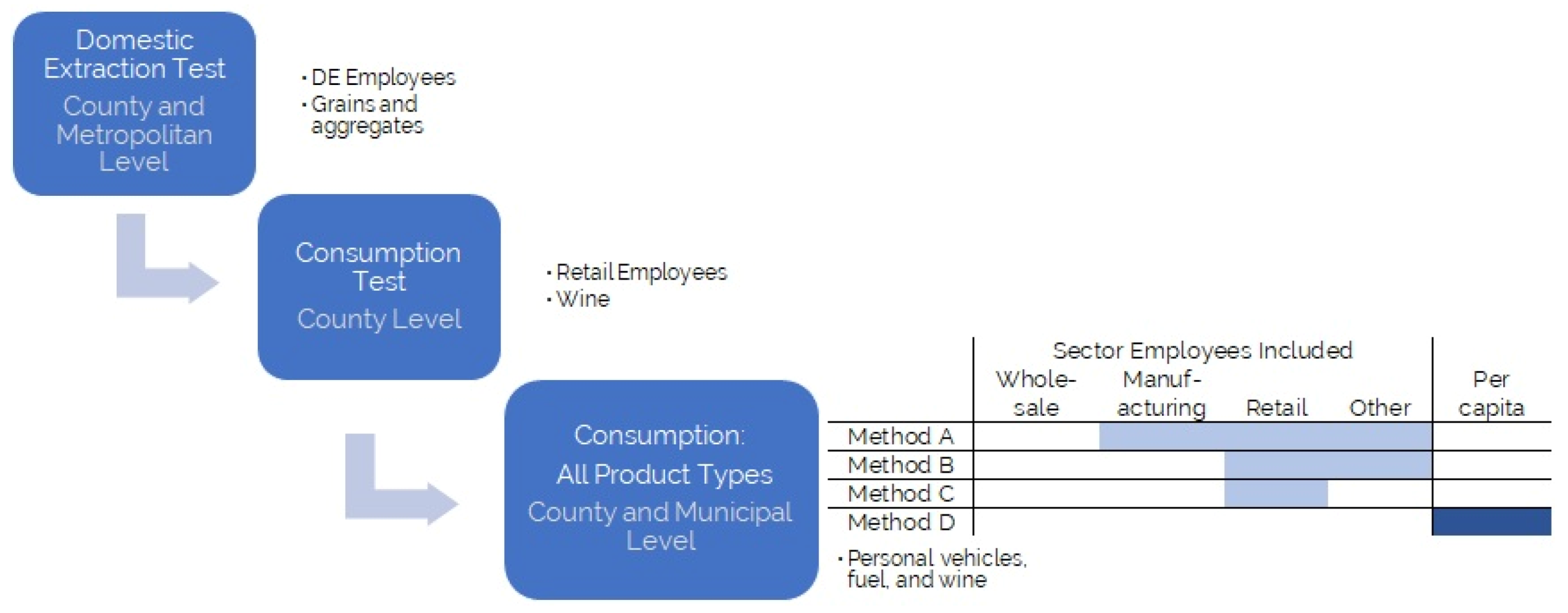
The investigation in this paper was performed by testing different options for extrapolating national consumption data to the regional level. To do so, several steps were needed; each step is described in detail in the following subsections and presented in Figure 1.

Our first aim was to evaluate the use of employees as a suitable proxy for downscaling national levels. We tested using the number of employees working in domestic-extraction-related economic sectors in a region to extrapolate the domestic extraction (DE) for that region from national level data. The benefit of using DE was that reported values of extraction at the national, county, and metropolitan scales are available. Using these data, we could see at which scale(s) it is possible to base the estimate of extraction on the number of employees.

Then, we tested whether we could use the number of retail employees to estimate the consumption of a specific product for which we had the reported values of consumption at the county level. Finally, we downscaled national consumption for the year 2010 (1212 product types) to the county and municipal levels using three different sets of employee types and compared the results to per capita values as well as reported values for certain products, including personal vehicles and fuel.

2.1. Terminology

In this paper we refer to several nomenclatures. The statistical classification of economic activities in the European Community (NACE) provides a four-digit code for economic activities, where the first two digits describe the economic activity category and the second two digits provide more specificity (e.g., NACE category 52 is retail trade, NACE code 5242 is retail sale of clothing). In this paper, we use version Rev 1.1 (2002) [23].

The combined nomenclature (CN) is a system of codes used to classify goods for import and export, used for trade statistics and custom duties [24], where the first two digits indicate the product category (e.g., 04 is dairy), the next two digits indicate the product type (e.g., 0406 is cheese and curd), and the final four digits add specificity (04064050 is Gorgonzola). The CN corresponds to the Harmonized System used in the United States for trade. The DMC is reported in CN codes and provides annual data on consumed materials and goods at the national level. DMC includes raw materials, intermediate goods, and final goods. All of the extrapolation methods performed in this paper use final goods that have been transformed from raw or intermediate materials using the Urban Metabolism Analyst (UMAn) method [25], but any transformation method would be acceptable.

The European Union uses the Nomenclature of Territorial Units for Statistics (NUTS), where NUTS1 represents major socioeconomic regions, NUTS2 defines basic regions for application of regional polices, and NUTS3 represents smaller regions for specific diagnoses [26].

2.2. Extrapolation of Domestic Extraction from Number of Employees

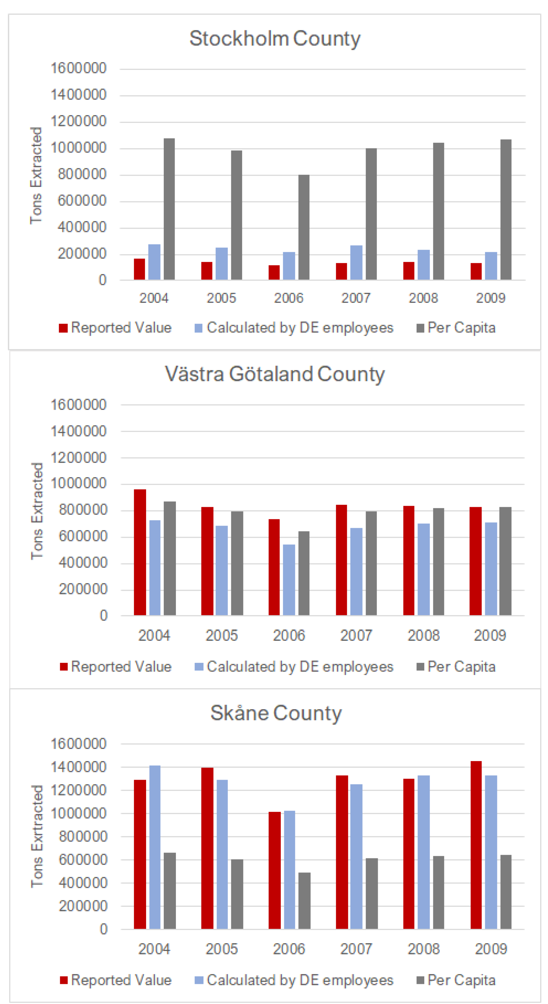
Domestic extraction is the amount of raw material extracted from the natural environment for use in the economy [27]. Globally, as much as 90% of DE is used domestically [28]; in Sweden, the quantities of extraction are documented by Statistics Sweden (SCB) by region. We estimated regional DE values using winter wheat, spring barley, and construction aggregates, as these are products that were extracted in all regions in Sweden. Data at the county and national level for the years 2004 through 2009 were used.

The numbers of employees working in either agriculture (NACE code 0111, “growing of cereals”) or quarrying/gravel extraction (NACE code 1421, “operation of gravel and sand pits”) within each respective NACE code for each metropolitan area and region (NUTS3) and for the country as a whole were found using national statistics. The share of national employees working in each NACE code in each region was calculated (the “employee ratio”) as shown in Equation (1).

$$E{R}_{n,r}= \frac{E_{n,r}}{E_n}$$

(1)

where ER_n,r is the employee ratio for NACE sector n and region r, E_n,r is the number of employees for NACE sector n and region r, and E_n is the total number of employees in the country for NACE sector n.

$${\displaystyle \sum }_r{E}_{n,r}= E_n ; {\displaystyle \sum }_{r}E{R}_{n,r}= 1$$

The total masses of winter wheat, spring barley, and aggregates extracted nationally were multiplied by the employee ratio for each geographical region, as shown in Equation (2), and compared to reported values extracted within the region as well as to per capita values.

$$D{E}_{n, r}=E{R}_{n,r}\times D{E}_n,$$

(2)

where DE_n,r is domestic extraction for NACE sector n and region r, ER_n,r is the employee ratio for NACE sector n and region r, and DE_n is total domestic extraction in the country for NACE sector n.

$${\displaystyle \sum }_{r}D{E}_{n,r}= D{E}_n$$

2.3. Extrapolation of Product Consumption from Number of Employees

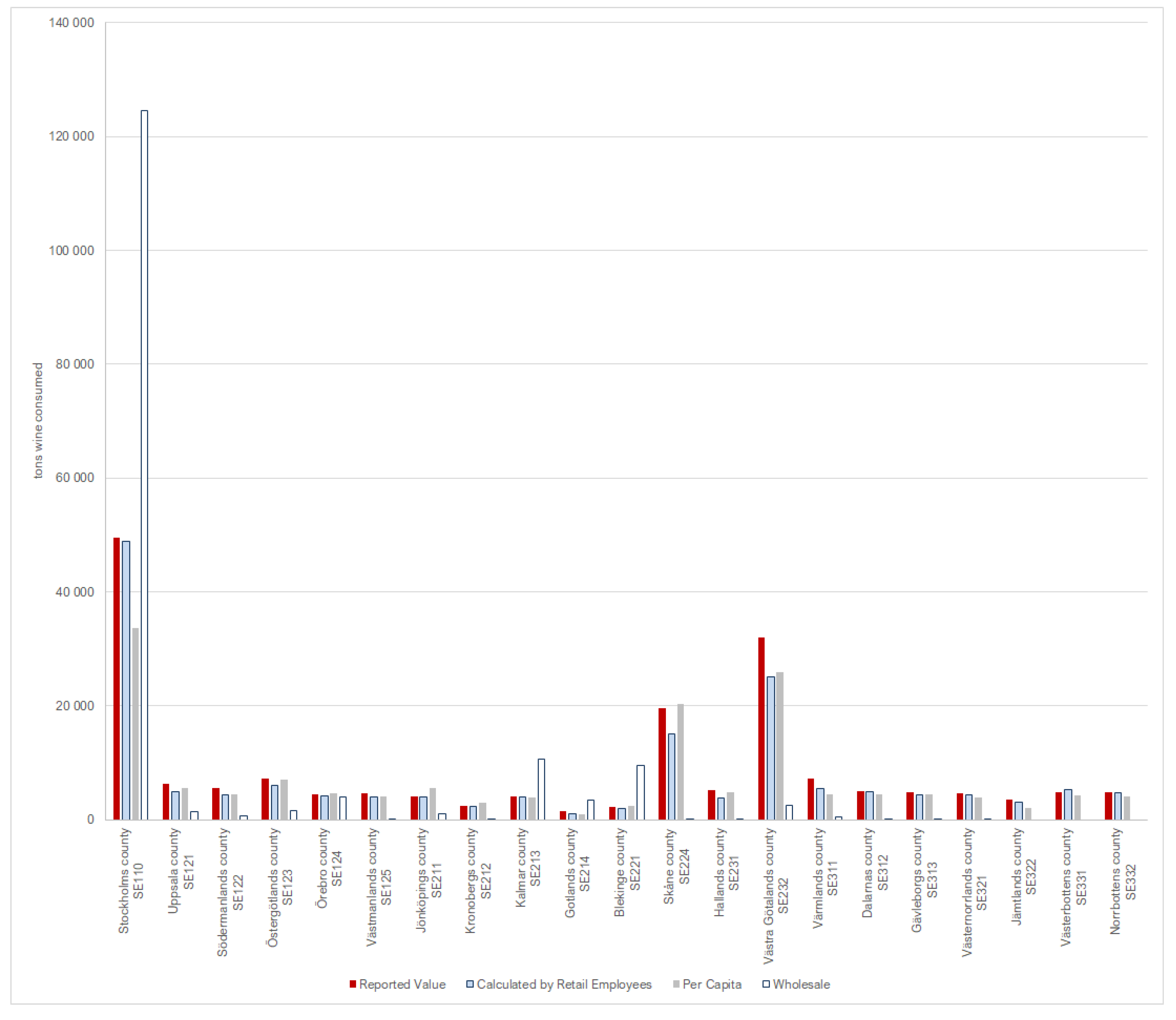
We next assessed whether employees could be used to estimate consumption (Equation (3)). To test this, we first evaluated one product that is primarily imported and for which we have reported values of consumption. The sale of alcohol is regulated and limited to sale by a single, state-owned retailer in Sweden, which allows for accurate data availability. Wine falls under the category of alcoholic beverages and is mostly imported. The DMC of wine (CN2204) for the year 2010 was extrapolated to the regional (county) level using the employee ratio for employees working in NACE code 5225, “retail sale of alcoholic and other beverages”, and compared to reported values consumed at the regional level published by the Swedish Public Health Administration.

$$C_{x,r}=E{R}_{n,r}\times DM{C}_x$$

(3)

where n = appropriate for product x sector, C_x,r is the consumption of product x by NACE sector n in region r, ER_n,r is the employee ratio for NACE sector n and region r, and DMC_x is the total domestic consumption of product x by NACE sector n in the country.

$${\displaystyle \sum }_r{C}_{x,r}= DM{C}_n$$

2.4. Extrapolation of Total Regional Consumption

Expanding the extrapolation method using employees required two steps: (1) transforming DMC into final goods, described in Section 2.4.1, and (2) associating CN product types with NACE economic sectors, described in Section 2.4.2. The regional employee ratio of each economic sector was then used to extrapolate national-level consumption to the region of interest, described in Section 2.4.3. We also extrapolated regional consumption using per capita values, described in Section 2.4.4. The extrapolation was performed at both the county and municipal levels.

All extrapolations were summed to find the total tonnage of all consumption in the region. This was done with the intention of seeing if any of the methods resulted in outliers or unusual results. The extrapolated values were also compared to known values of consumption for specific products. These reported values were primarily collected through Statistics Sweden (SCB). Reported values included personal vehicles (CN code 8703), based on the number of newly registered vehicles in each county or municipality, multiplied by the average mass of a personal vehicle in Sweden in 2010 (1400 kg) [29,30]. Total volumes of delivered fuel (CN code 2710) are also collected at the county and municipal levels. These volumes were converted to tons using density and compared to the extrapolated values. Reported values for wine consumption (CN code 2204), as described in Section 2.3, were available at the county level.

2.4.1. Transformation of Products into Final Goods

National statistics offices collect DMC data; however, product data are often in the raw or intermediate state. For example, while values of aluminum consumption are reported, the identity of products produced (like automobiles) from the consumed aluminum are not reported. Transformed DMC, where DMC has been transformed into final goods, must be used for this step to get an accurate understanding of what is being consumed.

We used national-level results from the Urban Metabolism Analyst (UMAn) model for Sweden [21,25,31], where DMC is transformed into final goods using production and transport data. The model quantifies final good DMC by calculating domestic extraction plus imports, minus exports, using statistical transport and trade data. Transformation of raw goods and intermediate products into final goods is based on the economic activities found in the area of study. Final goods are categorized using the CN. The UMAn model results used were for the year 2010, as this was the most recent year available with corresponding reported values. Any transformation method can be used, however, and the extrapolation methods assessed in this paper are not limited to the UMAn model.

2.4.2. Identifying Relevant Economic Sectors for Product types

In this step, we linked CN4 product types to NACE economic sectors using international trade statistics. There are over one thousand products at the CN4 level, and there is no current linkage between the two nomenclatures. To identify the economic sector that sells or uses the good manually would be inefficient and subjective. Trade statistics report which NACE codes import which CN products, which means that trade data can be used to identify this link. Since we are investigating consumption, the relevant NACE codes are those that represent the end of the supply chain prior to consumption, and thus a selection of suitable NACE codes was necessary. For example, wholesale companies are often centralized and not located in all regions, but they are often responsible for importing goods. Results are likely to be misleading if national consumption is extrapolated to the regional level using values based on wholesale imports. Wholesale employees have therefore been excluded from this analysis.

Moreover, many importing economic sectors are manufacturers and are thus also not responsible for the end of the supply chain. With these uncertainties in mind, we tested three alternatives for identifying the most appropriate NACE code for each CN4 product type:

• Method A: Use all economic sectors with the exception of wholesale (i.e., use all NACE codes except for those in category “51”).
• Method B: Use all economic sectors with the exception of wholesale and manufacturing (i.e., use all NACE codes except for those in categories “01” through “36” and “51”).
• Method C: Use only retail economic sectors (i.e., any NACE codes in categories “50” or “52”).

Some CN codes are linked to several NACE codes. In these cases, the mass of the CN4 was allocated to each NACE code using the import ratios. We assumed that domestically produced goods mirror the import ratios for imported goods.

2.4.3. Extrapolation of Total Regional Consumption

In the final step, final good consumption was extrapolated to the regional level using the employee ratio from each linked NACE code. First, the country DMC in tons of each CN4 product type x_i, i = [1…p], was multiplied by the mass fractions a_i,n going to each economic sector (NACE code) n = [1…m] (Equation (4)) to produce C_i,n—the product x_i’s consumption per NACE code n.

$$C=\left[\begin{array}{ccc}{x}_1& 0& 0\\ 0& \dots & 0\\ 0& 0& x_p\end{array}\right] \times \left[\begin{array}{ccc}{a}_{1,1}& \dots & a_{1,m}\\ \dots & \dots & \dots \\ a_{p,1}& \dots & a_{p,m}\end{array}\right],$$

(4)

Then, the C_i,n for each NACE code n was multiplied by the ER for that NACE code in the region. Finally, consumption C for each region r = [1...q] was summed for each CN4 (one CN4 may correspond to multiple NACE codes), where ER is employee ratio and n is the NACE code.

$$C_r=C\times \left[\begin{array}{ccc}E{R}_{1,1}& \dots & E{R}_{1, q}\\ \dots & \dots & \dots \\ E{R}_{m, 1}& \dots & E{R}_{m, q}\end{array}\right]$$

(5)

This analysis was performed first at the county (NUTS3) level and then at the municipal level. All 22 counties were analyzed. Sweden has 295 municipalities, which are categorized by the Swedish Association of Local Authorities and Regions (SALAR) into nine groups based on structural parameters like population and commuting patterns [32]; see Table S5 for the classification system description. Three municipalities were selected from each group, with at least one municipality from each county included in the sample.

2.4.4. Extrapolation of Regional Consumption using Per Capita Values

Per capita consumption was found by taking the total consumption of final goods from 2010 [31] and dividing the value by the population in Sweden in 2010. The per capita value was then multiplied by the population of the region to find the regional consumption. In Section 3, per capita is referred to as “Method D”.

3. Results

3.1. Extrapolation of Domestic Extraction Results from Number of Employees

The first step was to evaluate if the number of employees working in the economic (NACE) sectors pertaining to domestic extraction was indicative of the mass of extracted product. Figure 2 presents the calculated value of domestic extraction based on the number of employees working in NACE code 0111 in three counties compared to the reported values collected by SCB Statistics Sweden.

As seen in Figure 2, calculation of mass of extracted products using the employee ratio produces considerably better results for Stockholm and Skåne than the per capita calculation. Per capita estimates are inaccurate for Stockholm and Skåne, overestimating Stockholm’s extraction (717% of the reported value on average) and underestimating Skåne’s extraction (47% of the reported value). The calculated values using the employee ratio are quite similar to reported values. For Skåne County, the results varied between slight over- and underestimates of the reported value, ranging from 92 to 110% (average 98%). The values were slightly underestimated for Västra Götaland County (74 to 86% of the reported value, average 80%). The method overestimated Stockholm County’s extraction (163 to 200% of the reported value, average 175%).

To test how well the extrapolation by number of employees works at a different geographical scale, we used reported values of aggregates (e.g., sand, moraine, gravel) at the metropolitan level and compared how well using the number of employees estimated true extraction levels. Grain data are not collected at the metropolitan level, but data for aggregates were available. The calculated values underestimated the true extraction in the Stockholm Metropolitan Area (36 to 54% of the reported value, 55% on average) and overestimated the extraction in the Gothenburg Metropolitan Area (117 to 146% of the reported value, 131% on average). The results for Malmö Metropolitan Area ranged from 78% of the reported value to 133% (average 112%). Extrapolations based on per capita overestimated the extraction in all three metropolitan regions in all six years studied, resulting, on average, in 134% of the reported value in Gothenburg, 116% in Malmö, and 153% in Stockholm (see Figure 3). Using the employee ratio was slightly more accurate than per capita calculations for the Malmö and Gothenburg metropolitan areas, but both per capita and employee ratio values were highly inaccurate for the Stockholm Metropolitan Area.

3.2. Extrapolation of Consumption from Number of Retail Employees

After evaluating the use of the employee ratio for estimating domestic extraction at the county level, we tested using the appropriate retail category employee ratio to estimate the consumption of a specific product. We used a product type for which there were known consumption data by county: wine. The Swedish Public Health Administration collects data on wine consumed by county in Sweden. Wine is also a good that is primarily imported. The reported value was compared to the value of the national DMC of wine (CN code 2204) extrapolated to each county based on the ratio of the total number of employees working in alcohol retail (NACE 5225). As shown in Figure 4, the calculated value using retail employees is similar to the reported value, ranging from 64 to 109% of the reported value, with an average of 88%. Per capita estimates ranged from 59 to 134% of the reported value, with an average of 90%.

However, wine is most often imported by a wholesale distributor (NACE 5134). Had the extrapolation been performed using these values, the consumption would have been underestimated in all regions except Stockholm, where the values would have been extremely overestimated. This is due to the fact that wholesalers are often located in one or few regions and distribute products to retailers.

3.3. Extrapolation of Regional Consumption

3.3.1. Linking Final Product Types to Economic Sectors

Economic sectors were linked to the CN4 products using international trade statistics through three approaches. Wholesalers (NACE category 52) are the most frequent destination of imports, followed by retailers (NACE category 51). Some manufacturing activities (NACE categories 15–37) are also frequent importers, as is NACE category 74 (“other business services”).

Methods A and B, which use all economic sectors excluding wholesale or excluding wholesale and manufacturing, respectively, included 100% of the CN codes. In Method C, only retail NACE codes were used (NACE categories 50 and 52). All but five of the 1221 CN product codes were imported by a code starting with 50 and 52.

3.3.2. Extrapolation of Total Regional Consumption

In this section, we present and compare the extrapolation results using the four methods (Methods A, B, C, and D) to reported values. True consumption values were used to validate the results and give perspective on the level of accuracy. There are limited products with reported values of consumption at the local level. In addition to the products that were already tested in Section 3.1 and Section 3.2 (i.e., wine, grain, and aggregates), we used personal vehicle registration statistics and fuel delivery statistics. A selection of the compared values is presented here based on those products. Detailed results are presented in Supplementary Information Tables S1–S4.

Consumption was estimated using the four approaches described in Section 2.4 for all 22 Swedish counties and 27 municipalities (see Figure 5 and Figure 6). Some key differences can be noted among the results using the different extrapolation methods. We see that the greatest variation in results occurs with the inclusion of manufacturing, i.e., Method A, at both the county and municipal levels. For example, County SE332 (Norrbotten) is a region with significant mining operations in Sweden. If consumption extrapolations are based on employees including the manufacturing (which includes mining) industries, i.e., Method A, the total tons of consumption of final goods are likely overestimated. This overestimation is possibly because manufacturers import raw and intermediate goods, and the extrapolation assumes that these are final goods. County SE110, Stockholm County, has the highest variation among the tested methods. This is likely due to the fact that this is Sweden’s highest populated county and has a primarily service-based economy [21]. At the county level, results for Method B and D are within 6% of each other on average, and C and D are within 3%. At the municipal level, the results for Method C (retail) and Method D (per capita) are within 12% of each other on average, except in the A2 category of municipalities (commuter municipalities to the largest cities in Sweden), where they are either 50% above or below each other. A full explanation of the municipality classification system is presented in Supplementary Table S5.

The results were compared to reported values of consumption of personal vehicles (CN code 8703) at the county (Figure 7) and municipal levels (Figure 8); this was also done for fuel (Supplementary Figures S1 and S2). Results were also compared to wine consumption at the county level (Supplementary Figure S3). A summary of the results is presented in

Table 1. Comparison of average results for calculated values against reported values. Values are presented as +/– compared to 100% of the reported value.

Consumption	A: Excluding Wholesale	B: Excluding Wholesale and Manufacturing	C: Retail Only	D: Per Capita
Fuel
County	−28	+6	+15	+5
Municipality	−24	0	+26	+21
Personal Vehicles
County	+7	+14	+14	+14
Municipality	−20	−15	−15	+50
		Wine
County	−49	−40	−15	−10

. Methods using the employee ratio were on average closer to reported values for fuel and personal vehicles. However, we can see that when we look at the individual counties and municipalities, there are variations in which method was most accurate. For example, Methods B and C were most accurate for estimating personal vehicle consumption in Boden, but Method D was more accurate in Lerum (Figure 8). Method C and Method D had similar results for wine and had similar ranges (Method C ranged from 57 to 129% of the reported value and Method D ranged from 59 to 134% of the reported value). The results for Method C for wine are slightly different from those presented in Section 3.2, as there are more NACE sectors linked to wine than just 5225 in the international trade statistics.

4. Discussion

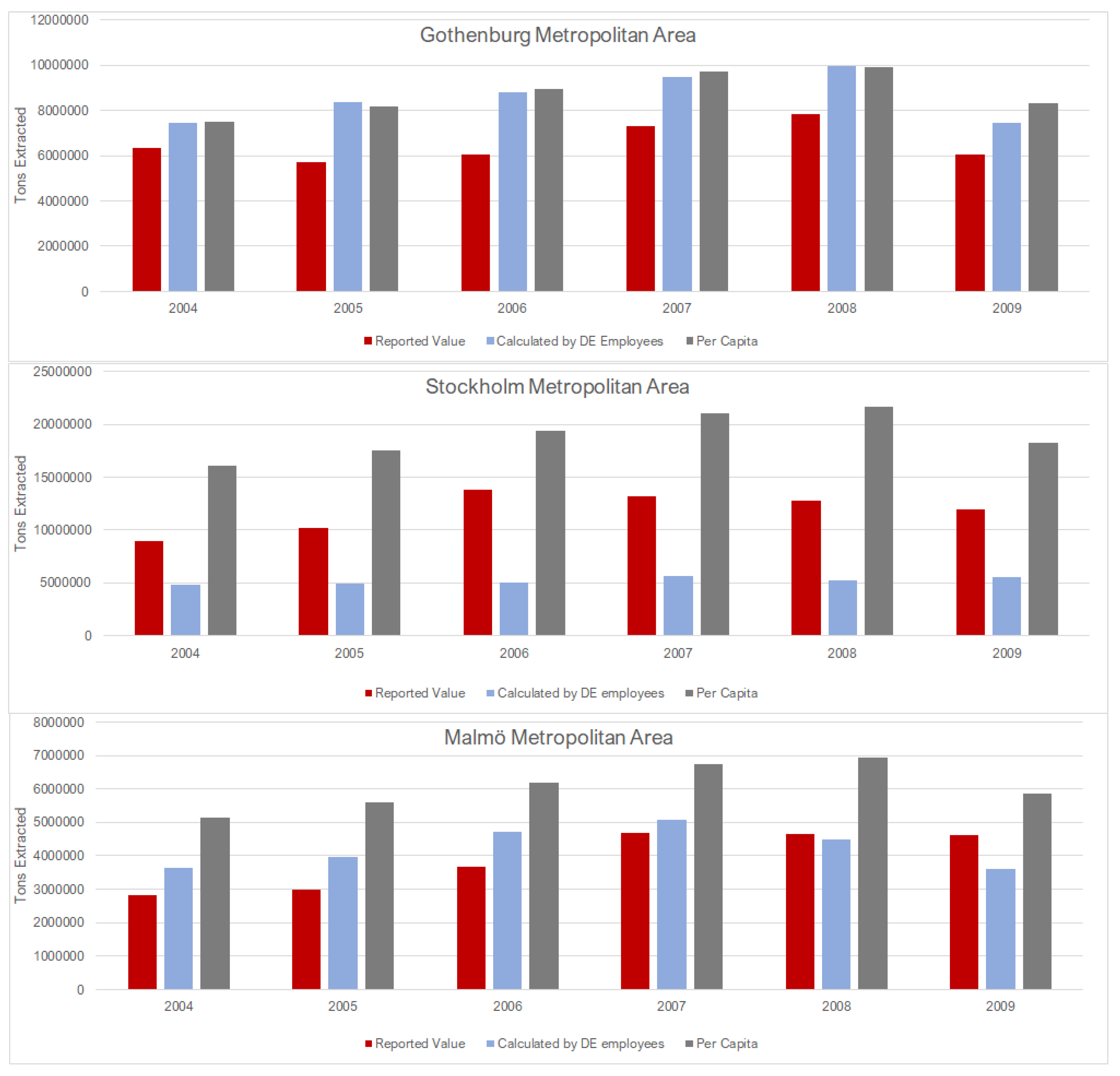
The purpose of this investigation was to search for proxies for more rigorous analysis that are sufficiently accurate to enable effective decision making. The evaluation of extrapolation methods began with a test to see how well the employee ratio method estimated extraction as a precursor to estimating consumption. The results indicated that using an economic sector’s employee ratio may estimate domestic extraction with reasonable accuracy at the county (NUTS3) level, giving a significantly more accurate estimate of true extraction than using per capita values. This was particularly true for Stockholm and Skåne counties, which may be due to the metabolism types of these regions. For example, Stockholm County houses the Stockholm Metropolitan Area, which has a service-based economy, and Skåne is responsible for most agriculture in Sweden. This indicates that per capita calculations would not be able to capture the difference in these areas. However, both the employee ratio method and the per capita calculation overestimated the metropolitan area DE for Gothenburg and Malmö metropolitan areas. This may be due to the fact that domestic extraction of aggregates tends to take place outside of metropolitan areas [33]. Stockholm Metropolitan Area aggregate consumption was underestimated by the employee ratio, which may indicate that there are employees working for companies registered in the surrounding area that are extracting materials within the metropolitan area instead.

Wine consumption was accurately estimated using the retail employee ratio at the county level. The results show, however, that the inclusion of wholesale employees would clearly lead to a significant misrepresentation of consumption values. Given that wholesale distributors are often located in one or a few locations [34], this would likely be the case for the majority of product types. Swedish employee data show that most employees working in wholesale NACE categories are centralized in one or a few regions.

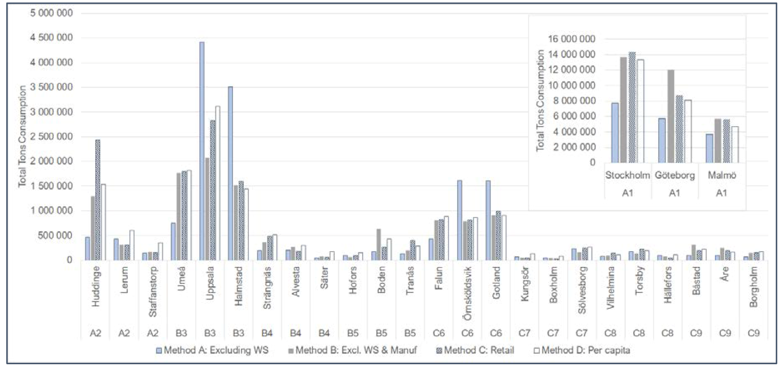
We can compare the total tons of consumption (all products) of Stockholm County (SE110), which is synonymous with the Stockholm Metropolitan Area, to the UMAn model results in Kalmykova et al. (2015b). Method A (all NACE codes except for wholesale) had similar results to the sum total (approximately 16 million tons using Method A, 19 million tons using the UMAn model), while Methods B (all NACE codes except wholesale and manufacturing), C (only retail NACE codes), and D (per capita) had significantly higher results (29 to 33 million tons total). The driver of the mass differences was primarily construction materials like wood (CN category 44) and stone (CN category 25). Product category CN25 is the heaviest of all CN2 categories and therefore can affect total tonnage results significantly. The differences in values for both CN25 and CN44 may be because they are both final and intermediate goods. In the UMAn results, category CN25 comprises approximately 50% of the total consumption mass, which is also true for Methods B, C, and D. Only Method A results in a smaller value than 50%, i.e., 34% of the total consumption mass. This further indicates that including manufacturing NACE codes (Method A) leads to inaccuracies. This also means that construction materials may therefore require additional analysis if measures requiring the use of these product types are to be considered. The majority of the remaining product categories are within the same percentage range as the UMAn model. Further details can be found in Supplementary Tables S3 and S4.

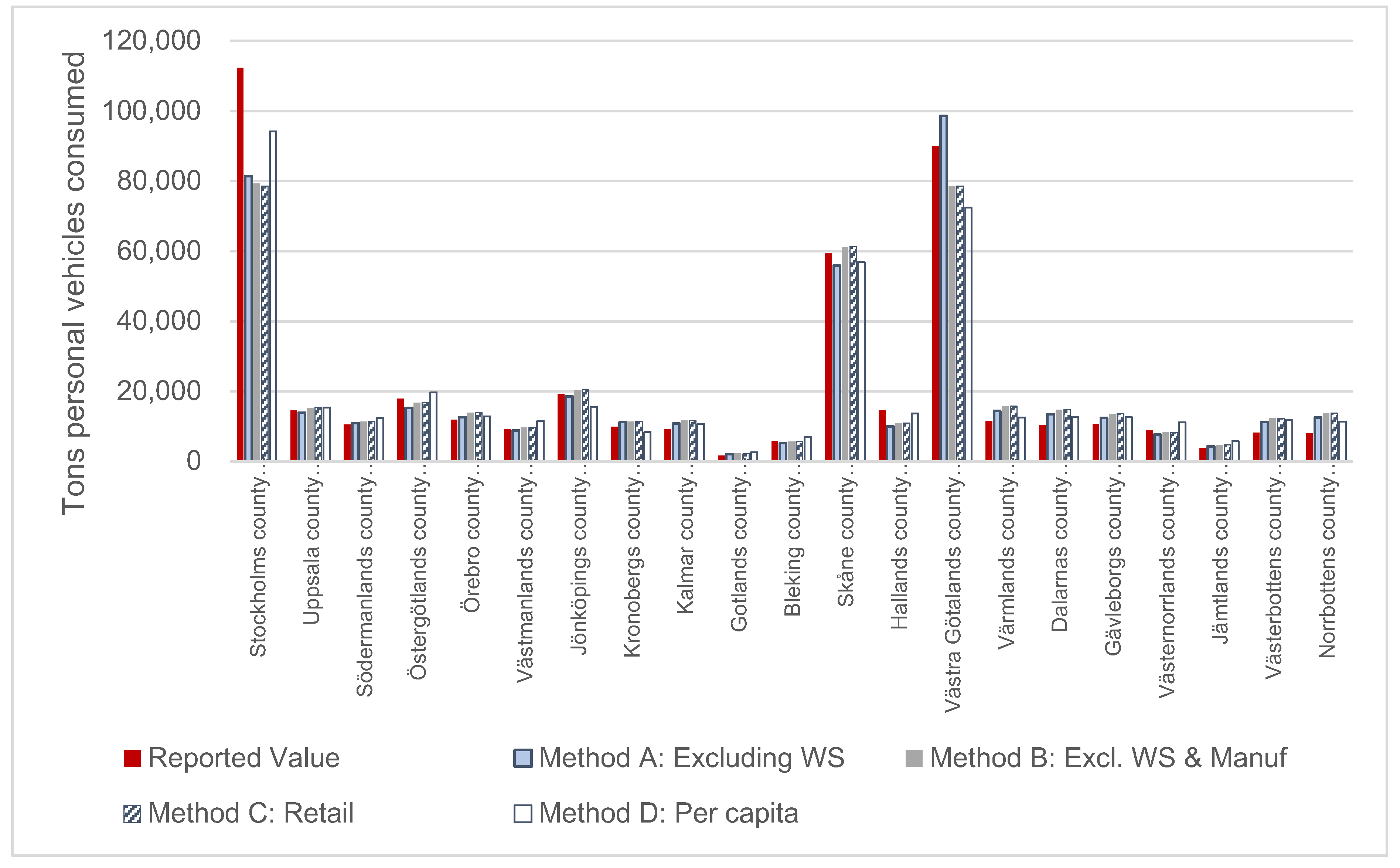
When comparing results to reported values at the county level, results using the employee ratio either did not match reported values as well as per capita estimates or had similar results to per capita results. Of the three novel extrapolation methods analyzed, Method A (all NACE codes excluding wholesale) had the most inaccurate results when compared to reported values at both the county and municipal levels and should therefore not be considered for future applications. At the county level, Methods B, C, and D led to similar results, with a 17% difference among them on average in vehicles and a 24% difference in fuel. The results indicate that at the county (NUTS3) level, per capita values are sufficient for final consumption extrapolation purposes.

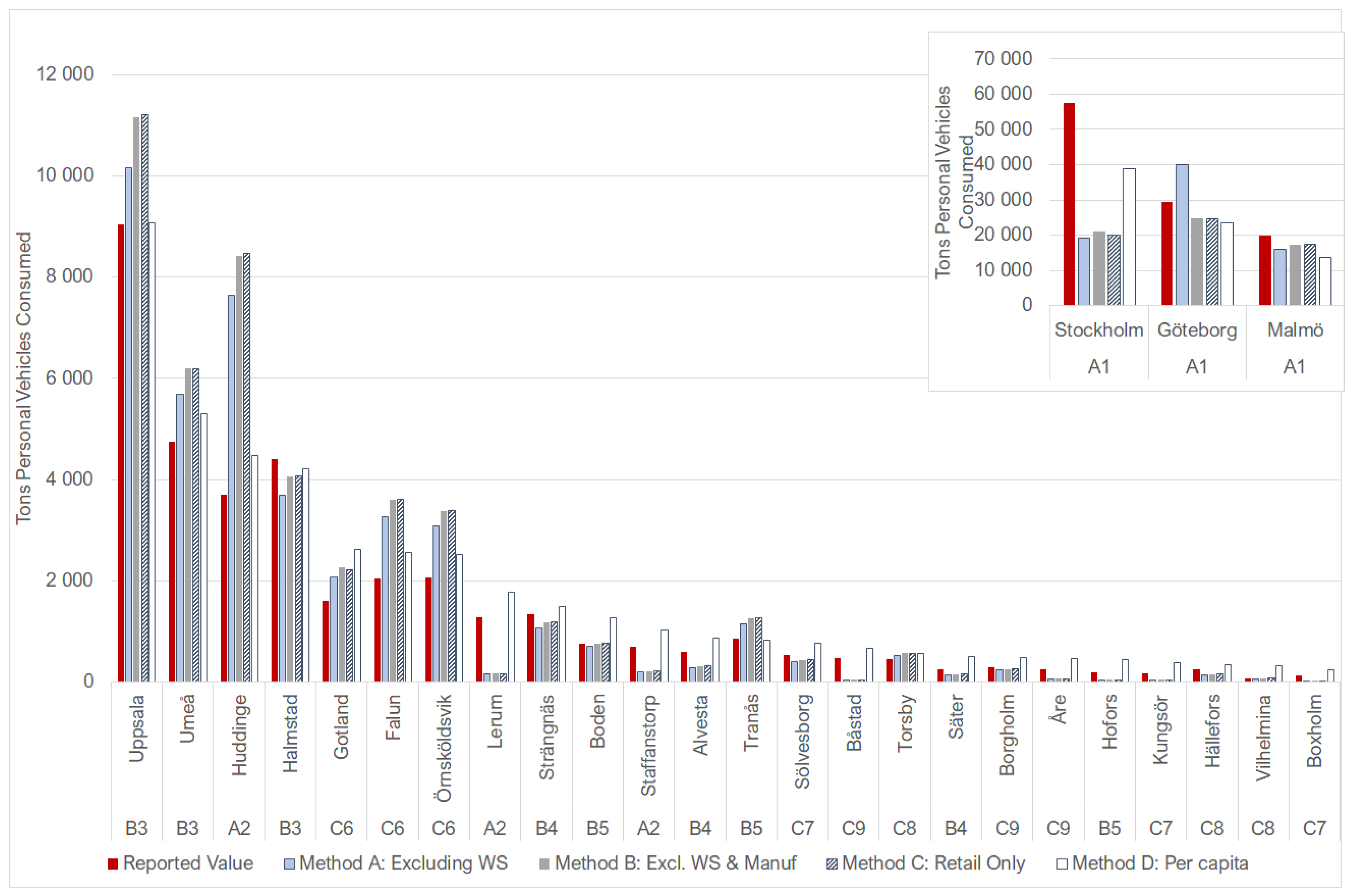
At the municipal level, the results for the employee ratio methods B and C were closer to reported values than per capita values on average but gave inaccurate results for those areas where employees for a certain NACE code were not present. For example, in small municipalities, there may not be any employees working in a particular sector (e.g., vehicle sales), and therefore consumption would be underestimated. The inaccuracies may be due to the fact that metropolitan areas and municipalities can be dependent on the hinterland; consumption in one area may actually be linked to extraction from a geographically distant area [35]. There was no clear correlation between municipality size and accuracy of results, although per capita values significantly overestimated vehicle consumption in municipalities smaller than 10,000 inhabitants. A link between population size and accuracy was not seen in the fuel results.

We found that using per capita values for final consumption was satisfactory for counties. This was also the case for municipalities with populations outside of major metropolitan areas with population sizes of up to 500,000. Method B (excluding wholesale and manufacturing economic sectors) gave considerably more accurate results than per capita values on average at the municipal level, but there was not a correlation between population size and accuracy. The level of accuracy needed will be dependent on the purpose of the extrapolation.

The method of evaluation presented in this article is limited by the number of products with reported values at the local level and could be improved by including more of these. Moving forward, we would like to gather bottom-up data on product consumption values (thus reducing the limitation to products with reported values) for the purposes of comparison and further evaluation of which method achieves the most reliable results. Testing the methods using other countries’ data would also improve the applicability and allow for greater generalizations.

References

1. United Nations Environment Programme; Fischer-Kowalski, M.; Swilling, M.; von Weizsäcker, E.U.; Ren, Y.; Moriguchi, Y.; Crane, W.; Krausmann, F.; Eisenmenger, N.; Giljum, S.; et al. Decoupling Natural Resource Use and Environmental Impacts from Economic Growth: A Report of the Working Group on Decoupling to the International Resource Panel; UNEP: Nairobi, Kenya, 2011; ISBN 9789280731675. [Google Scholar]
2. United Nations. Transforming Our World: The 2030 Agenda for Sustainable Development; United Nations: New York, NY, USA, 2015. [Google Scholar]
3. United Nations Goal 12: Sustainable Development Knowledge Platform. Available online: https://sustainabledevelopment.un.org/sdg12 (accessed on 2 July 2020).
4. Graute, U. Local Authorities Acting Globally for Sustainable Development. Reg. Stud. 2016, 50, 1931–1942. [Google Scholar] [CrossRef]
5. Bianchi, M.; Tapia, C.; Valle, I. Monitoring domestic material consumption at lower territorial levels A novel data downscaling method. J. Ind. Ecol. 2020, 1–14. [Google Scholar] [CrossRef]
6. Huysman, S.; Schaubroeck, T.; Goralczyk, M.; Schmidt, J.; Dewulf, J. Quantifying the environmental impacts of a European citizen through a macro-economic approach, a focus on climate change and resource consumption. J. Clean. Prod. 2016, 124. [Google Scholar] [CrossRef]
7. Miehe, R.; Scheumann, R.; Jones, C.M.; Kammen, D.M.; Finkbeiner, M. Regional carbon footprints of households: A German case study. Environ. Dev. Sustain. 2016, 18, 577–591. [Google Scholar] [CrossRef] [Green Version]
8. Druckman, A.; Jackson, T. The carbon footprint of UK households 1990–2004: A socio-economically disaggregated, quasi-multi-regional input-output model. Ecol. Econ. 2009, 68, 2066–2077. [Google Scholar] [CrossRef] [Green Version]
9. Thomas, B.A.; Azevedo, I.L. Estimating direct and indirect rebound effects for U.S. households with input-output analysis Part 1: Theoretical framework. Ecol. Econ. 2013, 86, 199–210. [Google Scholar] [CrossRef]
10. Whetstone, A.; Kalmykova, Y.; Rosado, L.; Westin, A.L. Informing sustainable consumption in urban districts: A method for transforming household expenditures into physical quantities. Sustainability 2020, 12, 802. [Google Scholar] [CrossRef] [Green Version]
11. Heinonen, J.; Junnila, S. A carbon consumption comparison of rural and urban lifestyles. Sustainability 2011, 3, 1234–1249. [Google Scholar] [CrossRef] [Green Version]
12. Collins, A.; Flynn, A.; Wiedmann, T.; Barrett, J. The environmental impacts of consumption at a subnational level: The ecological footprint of Cardiff. J. Ind. Ecol. 2006, 10, 9–24. [Google Scholar] [CrossRef]
13. Froemelt, A.; Buffat, R.; Heeren, N.; Hellweg, S. Assessing environmental impacts of individual households: A large-scale bottom-up LCA-model for Switzerland. In Proceedings of the SETAC Europe 28th Annual Meeting, Rome, Italy, 13–17 May 2018; pp. 32–33. [Google Scholar]
14. Roibás, L.; Loiseau, E.; Hospido, A. Determination of the carbon footprint of all Galician production and consumption activities: Lessons learnt and guidelines for policymakers. J. Environ. Manag. 2017, 198, 289–299. [Google Scholar] [CrossRef] [PubMed]
15. Froemelt, A. Data Mining Meets Life Cycle Assessment: Towards Understanding and Quantifying Environmental Impacts of Individual Households. Ph.D. Thesis, ETH Zurich, Zurich, Switzerland, 2018. [Google Scholar]
16. Minx, J.; Weidmann, T.; Wood, R.; Lenzen, M.; Peters, G.P.; Owen, A.; Scott, K.; Barrett, J.C.; Hubacek, K.; Baiocchi, G.; et al. Input-Output Analysis and Carbon Footprinting: An Overview of Applications. Econ. Syst. Res. 2009, 21, 187–216. [Google Scholar] [CrossRef]
17. Vita, G.; Lundström, J.R.; Hertwich, E.G.; Quist, J.; Ivanova, D.; Stadler, K.; Wood, R. The Environmental Impact of Green Consumption and Sufficiency Lifestyles Scenarios in Europe: Connecting Local Sustainability Visions to Global Consequences. Ecol. Econ. 2019. [Google Scholar] [CrossRef]
18. Larsen, H.N.; Hertwich, E.G. Identifying important characteristics of municipal carbon footprints. Ecol. Econ. 2010, 70, 60–66. [Google Scholar] [CrossRef]
19. Larsen, H.N.; Hertwich, E.G. The case for consumption-based accounting of greenhouse gas emissions to promote local climate action. Environ. Sci. Policy 2009, 12, 791–798. [Google Scholar] [CrossRef]
20. Kalmykova, Y.; Rosado, L.; Patrício, J. Resource consumption drivers and pathways to reduction: Economy, policy and lifestyle impact on material flows at the national and urban scale. J. Clean. Prod. 2015, 1–11. [Google Scholar] [CrossRef] [Green Version]
21. Rosado, L.; Kalmykova, Y.; Patrício, J. Urban metabolism profiles. An empirical analysis of the material flow characteristics of three metropolitan areas in Sweden. J. Clean. Prod. 2016, 126, 206–217. [Google Scholar] [CrossRef]
22. Lavers Westin, A.; Kalmykova, Y.; Rosado, L.; Oliveira, F.; Laurenti, R.; Rydberg, T. Combining material flow analysis with life cycle assessment to identify environmental hotspots of urban consumption. J. Clean. Prod. 2019, 226, 526–539. [Google Scholar] [CrossRef]
23. Eurostat Europa—RAMON—Classification. Available online: https://ec.europa.eu/eurostat/ramon/nomenclatures/index.cfm?TargetUrl=LST_CLS_DLD&StrNom=NACE_1_1 (accessed on 2 July 2020).
24. Commission, E. The Combined Nomenclature. Available online: http://ec.europa.eu/taxation_customs/customs/customs_duties/tariff_aspects/combined_nomenclature/index_en.htm (accessed on 12 April 2016).
25. Rosado, L.; Niza, S.; Ferrao, P. A Material Flow Accounting Case Study of the Lisbon Metropolitan Area using the Urban Metabolism Analyst Model. J. Ind. Ecol. 2014, 18, 84–101. [Google Scholar] [CrossRef]
26. Eurostat Principles and Characteristics. Available online: https://ec.europa.eu/eurostat/web/nuts/principles-and-characteristics (accessed on 2 July 2020).
27. Eurostat Glossary: Material Flow Indicators. Available online: https://ec.europa.eu/eurostat/statistics-explained/index.php/Glossary:Material_flow_indicators (accessed on 24 August 2020).
28. Martinez-Alier, J.; Muradian, R. (Eds.) Handbook of Ecological Economics; Edward Elgar Publishing: Cheltenham, UK, 2015; ISBN 9781783471409. [Google Scholar]
29. Statistics Sweden Nyregistrerade Personbilar Efter Län och Kommun Samt Drivmedel. Månad 2006M01–2020M06. Available online: http://www.statistikdatabasen.scb.se/pxweb/sv/ssd/START__TK__TK1001__TK1001A/PersBilarDrivMedel/ (accessed on 2 July 2020).
30. Trafikanalys. Trafikanalys Statistik över Fordonsflottans Utveckling—Delredovisning av Regeringsuppdrag; Trafikanalys: Stockholm, Sweden, 2016. [Google Scholar]
31. Kalmykova, Y.; Rosado, L.; Patrício, J. Urban Economies Resource Productivity and Decoupling: Metabolism Trends of 1996–2011 in Sweden, Stockholm, and Gothenburg. Environ. Sci. Technol. 2015, 49, 8815–8823. [Google Scholar] [CrossRef] [PubMed]
32. Swedish Association of Local Authorities and Regions. Classification of Swedish Municipalities.2017. Available online: https://skr.se/download/18.6b78741215a632d39cbcc85/1487772640274/ClassificationofSwedishMunicipalities2017.pdf (accessed on 2 July 2020).
33. Geological Survey of Sweden. Grus, Sand Och Krossberg 2016 (Aggregates); Elanders Sverige AB: Uppsala, Sweden, 2017. [Google Scholar]
34. Kjøtt-Larsen, T.; Schary, P.B.; Mikkola, J.H.; Kotzab, H. Distribution. In Managing Global Supply Chains; Copenhagen Business School Press: Copenhagen, Denmark, 2007. [Google Scholar]
35. Lenzen, M.; Peters, G.M. How City Dwellers Affect Their Resource Hinterland. J. Ind. Ecol. 2010, 14, 73–90. [Google Scholar] [CrossRef]
Figure 1. Overview of methods evaluated.
Sustainability 12 08336 g001
Figure 2. The sum of tons of wheat, rye, barley, and oats extracted by county per year compared to calculated extraction based on number of employees and using per capita values. Reported values are shown in red.
Sustainability 12 08336 g002
Figure 3. The sum of tons of aggregates extracted by metropolitan area per year compared to calculated extraction based on number of employees and using per capita values. Reported values are shown in red.
Sustainability 12 08336 g003
Figure 4. Wine consumption by county based on reported values, calculated using employees in retail, per capita, and wholesale. Reported values are shown in red.
Sustainability 12 08336 g004
Figure 5. Total consumption (tons) of all goods by county in 2010 using the four extrapolation methods.
Sustainability 12 08336 g005
Figure 6. Total consumption (tons) by municipality in 2010 using the four extrapolation methods.
Sustainability 12 08336 g006
Figure 7. Tons of new personal vehicles consumed by county in 2010 based on the different extrapolation methods used compared to the reported value. Reported values are shown in red.
Sustainability 12 08336 g007
Figure 8. Tons of new personal vehicles consumed by municipality in 2010 based on the different extrapolation methods used compared to the reported value. The three largest municipalities can be seen in the inset; the remaining municipalities are presented in order of decreasing size. Reported values are shown in red.
Sustainability 12 08336 g008