Article

The Intensity Analysis of Production Living Ecological Land in Shandong Province, China

1
School of Geography and Tourism, Qufu Normal University, Rizhao 276800, China
2
National Ecosystem Science Data Center, Key Laboratory of Ecosystem Network Observation and Modeling, Institute of Geographic Sciences and Natural Resources Research, Chinese Academy of Sciences, Beijing 100101, China
*
Author to whom correspondence should be addressed.
Sustainability 2020, 12(20), 8326; https://doi.org/10.3390/su12208326
Submission received: 14 September 2020 / Revised: 2 October 2020 / Accepted: 3 October 2020 / Published: 10 October 2020

Abstract

:
Due to the limitedness of land, the coordinated development of production, living, and ecological (PLE) land is essential for sustainable development. A clear understanding of PLE land change is necessary given the increased human activities, especially in developing regions. This study first reclassified remotely sensed landuse maps in Shandong province into PLE land. Then the spatiotemporal change of PLE land between 2000 and 2015 was analyzed using spatial trajectory and intensity analysis methods. The results show that the rate of PLE land change in the interval of 2000–2005 was the highest, and it kept decreasing during 2005–2010 and 2010–2015. The overall quantity component accounts for more difference than the exchange and shift components for all intervals. At the category level, the largest quantity component of change was PE land loss, followed by LP land gain. LP land gain targeted PE land intensively in each interval. The loss of E land was mainly to PE land in terms of size, and to PL land in terms of intensity. The findings of this study contribute to a deeper understanding of the spatiotemporal transitions of PLE land in Shandong province, which could help policy making for PLE land regulation.

1. Introduction

Given current economic development and rapid urbanization and their effects on the ecological environment, the balance of land multi-function has attracted increasing attention from scholars, planners, and policy makers [1]. How Production, Living, and Ecological land (PLE) is being spatiotemporally adjusted in the process of urbanization deserves to be studied. Optimizing PLE land has become an important principle in spatial planning and sustainable development strategy drafting [2]. However, many previous studies focused on the spatiotemporal change of remotely-sensed land-use types [3], with inadequate analysis on the change of multifunction-based land patterns. A comprehensive investigation on PLE land transition is more necessary than ever.
PLE land was emphasized in the report of the 18th National Congress of the Communist Party of China in 2012 for promoting the coordinated and sustainable development of economy and ecology [4]. Land can provide a variety of products and services for humans. Collectively, the production function refers to ability of providing agricultural, forestry and industrial products. The living function refers to the role of human habitation and survival. The ecological function is the capacity to improve the ecological environment and guarantee ecology security. In the past, people paid more attention to the production and living function of land. However, the ecological function is also very important for rational and sustainable utilization of land. Recently, studies on PLE land have increased. There are some studies on the PLE function calculation [5,6], PLE classification system [7,8,9,10], development status [4], eco-environment effects [11], and so forth. With regard to the PLE land classification, some studies proposed conceptual frameworks. Zhang et al. developed a practical PLE classification system based on land functions, which could be applied to reclassify the remotely sensed land use and land cover data into PLE land data [8]. The PLE land change processes could provide important implications for the sustainable management of land resources and for alleviating PLE space conflicts [2]. Given the impacts of PLE land change on environment, food safety, and economy, it is crucial to analyze the evolution characteristics of PLE land. However, a detailed quantitative analysis of the spatiotemporal changes of PLE land is limited in current research.
Although the quantitative assessment and spatial characteristics analysis of remotely sensed land use change were previously performed at different spatiotemporal scales, there is a lack of research on PLE land change processes. The spatiotemporal changes of PLE land can be investigated by commonly used methods, such as the transfer matrix [12], dynamic degree model [13,14,15], change trajectory or Geo-information Tupu analysis [16,17], intensity analysis [18,19,20], and some other complex algorithms [13]. Transfer matrix is a two-dimensional table of numbers, which is usually used as the basis for further analysis. The matrix’s rows are the categories at the start time point, and the columns are the categories at the end time point. The numbers on the matrix’s diagonal are the sizes of persistence of the category, and the numbers off the diagonal indicate the quantity of transfer from one category to another. The trajectory analysis can trace the categorical change of each pixel in the study region, which can result in a raster map showing the conversions between categories. Dynamic degree model calculates the temporal change rate of a specific category by dividing the annual net change size by the initial size of the category and the number of years. It can also measure the comprehensive dynamic degree by adding up the loss intensities of categories [14]. Intensity analysis is a framework, which reveals the difference of category changes during time intervals. The change scale, speed, change component for each category, and transition intensities among categories in different time intervals can be identified.
The most common application of intensity analysis is to investigate the land use change through time [21,22,23,24,25,26,27,28,29,30]. It can also be used to analyze other categorical research subjects. For example, Na et al. [31] used intensity analysis to quantify the dynamics of desertification. They analyzed the distribution of four aeolian desertified land levels in Hulunbuir during the 1980–2015 periods, thereby showing the change intensity of each level in different intervals. In the research field of drought variability, intensity analysis has been shown to be an effective tool [32,33,34]. The spatiotemporal variation characteristics of drought conditions were investigated using an intensity analysis approach. Moreover, intensity analysis was used to investigate the change of fractional vegetation coverage level from 1982 in Inner Mongolia quantitatively [35], and thereby found answers for the following questions: Is the annual change of vegetation coverage low or fast? Are the change of vegetation coverage dormant or active? What are the transition laws of different vegetation coverage degrees? With regard to the production, living, and ecological land, the intensity analysis has the potential to be an invaluable method for promoting in better understanding the change processes and possible causes.
Shandong province plays an important role in China’s national social and economic development [36]. It is one of China’s biggest agricultural production provinces. The urbanization rate increased from 39.2% in 2001 to 59.01% in 2015 [37,38]. A large area of high-quality cropland has been occupied by built-up land, and this trend may continue in the future [39]. Economic development has posed challenges to the ecological environment. The investigation of PLE land dynamics can provide fundamental data for research on sustainable development. However, the process of historical PLE land change of Shandong province has hitherto received limited attention. The main objective of this study is to demonstrate historical PLE land dynamics and transitions in Shandong province. Specifically, this study aims to: (1) classify and map the PLE categories at the time points 2000, 2005, 2010, and 2015, (2) determine the spatiotemporal trajectories of PLE land, and (3) analyze the types and processes of PLE land changes. The results of this study are useful for a better identification of PLE land change and for sustainable land resource management.

2. Materials and Methods

2.1. Study Area

Shandong province is located in the eastern part of China (114°19′–122°43′ E, 34°22′–38°15′ N) (Figure 1). It features a warm-temperate continental monsoon climate. The annual mean temperature is 11–14 °C, and the annual precipitation is 55–95 cm. It is one of the major agricultural regions in China. The proportion of cropland area in Shandong is 65%, and it plays an important role in food provision in China. The economic growth of Shandong province is also outstanding. The gross domestic product was 7.65 trillion RMB in 2018, which was nine times higher than in 2000. The population was 89.98 million in 2000 and 100.47 million in 2018. Along with the development of the economy and the growing of the population, the land use change was remarkable [40]. The built-up land area increased from 20,339 km2 to 23,989 km2 during 2000 and 2018.

2.2. Data

The land use data for 2000, 2005, 2010, and 2015, with 30 m × 30 m spatial resolution, were obtained from the Resource and Environment Data Cloud Platform [41]. The dataset was produced by the Chinese Academy of Sciences (CAS) based mainly on the Landsat TM/ETM+/OLI and GF-2 data using the human-machine interactive method. More details of the interpretation technology were presented in a previous study [42]. The interpretation results were validated against extensive field surveys, and the average classification accuracy was higher than 90% [43]. The land use types include 6 primary classes and 25 secondary classes. For example, the cropland includes paddy and non-irrigated uplands. The forest type includes high density forest, low density forest, shrub land, and orchards. The grassland includes high-, medium-, and low- density grassland. The water area includes rivers, canals, lakes, permanent glaciers, etc. The built-up land includes urban, rural settlements, and industrial land. The unused land includes desert, Gobi, wetland, bare land, rock, etc. This land use dataset has been widely used in land use change related research at the national and local levels [3,43].

2.3. Methods

2.3.1. Classification of Production-Living-Ecological Land

Some land use types often serve multiple functions [6]. For example, beyond the primary function of food production, cropland can also provide ecological benefits [44]. Urban area serves both the function of human living and production. Each land use type has a primary and secondary function. Zhang et al. (2017) put forward a Production Living Ecological land classification system for China, which consists of four categories: productive ecological land (PE), ecological productive land (EP), Living productive land (LP), and ecological land (E) [8]. The PE land includes cropland and orchard, which have important production functions, but also have some ecological functions. The EP land includes pasture, timberland, and aquaculture area. The LP land includes urban built-up and rural settlement. The E land includes ecological regulate regions, such as forest and grassland where are non-timber and non-pasture, and ecological conservation regions that are conserved as unused land.
In this study, we adopted the classification system of Zhang et al. [8]. We also made some modifications according to the local land use characteristics of the study area. We added the productive living land (PL) in this study. The reason is that the proportion of industrial built-up land in Shandong province is much larger than that within the national scale. The primary function of the industrial land is production, and they also serve the function of human living. Therefore, we classified the industrial built-up land as PL type, which are included in LP land in the classification system of Zhang et al. [8]. As a result, we reclassified the land use data of Shandong province into five function types: PE, EP, LP, PL, and E land based on the classification principle mentioned above. Then the spatiotemporal analysis on the PLE land between 2000 and 2015 was performed to describe PLE land succession on a pixel-by-pixel basis.

2.3.2. Intensity Analysis

Intensity analysis is a method of comparing maps with the same categories, spatial extent, and resolution [18,19,20]. For example, it could be used to analyze the land use maps at different time points and shows the size and intensity of land use change at the interval, category, and transition levels. Similarly, the spatiotemporal changes of PLE land between 2000 and 2015 were measured using the intensity analysis method in this study.
Intensity analysis quantifies the changes of size and intensity at increasingly detailed levels. Firstly, the interval level measures the total scale and speed of change in different time intervals. Equations (1) and (2) are as follows:
S t = { j = 1 J [ ( i = 1 J C t i j ) C t j j ] } / [ j = 1 J i = 1 J C t i j ] Y t + 1 Y t
where St is the annual change rate during the period [Yt,Yt+1]; Yt is the year at time point t. Subscripts i and j denote the categories, and the total number of categories is J, which is five in this study (PE, EP, PL, LP, and E land). Ctij is the area that changes from category i in year Yt to j in year Yt+1.
U = t = 1 T 1 { j = 1 J [ ( i = 1 J C t i j ) C t j j ] } / [ j = 1 J i = 1 J C t i j ] Y T Y 1
where U is the uniform value, which is the mean change rate. T is the number of time points, which is four in this study (2000, 2005, 2010, and 2015). If St is less than U, then the change rate of that period is relatively slow. Likewise, if St is larger than U, then the change rate of that period is relatively fast.
Furthermore, the overall change could be separated into three components, which are quantity, interval, and shift [19,20]. Quantity difference is the total amount of change between maps of different time points (Figure 2a); exchange is the spatial allocation difference that pairwise transitions cause (Figure 2b); shift is the spatial allocation difference that non-pairwise transitions cause (Figure 2c). The equations to compute these three components are presented in Pontius et al. [19,20].
The second level is category level, which produces the change trends for each individual category. For each period, the annual gain and loss of each category are calculated by Equations (3) and (4):
G a i n t j = [ ( i = 1 J C t i j ) C t j j ] / ( Y t + 1 Y t ) i = 1 J C t i j
L o s s t i = [ ( j = 1 J C t i j ) C t i i ] / ( Y t + 1 Y t ) i = 1 J C t i j
where Gaintj is annual gross gain intensity of category j and Lossti is annual loss intensity of category i for the period [Yt, Yt+1]. St computed by Equation (1) is the uniform intensity for each period. If the Gaintj or Lossti is less than St, then the change of category j or i during that period is dormant. On the contrary, if the Gaintj or Lossti is larger than St, then the change of category j or i is active. For the time interval t, the gross change of category j and its three components are computed by Equations (5)–(8) [45].
C h a n g e t j = G a i n t j + L o s s t j
Q u a n t i t y t j = | G a i n t j L o s s t j |
E x c h a n g e t j = 2 { [ i = 1 J M i n ( C t i j , C t j i ) ] C t j j }
S h i f t t j = C h a n g e t j Q u a n t i t y t j E x c h a n g e t j
where Changetj is gross change of category j for the time interval t. Changetj includes three components, which are the quantity component Quantitytj and the allocation components Exchangetj and Shifttj.
The third level is transition level, which measures the size and intensity that a category gains from other categories during a certain time interval. The intensities of transition to category n from each category i (in) are calculated using Equation (9):
R t i n = C t i n / ( Y t + 1 Y t ) j = 1 J C t i j
where Ctin is the area that changes from category i in the year Yt to category n in the year Yt+1. Equation (9) thus gives J − 1 transition intensities each period. The uniform transition intensity from other categories to category n during each period (Wtn) is computed using Equation (10).
W t n = [ ( i = 1 J C t i n ) C t n n ] / ( Y t + 1 Y t ) j = 1 J [ ( i = 1 J C t i j ) C t n j ]
Then if Rtin is less than Wtn, the gain of category n avoids j during the certain interval. Alternatively, if Rtin is larger than Wtn, the gain of category n targets j during that interval.

3. Results

3.1. Spatiotemporal Distributions of Prodution-Living-Ecological Land Changes

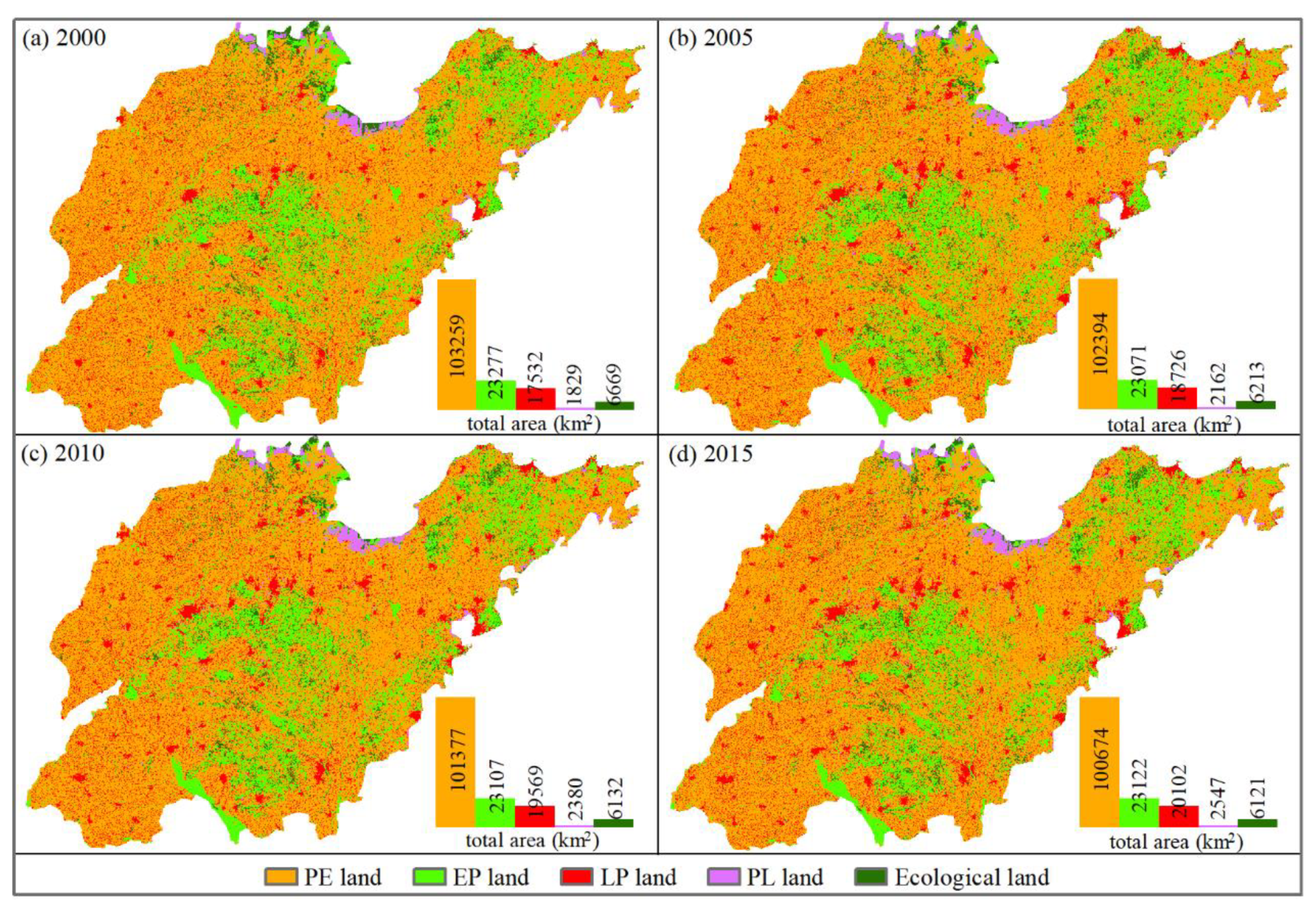
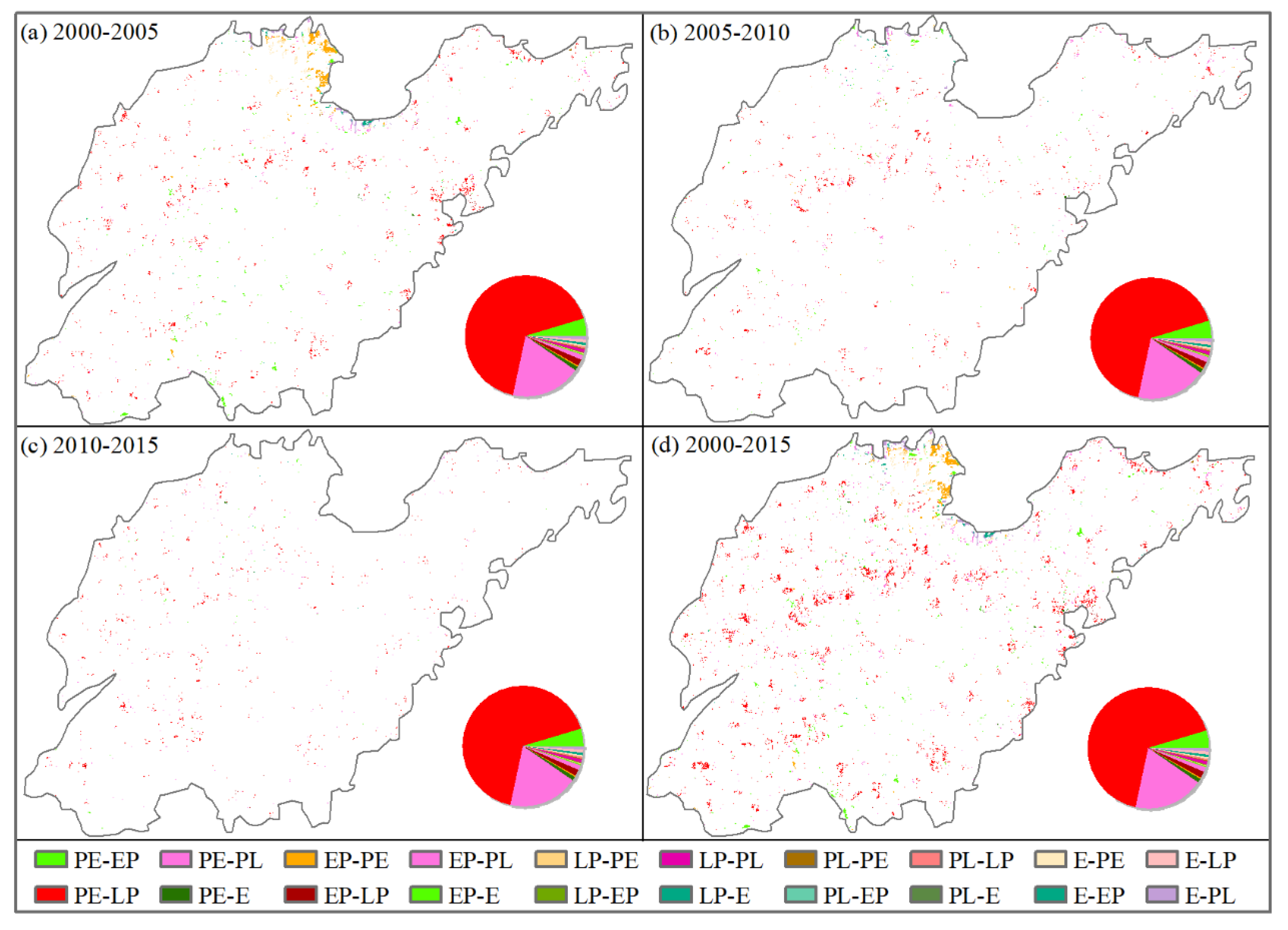
The spatial patterns of each category are shown Figure 3. The main type in the study area is PE land, which was 67.7% of the total area in 2000. The production function of PE land here is agricultural provision. The EP and E lands are mainly located in the upland area. Over the period from 2000 to 2015, the expansion of LP land was remarkable. The area of LP land increased rapidly from 17,532 km2 to 20,102 km2. Most of the newly expanded LP land was in the neighborhood of the original LP land. Due to the expansion of LP land, other categories were encroached by it to varying extents. A large proportion of the expansion of LP land was taking place in the PE land (Figure 4). Consequently, PE land suffered the largest decrease size. The reason for this may be because the PL lands and the PE lands are frequently located in proximity to each other.

3.2. Intensity Analysis of Prodution-Living-Ecological Land Change

3.2.1. Interval Level

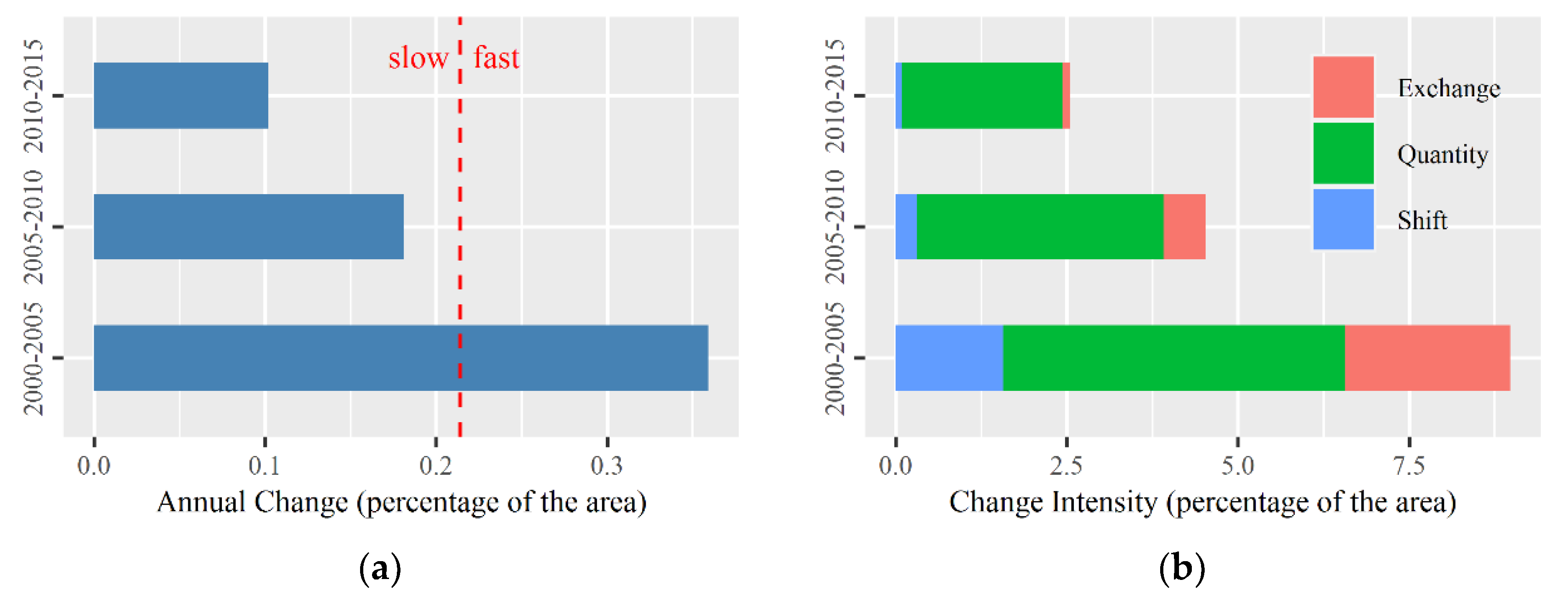
The results of interval level intensity analysis are shown in Figure 5a. The annual PLE land change percentage was the fastest during 2000 and 2005, followed by the period between 2005 and 2010. The PLE land change during 2010 and 2015 was the slowest. The red vertical dashed line in Figure 5a represents the uniform intensity value, which was calculated using Equation (2), and it was the mean change rate of the three time intervals. Furthermore, the overall annual change of each time interval was divided into three components: quantity, exchange, and shift (Figure 5b). The exchange and shift are two components of allocation difference, where exchange is the allocation difference that caused by pairwise transitions, and shift is the allocation difference caused by non-pairwise transition (Figure 2). The quantity component accounted for more difference than allocation components (exchange and shift) for all the three periods. Exchange was larger than shift during all the three periods.

3.2.2. Category Level

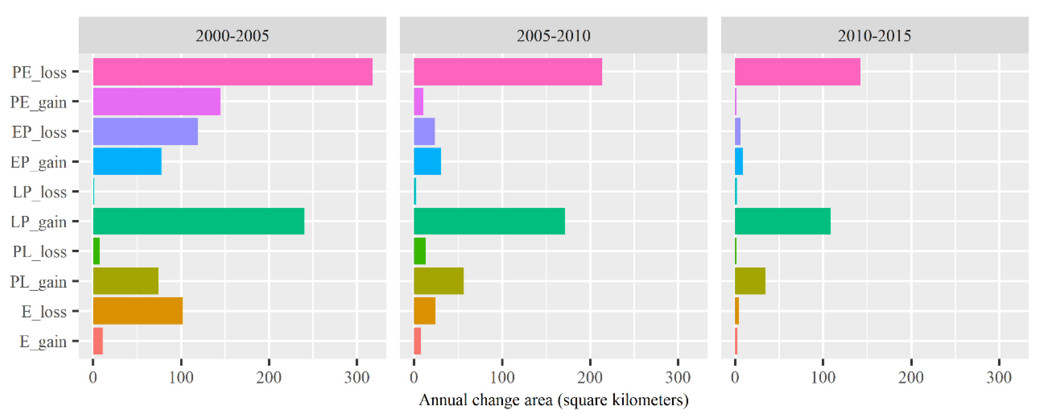
The areas of the annual gain or loss of each category during the three periods are revealed in Figure 6. The net change of each category was also derived. The PE land had the largest loss, and LP land had the largest gain during all of the three time intervals. The gain size of PL land was also relatively large. The loss in size of E land was big during the first time interval, then decreased obviously during the middle and the latter interval. The LP land loss sizes were small across the three periods. The sizes of gain and loss of all the categories were largest during the period 2000–2005, and were the smallest during the period 2010–2015.
In addition, change intensity of each category in terms of change per area of the category is shown in Figure 7. The red dashed line indicates the uniform change intensity calculated by Equation (2) for each period. If a bar ends beyond the uniform intensity line, then the change is active. On the contrary, if a bar ends before the uniform intensity line, then the change is dormant. The gains of LP and PL land were active during all of the three time intervals. Although the size of PE land loss was the largest (Figure 6), the loss of PE land was dormant (Figure 7). PE land’s large size in the denominator of its intensity led the intensity of PE land loss to be dormant. Accordingly, PE land’s large size was responsible for its large losses. E land’s loss intensities were active during the periods 2000–2005 and 2005–2010, but turned to dormant in the interval of 2010–2015.
EP and PE land were mainly responsible for the exchange component, especially during 2000 and 2005 (Figure 8a). A closer look at the processes revealed that the PE land includes cropland and orchard, and PE land includes pasture and timberland; therefore, a large part of allocation changed during the former two periods, involving the transition from cropland and orchard to pasture and timberland, and from pasture and timberland to cropland and orchard. The sign of net loss and net gain associated with each category denoted the loss and gain of the quantity component during each interval, respectively. LP and PE land were mainly responsible for the quantity change component during all the three time intervals, while LP and PL land were net gaining categories, and PE, EP, and E land were net losing categories. The process was an expansion of LP land (such as urban area) in the study area, where usually the available land was PE (such as cropland) and E land.
The sizes of quantity, exchange, and shift components by category are challenging to compare due to the different size of each category. Therefore, the component intensity, which is the size of the component divided by the total size of the difference, can address this challenge. The component intensity for each category during the three periods are shown in Figure 8b. The vertical red dashed line represents the intensity of quantity component overall, which is the size of overall quantity component divided by the size of the three difference components (quantity, exchange, and shift) overall. The overall quantity components were 56%, 79%, and 92% of the difference overall during 2000–2005, 2005–2010, and 2010–2015 intervals respectively. Take the period 2000–2005 as an example. The quantity of PE and EP land ended before the quantity overall line, thus these two categories had less intensive quantity components compared with the overall quantity component. The quantity for LP, PL, and E land ended beyond the quantity overall line, and these three categories had more intensive quantity components compared with the overall quantity component. The blue vertical dashed line represents the sum of the intensities of quantity and exchange components overall, which are 83%, 93%, and 96% for the time intervals 2000–2005, 2005–2010, and 2010–2015 respectively. For each time interval, the difference between the red and the blue dashed line indicates the intensity of the overall exchange component. Take the time interval of 2000–2005 as an example, the blue dashed line of 83% indicates that the intensity of overall shift component is 17%. The shift intensity was just to the right of the blue dashed line. Therefore, during 2000 and 2005, PE land had a more intensive shift component compared with the shift component overall, while the other four categories had less intensive shifts compared with the shift component overall.

3.2.3. Transition Level

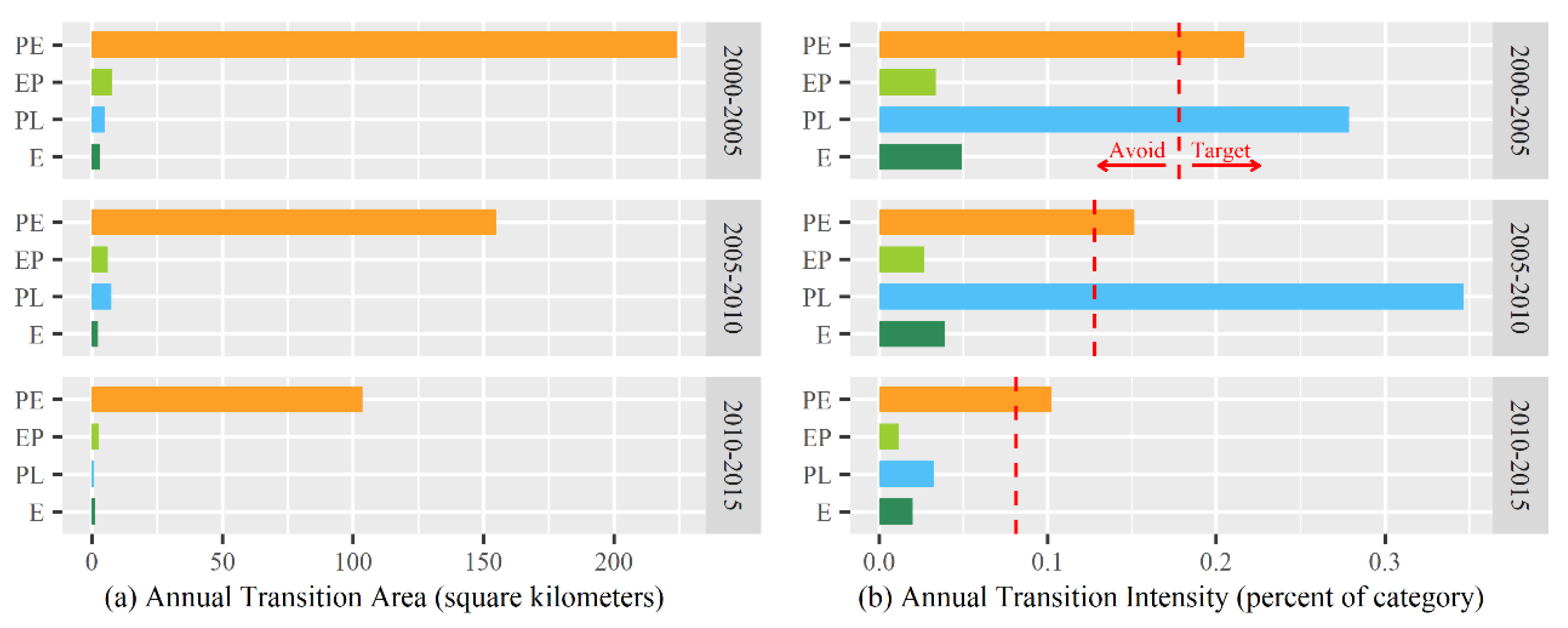
The quantity changes of PE land during the three intervals were net loss. The annual loss amount of PE land is revealed in Figure 9a, while the intensities for the categories to which PE land loses are revealed by Figure 9b. LP land had the largest transition size, followed by PL land. The transition intensity to PL was larger than to LP land, because PL accounted for a larger percentage of the study area than LP land. The red vertical dashed line in Figure 9b indicates the uniform change intensity for PE land loss, which was calculated using Equation (6). The bars of LP land and PL land ended beyond the uniform line. This reveals that when PE land was lost, it tended to lose intensively to LP and PL land more than other categories. That is to say, the loss of PE land targeted LP and PL land but avoided EP and E land during all the time intervals.
For the transition to PE land, the annual transition sizes and the intensities for the categories from which PE land gained are revealed in Figure 10. PE land gained most from EP and E land both in terms of the transition size and the intensity. The red vertical dashed line indicates the uniform change intensity of PE land gain during each period. If one category’s intensity bar ends before the uniform line, then the transition of this category avoids PE land. On the contrary, if a category’s intensity bar ends beyond the uniform line, then the transition of this category targets PE land. The transition intensities from E land to PE land extend to the right side of the uniform line in all of the three periods. There was a gain of PE land targeted EP land during the 2000–2005 and 2005–2010 period, but EP land was avoided during the interval of 2010–2015.
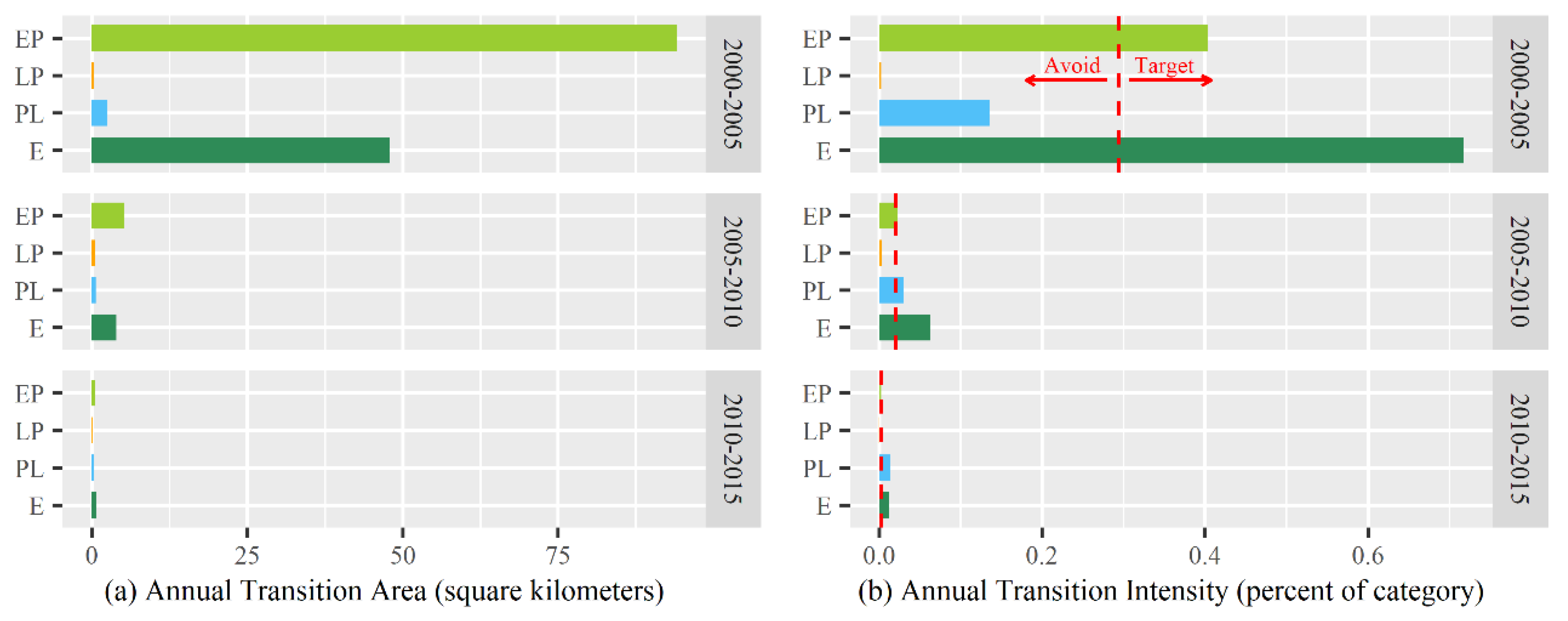
The quantity changes of PE land were net loss during the first interval, and net gain during the latter two intervals. The annual transition sizes and intensities for the categories from which EP land gains are shown in Figure 11. The red vertical dashed line indicates the uniform change intensity for the gain of EP land during each interval. If one category’s intensity bar ends on the left of the uniform line, then the transition of this category avoids EP land, and vice versa. The transition size from EP to PE land was largest during the first time interval. The transition intensity reveals that the loss of EP land was targeting PL and E land during all the intervals. The losses intensity of EP land to LP land was also larger than the uniform line during the latter two periods.
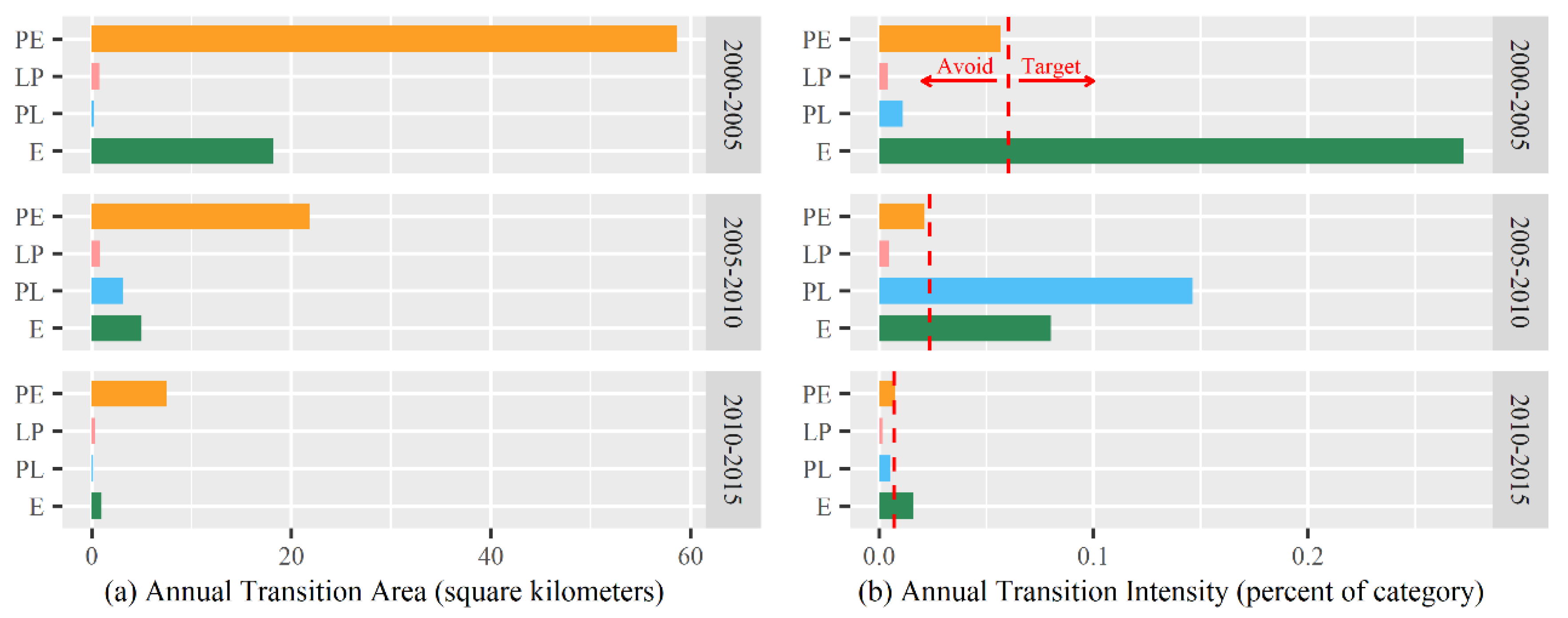
For transition to EP land, the annual transition sizes and intensities for the categories from which EP land gains are presented in Figure 12. The red vertical dashed line indicates the uniform change intensity for the gain of EP land during each interval. The transition sizes from PE to EP land are the largest during all of the three time intervals. However, the transition intensity reveals that the gain of EP land was avoiding PE land during all the intervals. Therefore, the large transition area from PE land to EP land could be attributed to the large percentage of PE land with the study area. The gain of EP land was targeting E land more than PE land in terms of transition intensity.
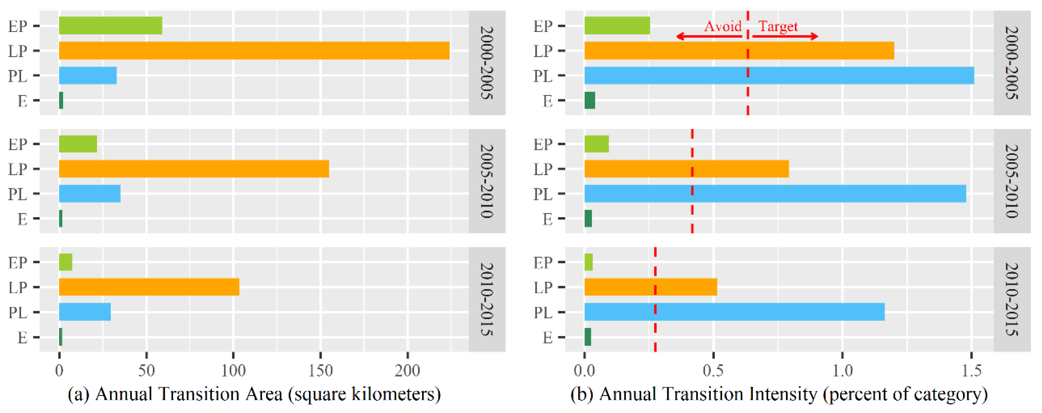
The interval level and categorical level analysis above show that the gain of LP land was largest both in terms of size and of intensity, followed by PL land. At the transition level, the annual transition size and the intensity for the categories from which LP land gained are shown in Figure 13. LP land gained first from PE land, and then from PL and EP land in terms of the annual transition area. However, the fact that the LP land gained more intensively from PL land than from PE land during the first two time intervals is revealed in Figure 13b. The reason is that the initial size of PE land was larger than PL land. Then the situation changed for the interval of 2010–2015, during which the bar for PL land was to the left of the uniform line. PE land was the only category that ended beyond the uniform line during all of the three time intervals.
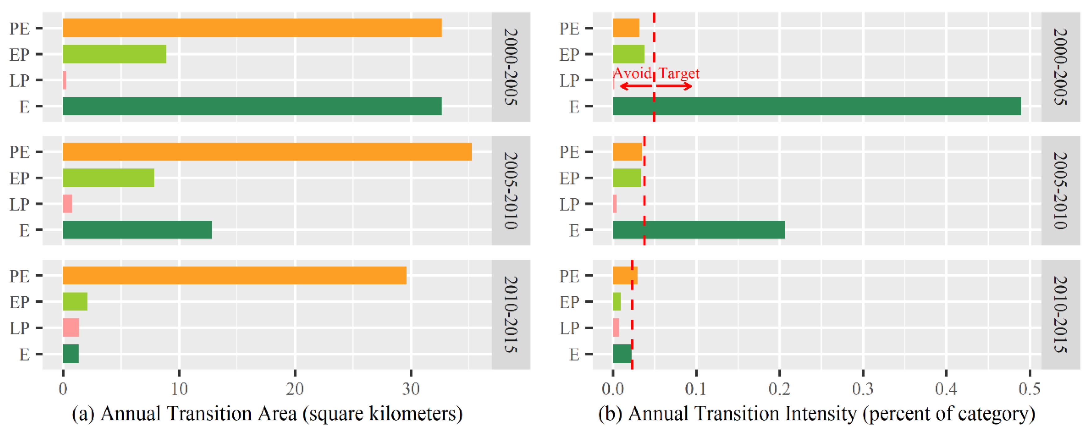
The results for the transitions to PL land are represented in Figure 14. PL land gained mainly from PE and E land in terms of annual transition size. However, the bar for PE land transition intensity extended before the uniform line, which revealed that PE’s start size was more crucial than PE’s transition intensity to account for the area of the transition. Both the transition size and the transition intensity of E land to PL land were large, except that the gain of PL land avoided E land during 2010 and 2015. The gain of PL targeted PE land during 2010–2015.
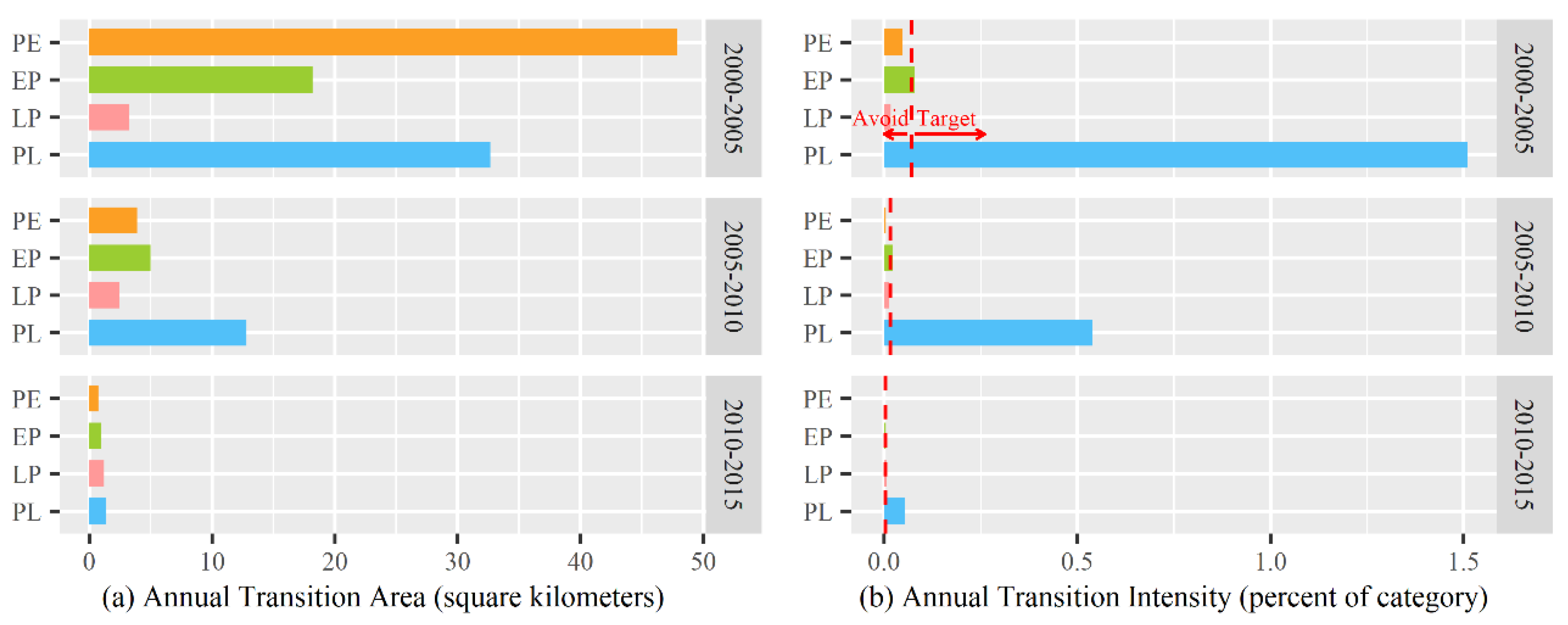
The quantity changes of E land were net loss during all the intervals. The results for the loss of E land are shown in Figure 15. The transition to PE land was much larger than to other categories during the first time interval. In terms of intensity, we see that the bar for EP and PL land extended to the right of the uniform line during all the intervals. Concerning the status of targeting and avoiding with regard to E land loss, all categories were stationary across the three periods.

4. Discussion

For all of the three time intervals, the largest quantity component of change among the five categories was for LP, which presented net gain. The second was for PE, which presented net loss. The further categorical results show that the largest gain of LP land was from PE land, and the largest loss of PE land was to LP land in terms of size, and to PL land in terms of intensity. The findings provide evidences to justify the concern of cropland loss because of explosive urban sprawl. The conversion of PE to LP and PL land was likely due to the urbanization, i.e., the transitions from cropland to urban area and industrial land, which were common in the study area.
Since 2000, the government had realized the issue of food insecurity due to the loss of cropland caused by rapid urbanization. The cropland protection policies were initiated due to concern for food security [46]. The cropland requisition-compensation balance policy requires a quantity balance between the losses in cropland that transfer to built-up land and the gains of cropland elsewhere [47]. In this study, we found that the gain of PE land was mainly from E land, and large size of E land transferred to PE land especially during the first interval. The potential negative effects of the cropland requisition-compensation balance policy on ecological environment deserve attention from the policymakers and public, especially in ecologically fragile regions. Meanwhile, the loss intensity from E land to PL land was the largest. This finding implies that the tradeoff and synergy between industrial production and ecosystem regulating and supporting services should be evaluated and considered in the land management.
The PLE land change was the fastest during 2000–2005; then, the change rate decreased in the latter two periods. The results suggest that the PLE land change rate in Shandong province decelerated steadily from 2000 to 2015. A few reasons for this are that the accumulation of negative effects on the environment, the measures the government has put forward to balance the positive effect on the economy, and the negative effect on food production have caused public concern. Land use policies and management including land consolidation, urban growth boundaries, and an ecological civilization program had been implemented to improve sustainability [48]. Another underlying reason is that the growth rate of GDP declined after 2010.
This study also has some limitations. First, there are some uncertainties in the PLE land classification system. The classification systems and the concepts for PLE land have not been unified until now. There are still some controversies in linking the PLE classification systems with the remotely sensed land cover classification systems. For example, the unused lands include the desert with vegetation cover lower than 5%, the saline and alkaline land, and bare rock, which are not suitable for production and living. Whether the unused lands should be included in the ecological land is indefinable. In this study, we classified unused lands as E land considering their ecological functions. Further research into the classification system of PLE land using scientific methods and techniques is needed. Second, the spatial resolution of the land use data used in this study is 30 × 30 m. The resolution is higher than many other studies of similar space scale. However, some typical ecological land was still ignored because their areas are relatively small. For example, some urban ecological land may be included in LP land, and some farm protection ecological land may be included in PE land, etc. To reduce error caused by mixed pixel, higher resolution land use data should be used. In this study, the study period is from 2000 to 2015. The reason is that the accuracy of the land use data before 2000 was too low to reveal the land use processes. In the future, more accurate land use data in 2020 and before 2000 would be derived using more advanced techniques. The time scale could then be refined.
This study investigated the historical PLE land changes; however, the projection of PLE land dynamics in the future is also a key issue for optimal allocation. A multitude of land use models have been developed for scenario projections, like CLUMondo [49], LandCA [50], LANDSCAPE [51], FLUS [52], and so forth. The next step would be to predict PLE land distribution under different scenarios based on land use dynamic models. The driving factors of PLE land change should also be analyzed quantitatively using statistical or machining learning methods in the future.

5. Conclusions

To sum up, this study presents a full picture of PLE land changes in Shandong province between 2000 and 2015. We first defined the PLE land classification system based on previous studies and the local characteristics of the study area. Then we assessed spatiotemporal change in PLE land by spatial trajectory analysis and intensity analysis. Overall, the results show that the PLE land, especially the PE and LP land, experienced notable changes during the studied period. In terms of the overall change level, the PLE land change was fastest during the first time interval 2000–2005, and was the slowest during 2010–2015. The quantity component is the largest among the three components during all intervals. At the categorical level, the size of PE land loss was the largest, followed by the gain of LP land. In terms of intensity, active transitions include the gains of LP and PL land during all intervals and the losses of E land during the first two intervals. The transition level results reveal that LP land’s gain targeted PE land during all intervals. The largest transition to PL was also from PE land. Large size of E land transferred to PE land during the first interval, and E land’s loss targeted PL land in all intervals. As noted above, policy making for PLE land coordination should be put forward. For example, the land use policies of the study area should take into account the protection of PE land. The appropriate restriction of LP land expansion would be helpful in preventing the conflicts with PLE land. Meanwhile, there should be concerted effort by government to supervise for effective enforcement of policies that protect E land from being occupied by PE land and PL land. It is essential to coordinate the PLE land for socioeconomic development, food provision, and ecological protection and abide by the rules of food security and ecology. The methods used in this research could be applied in the studies of other provinces or regions easily, however, it would be necessary to modify the PLE land classification principles according to the local conditions.

Author Contributions

Conceptualization, M.W. and J.W.; methodology, X.S. and C.Y.; software, X.S. and C.Y.; validation, M.W.; formal analysis, X.S.; investigation, X.S.; resources, M.W. and J.W.; data curation, X.S. and C.Y.; writing—original draft preparation, X.S.; visualization, X.S.; supervision, M.W.; funding acquisition, X.S. and J.W. All authors have read and agreed to the published version of the manuscript.

Funding

The Humanities and Social Sciences Foundation of the Ministry of Education in China (20YJCZH140), the National Key Research and Development Program of China (2016YFC0500203), the National Natural Science Foundations of China (31861143015).

Conflicts of Interest

The authors declare no conflict of interest.

References

  1. Martellozzo, F.; Amato, F.; Murgante, B.; Clarke, K.C. Modelling the impact of urban growth on agriculture and natural land in Italy to 2030. Appl. Geogr. 2018, 91, 156–167. [Google Scholar] [CrossRef] [Green Version]
  2. Lin, G.; Jiang, D.; Fu, J.; Cao, C.; Zhang, D. Spatial conflict of production-living-ecological space and sustainable-development scenario simulation in yangtze river delta agglomerations. Sustainability 2020, 12, 2175. [Google Scholar] [CrossRef] [Green Version]
  3. Hu, Y.; Batunacun; Zhen, L.; Zhuang, D. Assessment of land-use and land-cover change in Guangxi, China. Sci. Rep. 2019, 9. [Google Scholar] [CrossRef] [Green Version]
  4. Wang, D.; Jiang, D.; Fu, J.; Lin, G.; Zhang, J. Comprehensive assessment of production-living-ecological space based on the coupling coordination degree model. Sustainability 2020, 12, 2009. [Google Scholar] [CrossRef] [Green Version]
  5. Zou, L.; Liu, Y.; Yang, J.; Yang, S.; Wang, Y.; Cao, Z.; Hu, X. Quantitative identification and spatial analysis of land use ecological-production-living functions in rural areas on China’s Southeast Coast. Habitat Int. 2020, 100, 102182. [Google Scholar] [CrossRef]
  6. Yu, Z.; Xu, E.; Zhang, H.; Shang, E. Spatio-temporal coordination and conflict of production-living-ecology land functions in the Beijing-Tianjin-Hebei region, China. Land 2020, 9, 170. [Google Scholar] [CrossRef]
  7. Liao, G.; He, P.; Gao, X.; Deng, L.; Zhang, H.; Feng, N.; Zhou, W.; Deng, O. The production–living–ecological land classification system and its characteristics in the hilly area of Sichuan Province, Southwest China based on identification of the main functions. Sustainability 2019, 11, 1600. [Google Scholar] [CrossRef] [Green Version]
  8. Zhang, H.; Xu, E.; Zhu, H. Ecological-living-productive land classification system in China. J. Resour. Ecol. 2017, 8, 121–128. [Google Scholar]
  9. Liu, J.; Liu, Y.; Li, Y. Classification evaluation and spatial-temporal analysis of “production-living-ecological” spaces in China. Acta Geogr. Sin. 2017, 72, 1290–1304. [Google Scholar]
  10. Yang, X. Study on the “Ecological-Living-Productive” Land Classification System and Their Spatial Characteristics in Hebei Province. Master’s Thesis, Chang’an University, Xi’an, China, 2019. [Google Scholar]
  11. Yang, Q.; Duan, X.; Wang, L.; Jin, Z. Land use transformation based on ecological-production-living spaces and associated eco-environment effects: A case study in the Yangtze River Delta. Sci. Geogr. Sin. 2018, 38, 97–106. [Google Scholar]
  12. Foody, G.M. Status of land cover classification accuracy assessment. Remote Sens. Environ. 2002, 80, 185–201. [Google Scholar] [CrossRef]
  13. Huang, B.; Huang, J.; Pontius, R.G., Jr.; Tu, Z. Comparison of intensity Analysis and the land use dynamic degrees to measure land changes outside versus inside the coastal zone of Longhai, China. Ecol. Indic. 2018, 89, 336–347. [Google Scholar] [CrossRef]
  14. Quan, B.; Bai, Y.; Römkens, M.J.M.; Chang, K.-T.; Song, H.; Guo, T.; Lei, S. Urban land expansion in Quanzhou City, China, 1995–2010. Habitat Int. 2015, 48, 131–139. [Google Scholar] [CrossRef]
  15. Pontius, R.G.; Huang, J.; Jiang, W.; Khallaghi, S.; Lin, Y.; Liu, J.; Quan, B.; Ye, S. Rules to write mathematics to clarify metrics such as the land use dynamic degrees. Landsc. Ecol. 2017, 32, 2249–2260. [Google Scholar] [CrossRef]
  16. Lu, X.; Shi, Y.; Chen, C.; Yu, M. Monitoring cropland transition and its impact on ecosystem services value in developed regions of China: A case study of Jiangsu Province. Land Use Policy 2017, 69, 25–40. [Google Scholar] [CrossRef]
  17. Badjana, H.M.; Helmschrot, J.; Selsam, P.; Wala, K.; Fluegel, W.-A.; Afouda, A.; Akpagana, K. Land cover changes assessment using object-based image analysis in the Binah River watershed (Togo and Benin). Earth Space Sci. 2015, 2, 403–416. [Google Scholar] [CrossRef] [Green Version]
  18. Aldwaik, S.Z.; Pontius, R.G. Intensity analysis to unify measurements of size and stationarity of land changes by interval, category, and transition. Landsc. Urban Plan. 2012, 106, 103–114. [Google Scholar] [CrossRef]
  19. Pontius, R.G., Jr. Component intensities to relate difference by category with difference overall. Int. J. Appl. Earth Obs. Geoinf. 2019, 77, 94–99. [Google Scholar] [CrossRef]
  20. Pontius, R.G., Jr.; Santacruz, A. Quantity, exchange, and shift components of difference in a square contingency table. Int. J. Remote Sens. 2014, 35, 7543–7554. [Google Scholar] [CrossRef]
  21. Akodéwou, A.; Oszwald, J.; Saïdi, S.; Akpavi, S.; Akpagana, K.; Gond, V. Land use and land cover dynamics analysis of the togodo protected area and its surroundings in Southeastern Togo, West Africa. Sustainability 2020, 12, 5439. [Google Scholar] [CrossRef]
  22. Anteneh, Y.; Stellmacher, T.; Zeleke, G.; Mekuria, W.; Gebremariam, E. Dynamics of land change: Insights from a three-level intensity analysis of the Legedadie-Dire catchments, Ethiopia. Environ. Monit. Assess. 2018, 190. [Google Scholar] [CrossRef]
  23. Da, F.; Chen, X.; Qi, J. Spatiotemporal characteristic of land use/land cover changes in the middle and lower reaches of shule river basin based on an intensity analysis. Sustainability 2019, 11, 1360. [Google Scholar] [CrossRef] [Green Version]
  24. Ekumah, B.; Armah, F.A.; Afrifa, E.K.A.; Aheto, D.W.; Odoi, J.O.; Afitiri, A.-R. Assessing land use and land cover change in coastal urban wetlands of international importance in Ghana using Intensity Analysis. Wetl. Ecol. Manag. 2020, 28, 271–284. [Google Scholar] [CrossRef]
  25. Feng, Y.; Lei, Z.; Tong, X.; Gao, C.; Chen, S.; Wang, J.; Wang, S. Spatially-explicit modeling and intensity analysis of China’s land use change 2000–2050. J. Environ. Manag. 2020, 263. [Google Scholar] [CrossRef]
  26. Niya, A.K.; Huang, J.; Karimi, H.; Keshtkar, H.; Naimi, B. Use of Intensity Analysis to characterize land use/cover change in the biggest island of Persian Gulf, Qeshm Island, Iran. Sustainability 2019, 11, 4396. [Google Scholar] [CrossRef] [Green Version]
  27. Shoyama, K.; Braimoh, A.K.; Avtar, R.; Saito, O. Land transition and intensity analysis of cropland expansion in Northern Ghana. Environ. Manag. 2018, 62, 892–905. [Google Scholar] [CrossRef]
  28. Tankpa, V.; Wang, L.; Atanga, R.A.; Awotwi, A.; Guo, X. Evidence and impact of map error on land use and land cover dynamics in Ashi River watershed using intensity analysis. PLoS ONE 2020, 15. [Google Scholar] [CrossRef] [Green Version]
  29. Tong, S.; Bao, G.; Rong, A.; Huang, X.; Bao, Y.; Bao, Y. Comparison of the spatiotemporal dynamics of land use changes in four municipalities of China based on Intensity Analysis. Sustainability 2020, 12, 3687. [Google Scholar] [CrossRef]
  30. Zhao, Q.; Wen, Z.; Chen, S.; Ding, S.; Zhang, M. Quantifying land use/land cover and landscape pattern changes and impacts on ecosystem services. Int. J. Environ. Res. Public Health 2020, 17, 126. [Google Scholar] [CrossRef] [Green Version]
  31. Na, R.; Du, H.; Na, L.; Shan, Y.; He, H.S.; Wu, Z.; Zong, S.; Yang, Y.; Huang, L. Spatiotemporal changes in the aeolian desertification of Hulunbuir grassland and its driving factors in China during 1980–2015. Catena 2019, 182. [Google Scholar] [CrossRef]
  32. Tong, S.; Lai, Q.; Zhang, J.; Bao, Y.; Lusi, A.; Ma, Q.; Li, X.; Zhang, F. Spatiotemporal drought variability on the Mongolian Plateau from 1980–2014 based on the SPEI-PM, intensity analysis and Hurst exponent. Sci. Total Environ. 2018, 615, 1557–1565. [Google Scholar] [CrossRef] [PubMed]
  33. Wang, Y.; Liu, G.; Guo, E. Spatial distribution and temporal variation of drought in Inner Mongolia during 1901–2014 using Standardized Precipitation Evapotranspiration Index. Sci. Total Environ. 2019, 654, 850–862. [Google Scholar] [CrossRef] [PubMed]
  34. Zhang, H.; Ding, M.; Li, L.; Liu, L. Continuous wetting on the tibetan plateau during 1970–2017. Water 2019, 11, 2605. [Google Scholar] [CrossRef] [Green Version]
  35. Tong, S.; Zhang, J.; Ha, S.; Lai, Q.; Ma, Q. Dynamics of fractional vegetation coverage and its relationship with climate and human activities in Inner Mongolia, China. Remote Sens. 2016, 8, 776. [Google Scholar] [CrossRef] [Green Version]
  36. Qu, Y.; Jiang, G.; Tian, Y.; Shang, R.; Wei, S.; Li, Y. Urban—Rural construction land Transition(URCLT) in Shandong Province of China: Features measurement and mechanism exploration. Habitat Int. 2019, 86, 101–115. [Google Scholar] [CrossRef]
  37. Shandong Provincial Bureau of Statistics. Statistical Communique of Shandong Province on National Economic and Social Development in 2015. Available online: http://tjj.shandong.gov.cn/art/2016/2/29/art_6196_405514.html (accessed on 9 July 2020).
  38. Shandong Provincial Bureau of Statistics. Statistical Communique of Shandong Province on National Economic and Social Development in 2002. Available online: http://tjj.shandong.gov.cn/art/2002/2/27/art_6196_405500.html (accessed on 10 July 2020).
  39. Wang, M.; Sun, X.; Fan, Z.; Yue, T. Investigation of future land use change and implications for cropland quality: The case of China. Sustainability 2019, 11, 3327. [Google Scholar] [CrossRef] [Green Version]
  40. Deng, X.; Gibson, J.; Wang, P. Management of trade-offs between cultivated land conversions and land productivity in Shandong Province. J. Clean. Prod. 2017, 142, 767–774. [Google Scholar] [CrossRef]
  41. REDCP. Remote Sensing Monitoring Data of Land Use in China. Available online: www.Resdc.Cn/Data.Aspx?Dataid=99 (accessed on 3 July 2019).
  42. Liu, J.; Zhang, Z.; Xu, X.; Kuang, W.; Zhou, W.; Zhang, S.; Li, R.; Yan, C.; Yu, D.; Wu, S.; et al. Spatial patterns and driving forces of land use change in China during the early 21st century. J. Geogr. Sci. 2010, 20, 483–494. [Google Scholar] [CrossRef]
  43. Ning, J.; Liu, J.; Kuang, W.; Xu, X.; Zhang, S.; Yan, C.; Li, R.; Wu, S.; Hu, Y.; Du, G.; et al. Spatiotemporal patterns and characteristics of land-use change in China during 2010–2015. J. Geogr. Sci. 2018, 28, 547–562. [Google Scholar] [CrossRef] [Green Version]
  44. Yu, M.; Yang, Y.; Chen, F.; Zhu, F.; Qu, J.; Zhang, S. Response of agricultural multifunctionality to farmland loss under rapidly urbanizing processes in Yangtze River Delta, China. Sci. Total Environ. 2019, 666, 1–11. [Google Scholar] [CrossRef]
  45. Sbafizadeh-Moghadam, H.; Minaei, M.; Feng, Y.; Pontiu, R.G., Jr. GlobeLand30 maps show four times larger gross than net land change from 2000 to 2010 in Asia. Int. J. Appl. Earth Obs. Geoinf. 2019, 78, 240–248. [Google Scholar] [CrossRef]
  46. Long, H. Land use policy in China: Introduction. Land Use Policy 2014, 40, 1–5. [Google Scholar] [CrossRef]
  47. Song, W.; Liu, M. Farmland conversion decreases regional and national land quality in China. Land Degrad. Dev. 2017, 28, 459–471. [Google Scholar] [CrossRef]
  48. Wu, Y.; Hui, E.C.M.; Zhao, P.; Long, H. Land use policy for urbanization in China. Habitat Int. 2018, 77, 40–42. [Google Scholar] [CrossRef]
  49. van Asselen, S.; Verburg, P.H. Land cover change or land-use intensification: Simulating land system change with a global-scale land change model. Glob. Chang. Biol. 2013, 19, 3648–3667. [Google Scholar] [CrossRef]
  50. Feng, Y.; Chen, S.; Tong, X.; Lei, Z.; Gao, C.; Wang, J. Modeling changes in China’s 2000–2030 carbon stock caused by land use change. J. Clean. Prod. 2020, 252. [Google Scholar] [CrossRef]
  51. Ke, X.; Zheng, W.; Zhou, T.; Liu, X. A CA-based land system change model: LANDSCAPE. Int. J. Geogr. Inf. Sci. 2017, 31, 1798–1817. [Google Scholar] [CrossRef]
  52. Liu, X.; Liang, X.; Li, X.; Xu, X.; Ou, J.; Chen, Y.; Li, S.; Wang, S.; Pei, F. A future land use simulation model (FLUS) for simulating multiple land use scenarios by coupling human and natural effects. Landsc. Urban Plan. 2017, 168, 94–116. [Google Scholar] [CrossRef]
Figure 1. Location and land use types of the study area of Shandong province.
Sustainability 12 08326 g001
Figure 2. The differences between (a) quantity, (b) exchange, and (c) shift components. Letters A, B, and C denote categories.
Sustainability 12 08326 g002
Figure 3. Spatial distribution of Production-Living-Ecological land in (a) 2000, (b) 2005, (c) 2010, and (d) 2015. The insets show the areas of corresponding categories.
Sustainability 12 08326 g003
Figure 4. Spatiotemporal change of Production-Living-Ecological land between (a) 2000–2005, (b) 2005–2010, (c) 2010–2015, and (d) 2000–2015. The insets show the proportions of transfer types.
Sustainability 12 08326 g004
Figure 5. (a) Time intensity analysis for three time intervals; (b) Interval level change components.
Sustainability 12 08326 g005
Figure 6. Gross annual areas of categorical gain and loss for three periods. Each color corresponds to the loss or gain of each category on the ordinate.
Sustainability 12 08326 g006
Figure 7. Categorical level gains and losses in terms of intensity. Each color corresponds to the loss or gain of each category on the ordinate.
Sustainability 12 08326 g007
Figure 8. (a) Size and (b) Intensity of categorical annual changes during three periods.
Sustainability 12 08326 g008
Figure 9. (a) Annual transition size and (b) transition intensity for loss of PE land. The colors correspond to the categories on the ordinate.
Sustainability 12 08326 g009
Figure 10. (a) Annual transition size and (b) transition intensity for the gain of PE land. The colors correspond to the categories on the ordinate.
Sustainability 12 08326 g010
Figure 11. (a) Annual transition size and (b) transition intensity for loss of EP land. The colors correspond to the categories on the ordinate.
Sustainability 12 08326 g011
Figure 12. (a) Annual transition size and (b) transition intensity for gain of EP land. The colors correspond to the categories on the ordinate.
Sustainability 12 08326 g012
Figure 13. (a) Annual transition size and (b) transition intensity for gain of LP land. The colors correspond to the categories on the ordinate.
Sustainability 12 08326 g013
Figure 14. (a) Annual transition size and (b) transition intensity for gain of PL land. The colors correspond to the categories on the ordinate.
Sustainability 12 08326 g014
Figure 15. (a) Annual transition size and (b) transition intensity for loss of E land. The colors correspond to the categories on the ordinate.
Sustainability 12 08326 g015