Indoor Environmental Quality Analysis for Optimizing Energy Consumptions Varying Air Ventilation Rates

 ,
,  ,
,  ,
, 
Abstract
1. Introduction
2. Materials and Methods
2.1. Methodological Approach
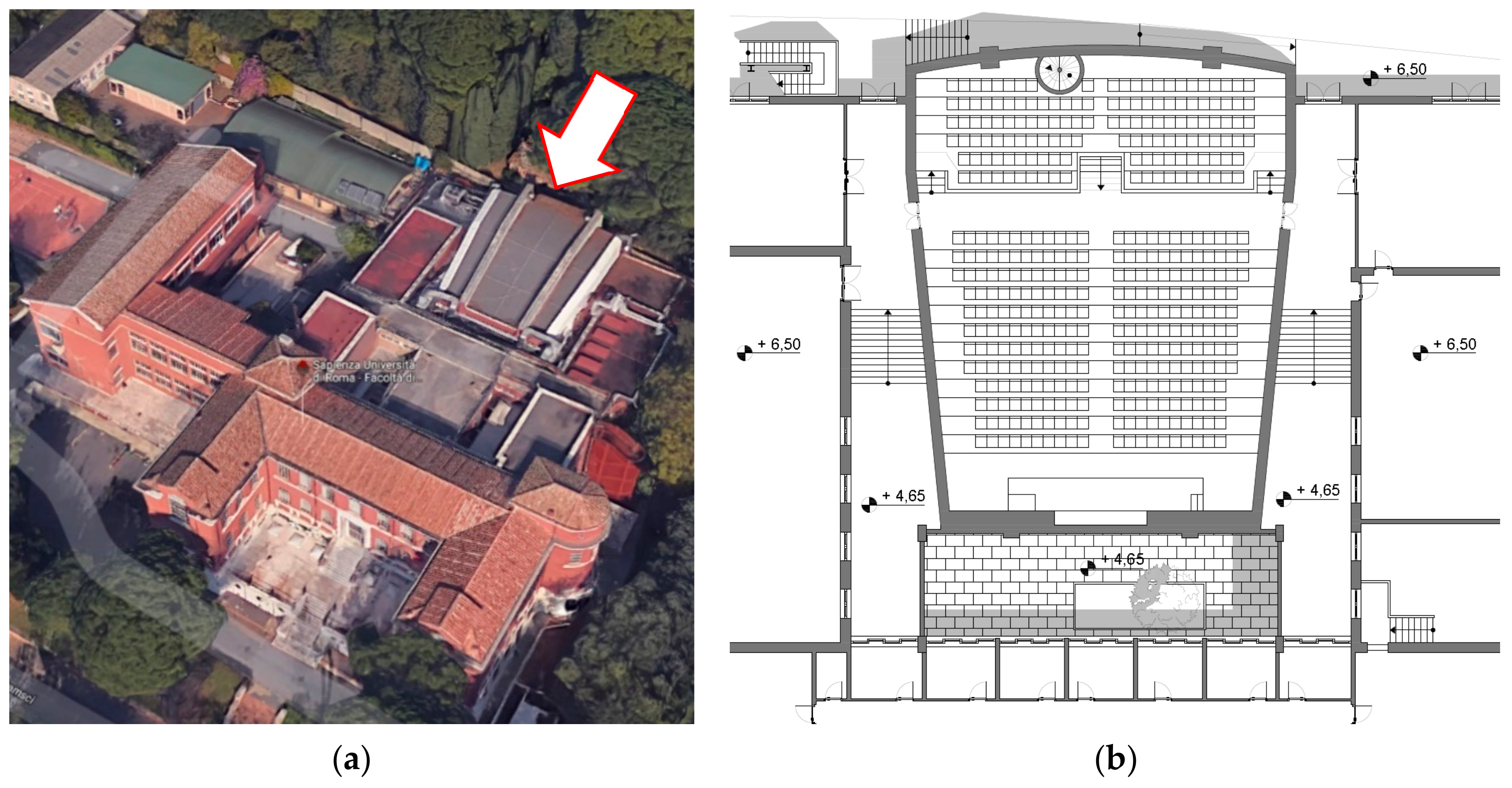
2.2. Case Study Description
- two days with morning lessons (occupancy 9 ÷ 12 a.m., HVAC system operation 8 ÷ 12 a.m.);
- two days with afternoon lessons (occupancy 14 ÷ 17 p.m., HVAC system start-up 13 ÷ 17 p.m.); and,
- one conference day (occupancy 9 a.m. ÷ 17 p.m., HVAC system start-up 8 a.m.÷ 17 p.m.).
3. Results and Discussion
3.1. Dynamic Simulation for Energy Savings
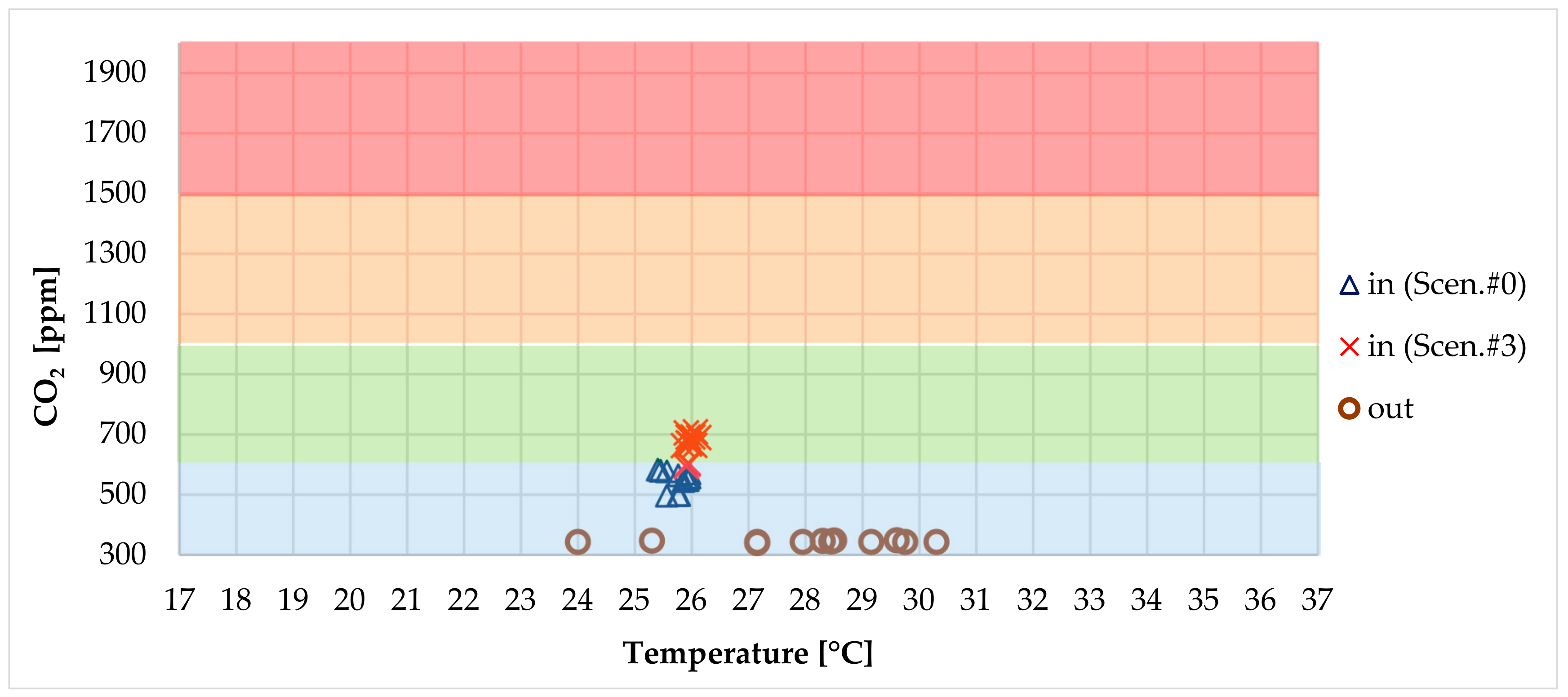
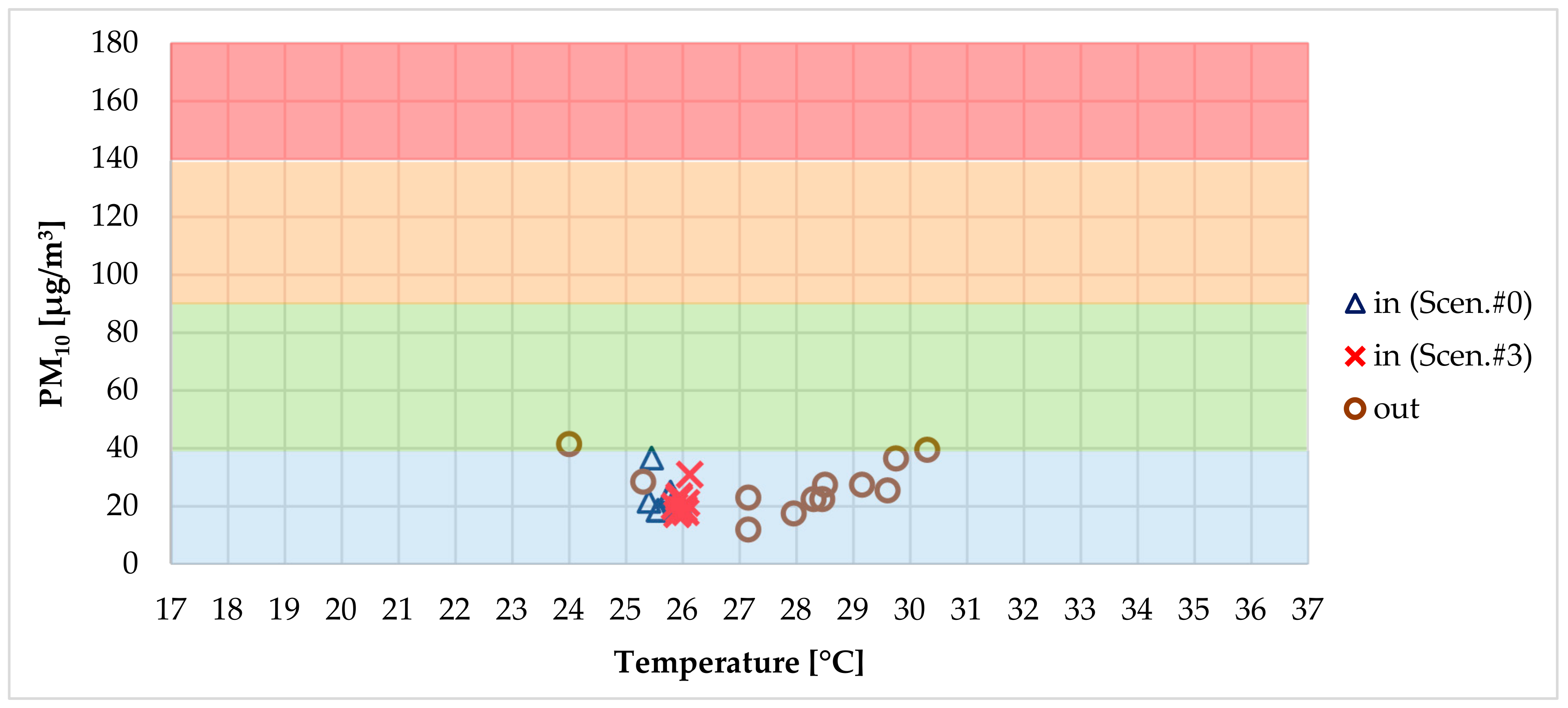
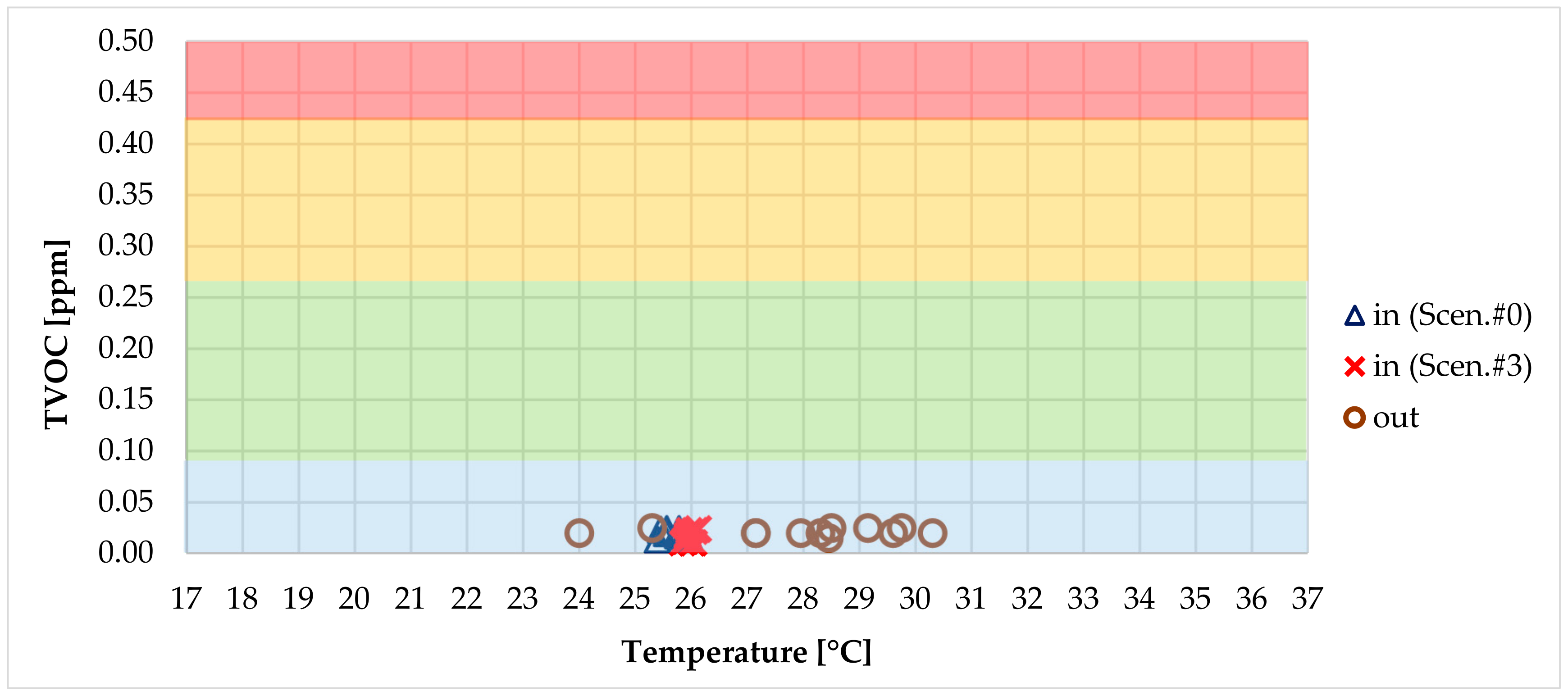
3.2. Measurement Campaign—Summer Operation
- Qsens and Qlat are the sensible and latent loads [W];
- G is the external airflow rate handled by the AHU [kg/s];
- cp is the specific heat at constant pressure, it can be considered constant and equal to 1005 J/(kgK);
- r is the heat of vaporization, it can be considered constant and equal to 2501 kJ/kg;
- TA and TS are the temperatures of the extracted air and the supply air, respectively [K]; and,
- xA and xS are the humidity ratio in the extracted air and in the supply air, respectively [g/kg].
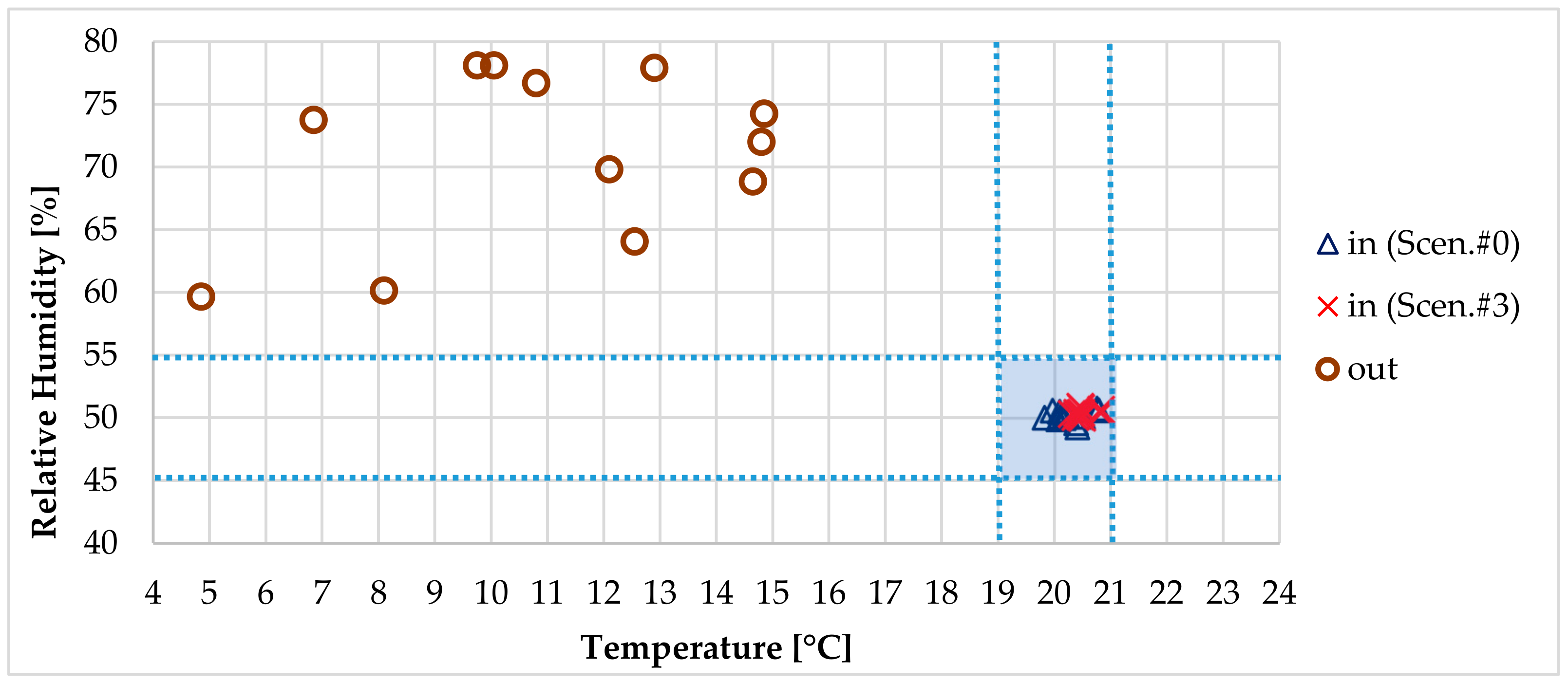
3.3. Measurement Campaign—Winter Operation
3.4. Discussion
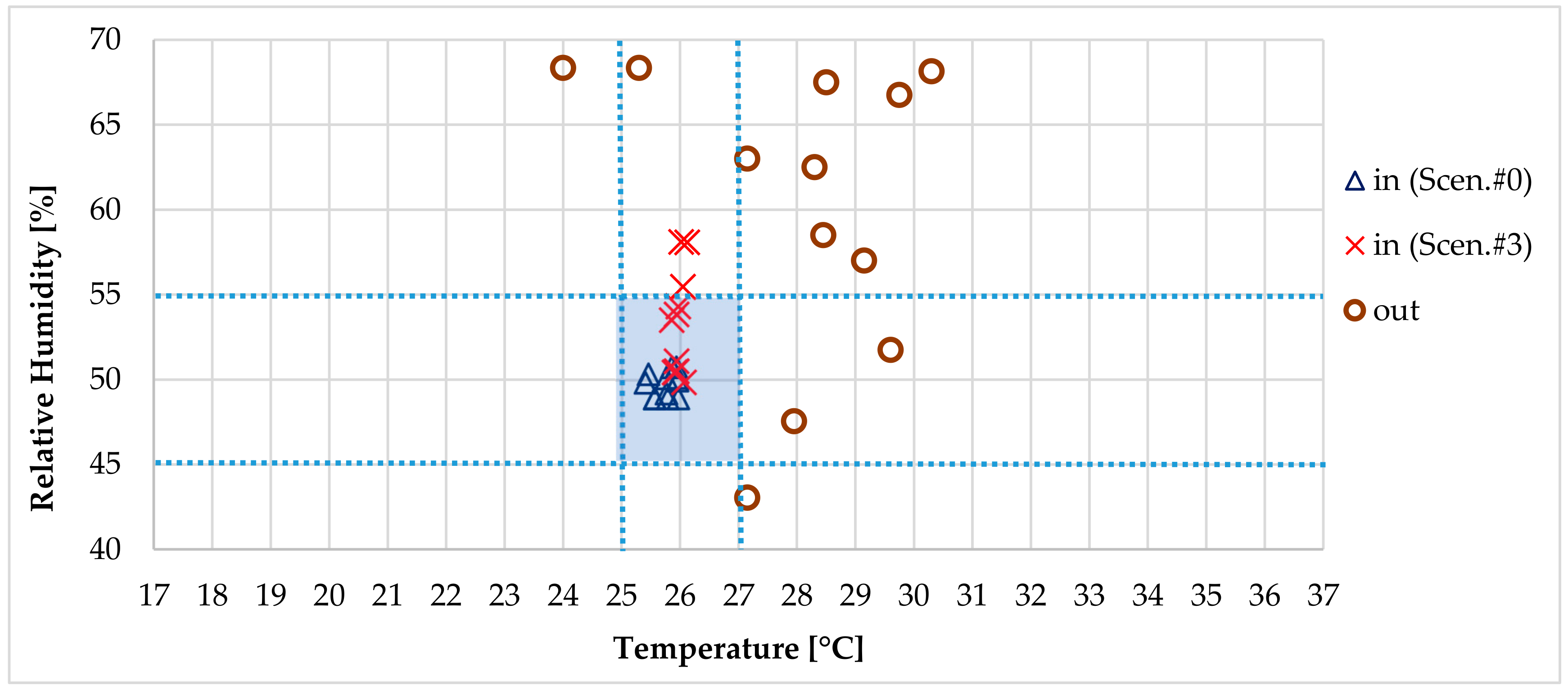
- the HVAC system is able to control the indoor temperature, even with half of the flow rate;
- in summer operation, the relative humidity was increased, due to the lesser ability of the system to dilute the water vapour linked to the decreased airflow rate, but was still acceptable (i.e., 53%);
- in winter operation, the HVAC system was able to maintain the relative humidity within the design range by humidifying the halved external airflow rate to a lesser extent;
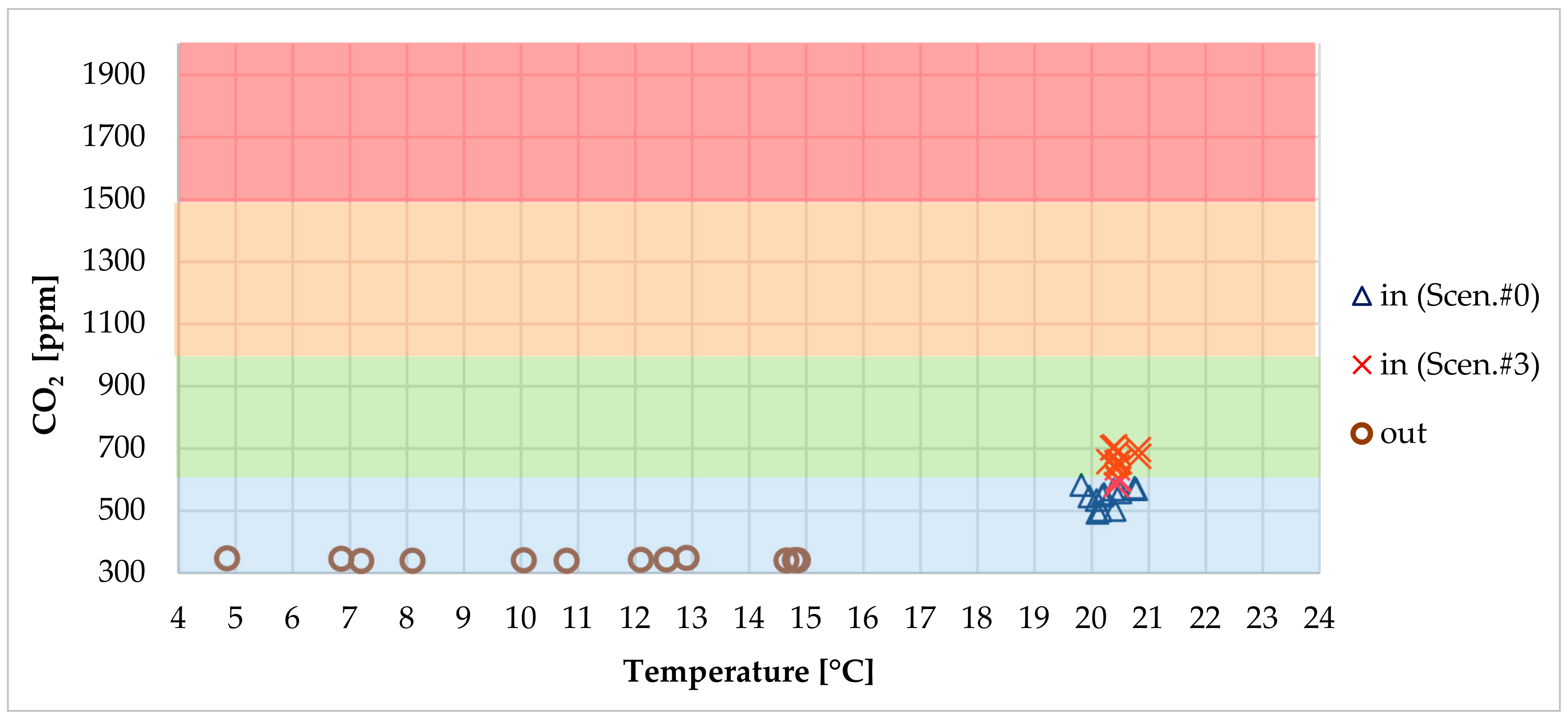
- CO2 concentration with 50% of the nominal airflow rate resulted to be higher but it is still within the moderate class, namely: it shifts from 539 ppm (good) to 663 ppm (moderate) in summer and from 539 ppm (good) to 647 ppm (moderate) in winter; and,
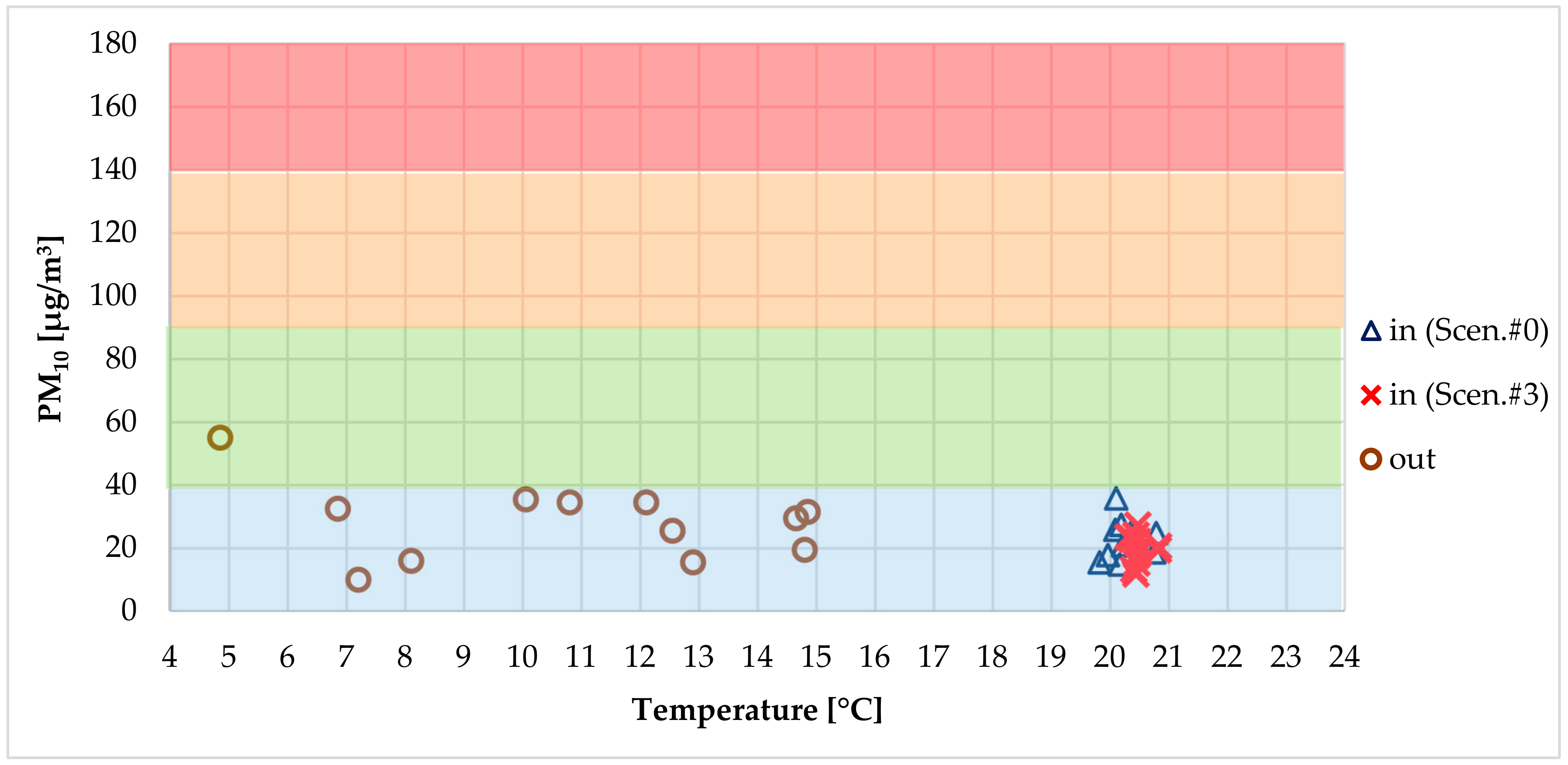
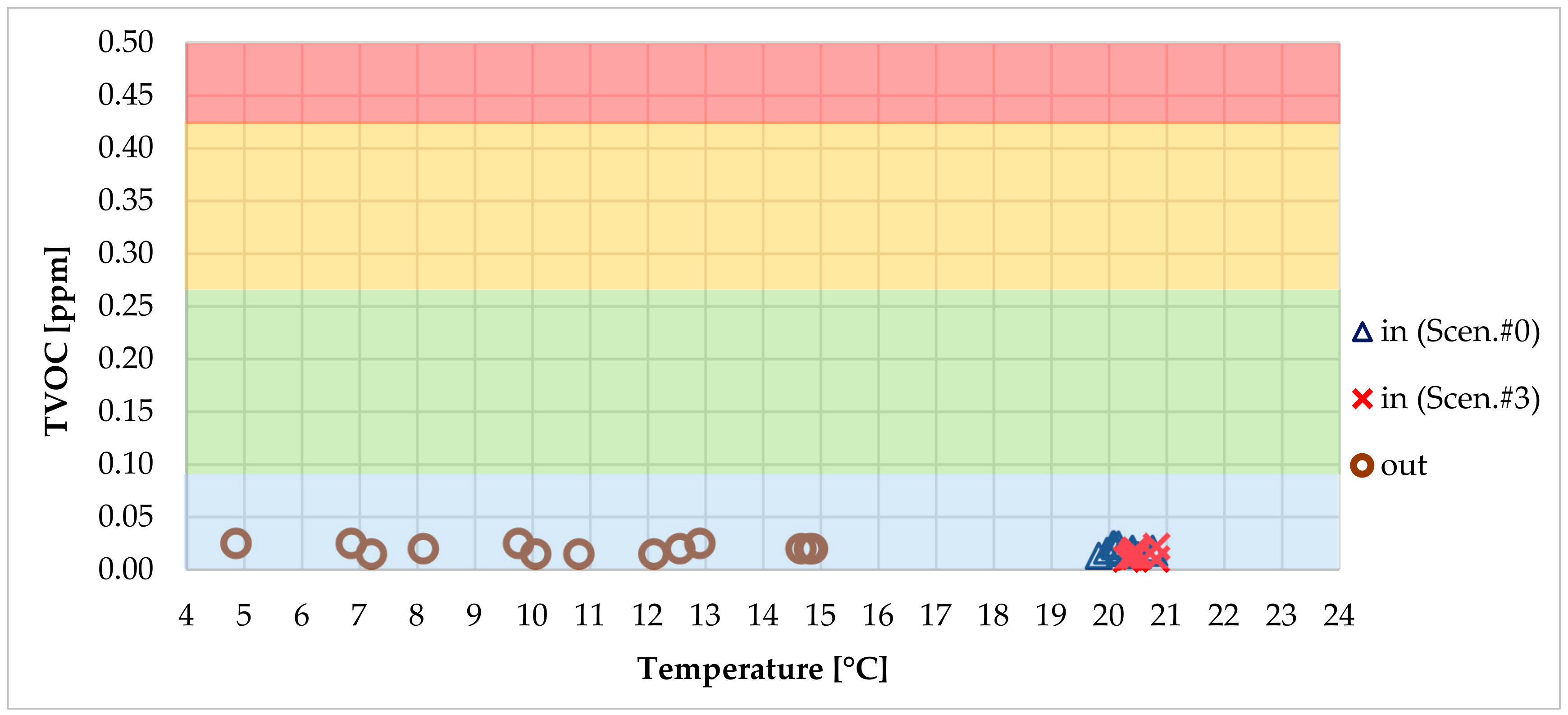
- concentration of other pollutants decreases proportionally with the airflow rate.
4. Conclusions
Author Contributions
Funding
Acknowledgments
Conflicts of Interest
References
- Soares, N.; Bastos, J.; Pereira, L.D.; Soares, A.; Amaral, A.R.; Asadi, E.; Rodrigues, E.; Lamas, F.B.; Monteiro, H.; Lopes, M.A.R.; et al. A review on current advances in the energy and environmental performance of buildings towards a more sustainable built environment. Renew. Sustain. Energy Rev. 2017, 77, 845–860. [Google Scholar] [CrossRef]
- Anderson, J.E.; Wulfhorst, G.; Lang, W. Energy analysis of the built environment—A review and outlook. Renew. Sustain. Energy Rev. 2015, 44, 149–158. [Google Scholar] [CrossRef]
- Frontczak, M.; Wargocki, P. Literature survey on how different factors influence human comfort in indoor environments. Build. Environ. 2011, 46, 922–937. [Google Scholar] [CrossRef]
- Al horr, Y.; Arif, M.; Katafygiotou, M.; Mazroei, A.; Kaushik, A.; Elsarrag, E. Impact of indoor environmental quality on occupant well-being and comfort: A review of the literature. Int. J. Sustain. Built Environ. 2016, 5, 1–11. [Google Scholar] [CrossRef]
- Wolkoff, P. Indoor air humidity, air quality, and health—An overview. Int. J. Hyg. Environ. Health 2018, 221, 376–390. [Google Scholar] [CrossRef]
- Kang, S.; Ou, D.; Mak, C.M. The impact of indoor environmental quality on work productivity in university open-plan research offices. Build. Environ. 2017, 124, 78–89. [Google Scholar] [CrossRef]
- Becker, R.; Goldberger, I.; Paciuk, M. Improving energy performance of school buildings while ensuring indoor air quality ventilation. Build. Environ. 2007, 42, 3261–3276. [Google Scholar] [CrossRef]
- De Santoli, L.; Garcia, D.A.; Groppi, D.; Bellia, L.; Palella, B.I.; Riccio, G.; Cuccurullo, G.; d’Ambrosio, F.R.; Stabile, L.; Dell’Isola, M.; et al. A General Approach for Retrofit of Existing Buildings Towards NZEB: The Windows Retrofit Effects on Indoor Air Quality and the Use of Low Temperature District Heating. In Proceedings of the 2018 IEEE International Conference on Environment and Electrical Engineering and 2018 IEEE Industrial and Commercial Power Systems Europe (EEEIC/I&CPS Europe), Palermo, Italy, 12–15 June 2018; IEEE: Piscataway, NJ, USA, 2018; pp. 1–6. [Google Scholar]
- Manfren, M.; Nastasi, B.; Piana, E.; Tronchin, L. On the link between energy performance of building and thermal comfort: An example. In Proceedings of the AIP Conference Proceedings (TMREES19), Beirut, Lebanon, 10–12 April 2019; AIP Publishing LLC: Melville, NY, USA, 2019; Volume 2123, p. 020066. [Google Scholar]
- Šujanová, P.; Rychtáriková, M.; Sotto Mayor, T.; Hyder, A. A Healthy, Energy-Efficient and Comfortable Indoor Environment, a Review. Energies 2019, 12, 1414. [Google Scholar] [CrossRef]
- Allab, Y.; Pellegrino, M.; Guo, X.; Nefzaoui, E.; Kindinis, A. Energy and comfort assessment in educational building: Case study in a French university campus. Energy Build. 2017, 143, 202–219. [Google Scholar] [CrossRef]
- Dias Pereira, L.; Neto, L.; Bernardo, H.; Gameiro da Silva, M. An integrated approach on energy consumption and indoor environmental quality performance in six Portuguese secondary schools. Energy Res. Soc. Sci. 2017, 32, 23–43. [Google Scholar] [CrossRef]
- Zuhaib, S.; Manton, R.; Griffin, C.; Hajdukiewicz, M.; Keane, M.M.; Goggins, J. An Indoor Environmental Quality (IEQ) assessment of a partially-retrofitted university building. Build. Environ. 2018, 139, 69–85. [Google Scholar] [CrossRef]
- Balocco, C.; Colaianni, A. Assessment of energy sustainable operations on a historical building. The Dante Alighieri high school in Florence. Sustainability 2018, 10, 2054. [Google Scholar] [CrossRef]
- De Santoli, L.; Mancini, F.; Rossetti, S.; Nastasi, B. Energy and system renovation plan for Galleria Borghese, Rome. Energy Build. 2016, 129, 549–562. [Google Scholar] [CrossRef]
- Legislative Decree no. 102/2014. Implementation of Directive 2012/27/EU. 2010, pp. 1–39. Available online: https://www.gazzettaufficiale.it/atto/vediMenuHTML;jsessionid=A+nWnzbPN4bZ5rVKTNAPXQ__.ntc-as2-guri2b?atto.dataPubblicazioneGazzetta=2014-07-18&atto.codiceRedazionale=14G00113&tipoSerie=serie_generale&tipoVigenza=originario (accessed on 1 December 2019).
- Mikučionienė, R.; Martinaitis, V.; Keras, E. Evaluation of energy efficiency measures sustainability by decision tree method. Energy Build. 2014, 76, 64–71. [Google Scholar] [CrossRef]
- Chung, M.H.; Rhee, E.K. Potential opportunities for energy conservation in existing buildings on university campus: A field survey in Korea. Energy Build. 2014, 78, 176–182. [Google Scholar] [CrossRef]
- Han, Y.; Zhou, X.; Luo, R. Analysis on Campus Energy Consumption and Energy Saving Measures in Cold Region of China. Procedia Eng. 2015, 121, 801–808. [Google Scholar] [CrossRef]
- Amber, K.P.; Aslam, M.W.; Mahmood, A.; Kousar, A.; Younis, M.Y.; Akbar, B.; Chaudhary, G.Q.; Hussain, S.K. Energy Consumption Forecasting for University Sector Buildings. Energies 2017, 10, 1579. [Google Scholar] [CrossRef]
- Congedo, P.; D’Agostino, D.; Baglivo, C.; Tornese, G.; Zacà, I. Efficient Solutions and Cost-Optimal Analysis for Existing School Buildings. Energies 2016, 9, 851. [Google Scholar] [CrossRef]
- Daisey, J.M.; Angell, W.J.; Apte, M.G. Indoor air quality, ventilation and health symptoms in schools: An analysis of existing information. Indoor Air 2003, 13, 53–64. [Google Scholar] [CrossRef]
- Zhong, L.; Yuan, J.; Fleck, B. Indoor Environmental Quality Evaluation of Lecture Classrooms in an Institutional Building in a Cold Climate. Sustainability 2019, 11, 6591. [Google Scholar] [CrossRef]
- Mihai, T.; Iordache, V. Determining the Indoor Environment Quality for an Educational Building. Energy Procedia 2016, 85, 566–574. [Google Scholar] [CrossRef]
- Almeida, R.M.S.F.; de Freitas, V.P. Indoor environmental quality of classrooms in Southern European climate. Energy Build. 2014, 81, 127–140. [Google Scholar] [CrossRef]
- Merema, B.; Delwati, M.; Sourbron, M.; Breesch, H. Demand controlled ventilation (DCV) in school and office buildings: Lessons learnt from case studies. Energy Build. 2018, 172, 349–360. [Google Scholar] [CrossRef]
- Aste, N.; Manfren, M.; Marenzi, G. Building Automation and Control Systems and performance optimization: A framework for analysis. Renew. Sustain. Energy Rev. 2017, 75, 313–330. [Google Scholar] [CrossRef]
- Mancini, F.; Lo Basso, G.; de Santoli, L. Energy Use in Residential Buildings: Impact of Building Automation Control Systems on Energy Performance and Flexibility. Energies 2019, 12, 2896. [Google Scholar] [CrossRef]
- Chenari, B.; Dias Carrilho, J.; Gameiro da Silva, M. Towards sustainable, energy-efficient and healthy ventilation strategies in buildings: A review. Renew. Sustain. Energy Rev. 2016, 59, 1426–1447. [Google Scholar] [CrossRef]
- Ben-David, T.; Waring, M.S. Impact of natural versus mechanical ventilation on simulated indoor air quality and energy consumption in offices in fourteen U.S. cities. Build. Environ. 2016, 104, 320–336. [Google Scholar] [CrossRef]
- Mui, K.W.; Wong, L.T.; Hui, P.S. Indoor Environmental Quality Benchmarks for Air-conditioned Offices in the Subtropics. Indoor Built Environ. 2009, 18, 123–129. [Google Scholar] [CrossRef]
- Wong, L.; Mui, K.; Tsang, T. Evaluation of Indoor Air Quality Screening Strategies: A Step-Wise Approach for IAQ Screening. Int. J. Environ. Res. Public Health 2016, 13, 1240. [Google Scholar] [CrossRef]
- Gabriel Rojas Rainer Pfluger, W.F. Ventilation concepts for energy efficient housing in Central European climate—A simulation study comparing indoor air quality, mould risk and ventilation losses. In Proceedings of the Indoor Air 2016, Ghent, Belgium, 3–8 July 2016. [Google Scholar]
- Karami, M.; McMorrow, G.V.; Wang, L. Continuous monitoring of indoor environmental quality using an Arduino-based data acquisition system. J. Build. Eng. 2018, 19, 412–419. [Google Scholar] [CrossRef]
- Vilčeková, S.; Apostoloski, I.; Mečiarová, Ľ.; Burdová, E.; Kiseľák, J. Investigation of Indoor Air Quality in Houses of Macedonia. Int. J. Environ. Res. Public Health 2017, 14, 37. [Google Scholar] [CrossRef] [PubMed]
- Bianco, V.; De Rosa, M.; Scarpa, F.; Tagliafico, L.A. Analysis of energy demand in residential buildings for different climates by means of dynamic simulation. Int. J. Ambient Energy 2016, 37, 108–120. [Google Scholar] [CrossRef]
- Mancini, F.; Cecconi, M.; De Sanctis, F.; Beltotto, A. Energy Retrofit of a Historic Building Using Simplified Dynamic Energy Modeling. Energy Procedia 2016, 101, 1119–1126. [Google Scholar] [CrossRef]
- De Santoli, L.; Mancini, F.; Clemente, C.; Lucci, S. Energy and technological refurbishment of the School of Architecture Valle Giulia, Rome. Energy Procedia 2017, 133, 382–391. [Google Scholar] [CrossRef]
- Chiesa, G.; Cesari, S.; Garcia, M.; Issa, M.; Li, S. Multisensor IoT Platform for Optimising IAQ Levels in Buildings through a Smart Ventilation System. Sustainability 2019, 11, 5777. [Google Scholar] [CrossRef]
- Kang, J.; Hwang, K.-I. A Comprehensive Real-Time Indoor Air-Quality Level Indicator. Sustainability 2016, 8, 881. [Google Scholar] [CrossRef]
- Hnat, T.W.; Srinivasan, V.; Lu, J.; Sookoor, T.I.; Dawson, R.; Stankovic, J.; Whitehouse, K. The hitchhiker’s guide to successful residential sensing deployments. In Proceedings of the SenSys 2011—9th ACM Conference on Embedded Networked Sensor Systems, Seattle, WA, USA, 1–4 November 2011; pp. 232–245. [Google Scholar]
- Pereira, P.F.; Ramos, N.M.M. The influence of sensor placement in the study of occupant behavior in a residential building. In Proceedings of the 2018 International Conference on Smart Energy Systems and Technologies (SEST), Sevilla, Spain, 10–12 September 2018; Institute of Electrical and Electronics Engineers Inc.: Piscataway, NJ, USA, 2018. [Google Scholar]
- UNI Ente Italiano di Normazione Italian technical standard UNI/TS 11300-1:2014—Energy Performance of Buildings—Evaluation of Energy Need for Space Heating and Cooling. Available online: http://store.uni.com/catalogo/index.php/uni-ts-11300-1-2014.html (accessed on 18 September 2019).
- Han, K.; Zhang, J.S.; Guo, B. A novel approach of integrating ventilation and air cleaning for sustainable and healthy office environments. Energy Build. 2014, 76, 32–42. [Google Scholar] [CrossRef]
- Noris, F.; Delp, W.W.; Vermeer, K.; Adamkiewicz, G.; Singer, B.C.; Fisk, W.J. Protocol for maximizing energy savings and indoor environmental quality improvements when retrofitting apartments. Energy Build. 2013, 61, 378–386. [Google Scholar] [CrossRef]
- Turner, W.J.N.; Logue, J.M.; Wray, C.P. A combined energy and IAQ assessment of the potential value of commissioning residential mechanical ventilation systems. Build. Environ. 2013, 60, 194–201. [Google Scholar] [CrossRef]
- Leivo, V.; Turunen, M.; Aaltonen, A.; Kiviste, M.; Du, L.; Haverinen-Shaughnessy, U. Impacts of Energy Retrofits on Ventilation Rates, CO2-levels and Occupants’ Satisfaction with Indoor Air Quality. Energy Procedia 2016, 96, 260–265. [Google Scholar] [CrossRef]


| Classes | CO2 [ppm] | TVOC [ppm] | PM10 [μg/m3] |
|---|---|---|---|
| Hazardous | 1501 ÷ 5000 | 0.431 ÷ 3000 | 141 ÷ 750 |
| Unhealthy | 1001 ÷ 1500 | 0.262 ÷ 0.430 | 91 ÷ 140 |
| Moderate | 601 ÷ 1000 | 0.088 ÷ 0.261 | 31 ÷ 90 |
| Good | 340 ÷ 600 | 0.000 ÷ 0.087 | 0 ÷ 30 |
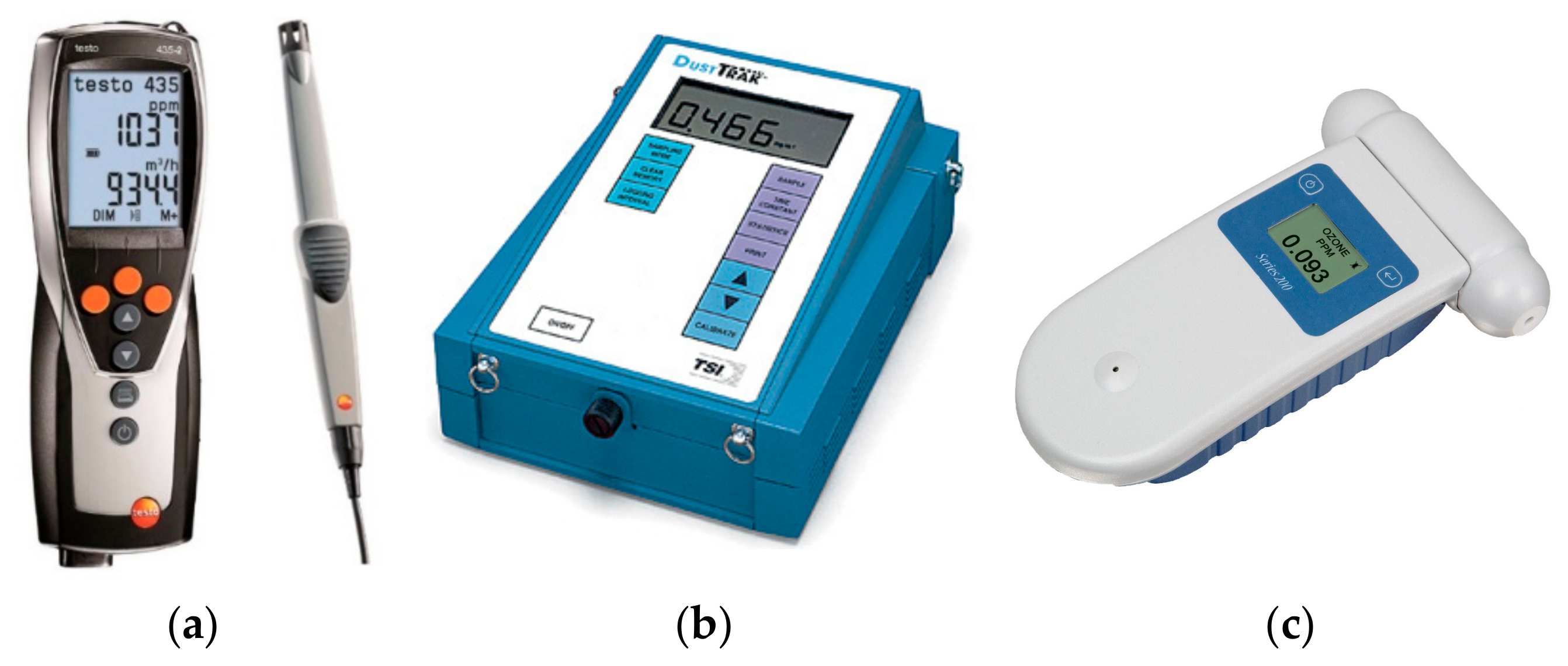
| Equipment | Parameter | Range | Resolution | Accuracy |
|---|---|---|---|---|
| Testo 435-2 | T | 0 to +50 °C | 0.1 °C | ±0.2 °C |
| Multifunction | RH | 0 to +100 %RH | 0.1 %RH | ±2%RH (98%RH) |
| IAQ meter | CO2 | 0 to +10,000 ppm | 1 ppm | ±(75 ppm ±3 % reading) |
| TSi DustTrak | PM10 | 0.001 to 100 mg/m3 | 0.001 mg/m3 | ±0.1% reading |
| Aerosol Monitor | or ±0.001 mg/m3 | |||
| Gas Detector Aeroqual AQ-200 | TVOC | 0 to 20 ppm | 0.01 ppm | ±10 % |
| Scenario | Relative Airflow Rate | Analysed Parameters | |
|---|---|---|---|
| Dynamic Simulation | Measurement Campaign | ||
| Scen. #0 | 100% | Energy consumptions; Thermal loads; T, RH | T; RH; CO2, PM10, TVOC concentrations |
| Scen. #1 | 85% | Energy consumptions; Thermal loads; T, RH | - |
| Scen. #2 | 70% | Energy consumptions; Thermal loads; T, RH | - |
| Scen. #3 | 50% | Energy consumptions; Thermal loads; T, RH | T; RH; CO2, PM10, TVOC concentrations |
| Pel [kW] | T indoor [°C] | RH [%] | |||||||
|---|---|---|---|---|---|---|---|---|---|
| Simulated | Measured | Error % | Simulated | Measured | Error % | Simulated | Measured | Error % | |
| 28-05 | 18.4 | 24.6 | 25.3 | 24.2 | 25.5 | 5.2 | 47.8 | 50.3 | 4.9 |
| 08-06 | 33.8 | 41.3 | 18.1 | 25.2 | 26.0 | 3.1 | 52.9 | 48.9 | −8.2 |
| 11-06 | 27.0 | 22.7 | −19.1 | 23.8 | 25.9 | 8.1 | 52.6 | 50.0 | −5.1 |
| 12-06 | 13.5 | 11.0 | −23.2 | 24.8 | 25.9 | 4.1 | 47.1 | 50.7 | 7.2 |
| 18-06 | 28.9 | 32.8 | 12.0 | 24.0 | 25.8 | 7.0 | 48.2 | 50.1 | 3.8 |
| 20-06 | 15.9 | 14.5 | −9.5 | 24.9 | 26.0 | 4.2 | 51.2 | 50.1 | −2.2 |
| 26-06 | 27.7 | 33.4 | 17.2 | 25.9 | 25.4 | −2.1 | 46.3 | 49.8 | 7.1 |
| 28-06 | 15.0 | 18.8 | 20.2 | 22.5 | 25.6 | 12.2 | 50.9 | 48.9 | −4.1 |
| 04-07 | 27.1 | 23.5 | −15.2 | 27.9 | 25.8 | −8.1 | 47.6 | 49.2 | 3.2 |
| 05-07 | 15.5 | 20.1 | 23.0 | 24.1 | 25.6 | 5.9 | 51.9 | 48.9 | −6.2 |
| 12-07 | 37.2 | 33.3 | −11.5 | 26.1 | 25.8 | −1.2 | 50.0 | 48.9 | −2.2 |
| 10-09 | 20.4 | 24.4 | 16.5 | 23.5 | 25.9 | 9.2 | 48.1 | 50.7 | 5.2 |
| Pel [kW] | T indoor [°C] | RH [%] | |||||||
|---|---|---|---|---|---|---|---|---|---|
| Simulated | Measured | Error % | Simulated | Measured | Error % | Simulated | Measured | Error % | |
| 07-11 | 12.5 | 15.7 | 20.2 | 20.0 | 20.8 | 3.8 | 48.2 | 50.8 | 5.2 |
| 09-11 | 12.6 | 15.5 | 18.8 | 21.7 | 20.8 | −4.1 | 47.0 | 50.6 | 7.2 |
| 14-11 | 17.6 | 15.1 | −16.5 | 21.9 | 20.2 | −8.2 | 53.5 | 50.4 | −6.1 |
| 16-11 | 16.1 | 18.5 | 13.0 | 21.0 | 20.2 | −4.1 | 47.7 | 50.2 | 4.9 |
| 21-11 | 15.5 | 12.3 | −25.1 | 21.2 | 20.0 | −6.1 | 54.7 | 50.6 | −8.1 |
| 23-11 | 15.6 | 19.8 | 21.2 | 22.0 | 20.5 | −7.2 | 48.2 | 50.1 | 3.8 |
| 28-11 | 20.0 | 17.2 | −16.1 | 20.8 | 19.8 | −5.2 | 51.7 | 50.1 | −3.1 |
| 05-12 | 25.8 | 21.9 | −18.2 | 21.0 | 20.4 | −3.1 | 47.0 | 49.6 | 5.2 |
| 07-12 | 24.3 | 30.3 | 19.9 | 20.0 | 20.4 | 2.1 | 46.9 | 49.3 | 4.9 |
| 12-12 | 23.6 | 20.0 | −18.2 | 21.3 | 20.1 | −6.2 | 54.2 | 50.1 | −8.1 |
| 14-12 | 14.4 | 18.2 | 21.0 | 21.3 | 20.2 | −5.2 | 46.4 | 50.0 | 7.1 |
| 19-12 | 23.9 | 28.8 | 17.3 | 20.7 | 20.1 | −3.1 | 51.8 | 50.5 | −2.6 |
| 21-12 | 16.9 | 14.2 | −19.0 | 20.9 | 20.1 | −4.1 | 47.5 | 49.9 | 4.9 |
| Qheat,average [kW] | Qheat,max [kW] | Eheat,TOT [kWh/y] | Pel,average [kW] | Pel,max [kW] | Eel,TOT [kWh/y] | ΔEel,TOT [%] | |
|---|---|---|---|---|---|---|---|
| Scen. #0 | 64.46 | 131.49 | 36,741 | 16.87 | 43.25 | 9618 | |
| Scen. #1 | 55.19 | 112.51 | 29,417 | 14.53 | 37.00 | 7745 | −19.5% |
| Scen. #2 | 45.44 | 93.39 | 23,176 | 11.94 | 30.78 | 6088 | −36.7% |
| Scen. #3 | 33.22 | 71.92 | 15,315 | 8.64 | 24.77 | 3984 | −58.6% |
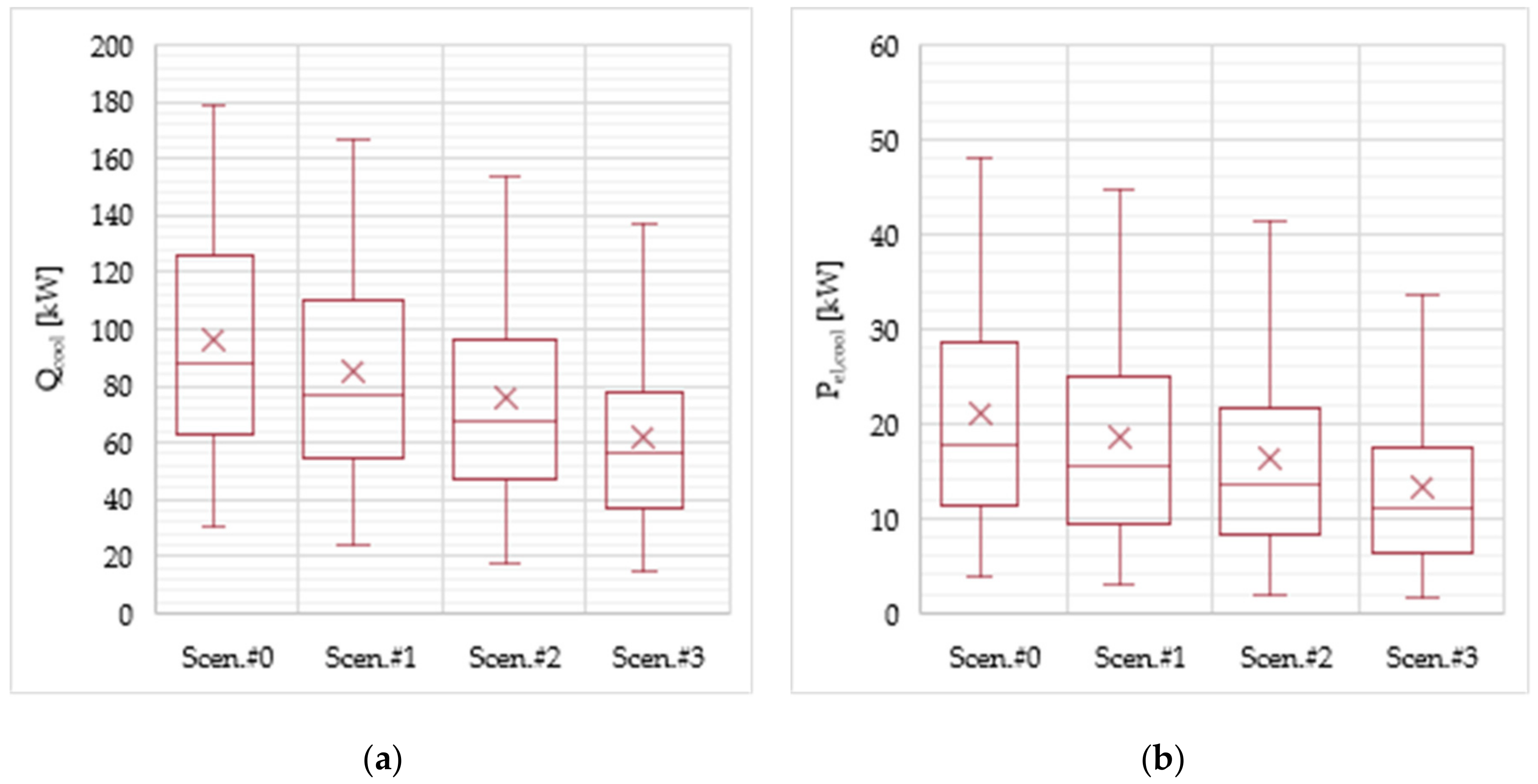
| Qcool,average [kW] | Qcool,max [kW] | Ecool,TOT [kWh/y] | Pel,average [kW] | Pel,max [kW] | Eel,TOT [kWh/y] | ΔEel,TOT | |
|---|---|---|---|---|---|---|---|
| Scen. #0 | 96.92 | 178.84 | 34,817 | 20.95 | 48.11 | 7604 | |
| Scen. #1 | 85.38 | 166.34 | 32,186 | 18.57 | 44.71 | 7000 | −7.9% |
| Scen. #2 | 75.47 | 153.85 | 29,282 | 16.36 | 41.31 | 6349 | −16.5% |
| Scen. #3 | 62.18 | 137.19 | 25,306 | 13.39 | 36.77 | 5451 | −28.3% |
| Date | Occup. | T; RH [°C; %] | CO2 [ppm] | PM10 [μg/m3] | TVOC [ppm] | ||||||||
|---|---|---|---|---|---|---|---|---|---|---|---|---|---|
| Out | In | In | Out | In | In | Out | In | In | Out | In | In | ||
| Sc. #0 | Sc. #3 | Sc. #0 | Sc. #3 | Sc. #0 | Sc. #3 | Sc. #0 | Sc. #3 | ||||||
| 28/05/2018 | 250 | 24; 68.4 | 25.5; 50.3 | 26.1; 58.1 | 344 | 580 | 690 | 41.5 | 36.7 | 31.0 | 0.020 | 0.023 | 0.024 |
| 08/06/2018 | 270 | 27.2; 63 | 26; 48.9 | 26; 58.1 | 340 | 557 | 692 | 23.0 | 20.0 | 19.2 | 0.020 | 0.016 | 0.010 |
| 11/06/2018 | 250 | 28.5; 58.5 | 25.9; 50 | 26; 54.3 | 345 | 556 | 669 | 22.5 | 20.1 | 18.8 | 0.015 | 0.016 | 0.022 |
| 12/06/2018 | 250 | 28.3; 62.5 | 25.9; 50.7 | 26.1; 55.5 | 347 | 548 | 664 | 22.5 | 19.9 | 18.0 | 0.020 | 0.015 | 0.010 |
| 18/06/2018 | 300 | 28.5; 67.5 | 25.8; 50.1 | 25.9; 50.5 | 348 | 564 | 691 | 27.5 | 23.6 | 23.5 | 0.025 | 0.018 | 0.018 |
| 20/06/2018 | 250 | 29.6; 51.8 | 26; 50.1 | 25.9; 53.9 | 349 | 571 | 672 | 25.5 | 20.6 | 18.7 | 0.020 | 0.014 | 0.017 |
| 26/06/2018 | 300 | 28; 47.6 | 25.4; 49.8 | 26.1; 49.9 | 344 | 583 | 709 | 17.5 | 21.7 | 21.2 | 0.020 | 0.013 | 0.022 |
| 28/06/2018 | 270 | 27.2; 43.1 | 25.6; 48.9 | 25.9; 50.5 | 343 | 578 | 705 | 12.0 | 18.6 | 17.3 | 0.020 | 0.024 | 0.013 |
| 04/07/2018 | 250 | 30.3; 68.2 | 25.8; 49.2 | 25.9; 51.1 | 343 | 499 | 606 | 39.5 | 24.0 | 22.7 | 0.020 | 0.018 | 0.017 |
| 05/07/2018 | 230 | 29.8; 66.8 | 25.6; 48.9 | 25.9; 50.5 | 343 | 497 | 594 | 36.5 | 18.6 | 17.3 | 0.025 | 0.020 | 0.012 |
| 12/07/2018 | 200 | 29.2; 57 | 25.8; 48.9 | 25.9; 50.5 | 343 | 499 | 602 | 27.5 | 25.0 | 22.8 | 0.025 | 0.024 | 0.015 |
| 10/09/2018 | 250 | 25.3; 68.4 | 25.9; 50.7 | 25.9; 53.5 | 348 | 545 | 663 | 28.5 | 22.5 | 20.0 | 0.025 | 0.017 | 0.010 |
| Data | Occup. | T; RH [°C; %] | CO2 [ppm] | PM10 [μg/m3] | TVOC [ppm] | ||||||||
|---|---|---|---|---|---|---|---|---|---|---|---|---|---|
| Out | In | In | Out | In | In | Out | In | In | Out | In | In | ||
| Sc. #0 | Sc. #3 | Sc. #0 | Sc. #3 | Sc. #0 | Sc. #3 | Sc. #0 | Sc. #3 | ||||||
| 07/11/2018 | 250 | 14.8; 72 | 20.8; 50.8 | 20.8; 50.7 | 342 | 573 | 675 | 19.5 | 18.7 | 20.6 | 0.020 | 0.020 | 0.022 |
| 09/11/2018 | 280 | 14.7; 68.9 | 20.8; 50.6 | 20.8; 50.4 | 340 | 569 | 696 | 29.5 | 24.8 | 19.5 | 0.020 | 0.016 | 0.010 |
| 14/11/2018 | 240 | 12.1; 69.8 | 20.2; 50.4 | 20.4; 50.2 | 342 | 549 | 653 | 34.5 | 27.4 | 24.2 | 0.015 | 0.016 | 0.018 |
| 16/11/2018 | 300 | 12.6; 64.1 | 20.2; 50.2 | 20.5; 50.2 | 343 | 554 | 688 | 25.5 | 20.9 | 17.8 | 0.020 | 0.017 | 0.013 |
| 21/11/2018 | 200 | 12.9; 77.9 | 20; 50.6 | 20.5; 50.9 | 348 | 545 | 638 | 15.5 | 17.8 | 15.3 | 0.025 | 0.018 | 0.018 |
| 23/11/2018 | 220 | 14.9; 74.3 | 20.5; 50.1 | 20.5; 50.1 | 341 | 559 | 658 | 31.5 | 20.6 | 18.7 | 0.020 | 0.014 | 0.017 |
| 28/11/2018 | 280 | 8.1; 60.2 | 19.8; 50.1 | 20.4; 50.4 | 340 | 582 | 705 | 16.0 | 15.5 | 13.2 | 0.020 | 0.013 | 0.014 |
| 05/12/2018 | 300 | 10.8; 76.7 | 20.4; 49.6 | 20.4; 50.1 | 340 | 567 | 702 | 34.5 | 26.0 | 22.8 | 0.015 | 0.018 | 0.012 |
| 07/12/2018 | 250 | 10.1; 78.1 | 20.4; 49.3 | 20.5; 50.8 | 341 | 502 | 604 | 35.5 | 24.2 | 22.2 | 0.015 | 0.020 | 0.015 |
| 12/12/2018 | 270 | 4.9; 59.7 | 20.1; 50.1 | 20.5; 50.5 | 347 | 493 | 599 | 55.0 | 35.8 | 27.3 | 0.025 | 0.022 | 0.017 |
| 14/12/2018 | 180 | 7.2; 90 | 20.2; 50 | 20.4; 50.4 | 339 | 501 | 583 | 10.0 | 14.8 | 11.8 | 0.015 | 0.024 | 0.015 |
| 19/12/2018 | 270 | 6.9; 73.8 | 20.1; 50.5 | 20.3; 50.4 | 346 | 534 | 657 | 32.5 | 25.9 | 23.5 | 0.025 | 0.024 | 0.010 |
| 21/12/2018 | 160 | 9.8; 78.1 | 20.1; 49.9 | 20.4; 50.3 | 341 | 480 | 555 | 37.5 | 33.4 | 31.0 | 0.025 | 0.024 | 0.015 |
© 2020 by the authors. Licensee MDPI, Basel, Switzerland. This article is an open access article distributed under the terms and conditions of the Creative Commons Attribution (CC BY) license (http://creativecommons.org/licenses/by/4.0/).
Share and Cite
Mancini, F.; Nardecchia, F.; Groppi, D.; Ruperto, F.; Romeo, C. Indoor Environmental Quality Analysis for Optimizing Energy Consumptions Varying Air Ventilation Rates. Sustainability 2020, 12, 482. https://doi.org/10.3390/su12020482
Mancini F, Nardecchia F, Groppi D, Ruperto F, Romeo C. Indoor Environmental Quality Analysis for Optimizing Energy Consumptions Varying Air Ventilation Rates. Sustainability. 2020; 12(2):482. https://doi.org/10.3390/su12020482
Chicago/Turabian StyleMancini, Francesco, Fabio Nardecchia, Daniele Groppi, Francesco Ruperto, and Carlo Romeo. 2020. "Indoor Environmental Quality Analysis for Optimizing Energy Consumptions Varying Air Ventilation Rates" Sustainability 12, no. 2: 482. https://doi.org/10.3390/su12020482
APA StyleMancini, F., Nardecchia, F., Groppi, D., Ruperto, F., & Romeo, C. (2020). Indoor Environmental Quality Analysis for Optimizing Energy Consumptions Varying Air Ventilation Rates. Sustainability, 12(2), 482. https://doi.org/10.3390/su12020482