Impact of COVID-19 on Urban Mobility during Post-Epidemic Period in Megacities: From the Perspectives of Taxi Travel and Social Vitality

Abstract

The prevention and control of COVID-19 in megacities is under large pressure because of tens of millions and high-density populations. The majority of epidemic prevention and control policies implemented focused on travel restrictions, which severely affected urban mobility during the epidemic. Considering the impacts of epidemic and associated control policies, this study analyzes the relationship between COVID-19, travel of residents, Point of Interest (POI), and social activities from the perspective of taxi travel. First, changes in the characteristics of taxi trips at different periods were analyzed. Next, the relationship between POIs and taxi travels was established by the Geographic Information System (GIS) method, and the spatial lag model (SLM) was introduced to explore the changes in taxi travel driving force. Then, a social activities recovery level evaluation model was proposed based on the taxi travel datasets to evaluate the recovery of social activities. The results demonstrated that the number of taxi trips dropped sharply, and the travel speed, travel time, and spatial distribution of taxi trips had been significantly influenced during the epidemic period. The spatial correlation between taxi trips was gradually weakened after the outbreak of the epidemic, and the consumption travel demand of people significantly decreased while the travel demand for community life increased dramatically. The evaluation score of social activity is increased from 8.12 to 74.43 during the post-epidemic period, which may take 3–6 months to be fully recovered as a normal period. Results and models proposed in this study may provide references for the optimization of epidemic control policies and recovery of public transport in megacities during the post-epidemic period.

1. Introduction

The abrupt COVID-19 epidemic has disrupted the normal economic and social development in China and throughout the world, especially for megacities because of their large populations [1,2]. Strict epidemic control measures have been adopted in many cities such as lockdown and work suspension because of the necessity of epidemic prevention and control, which have played an important role in controlling the rapid and large-scale spread of COVID-19 [3,4,5,6]. Undoubtedly, those epidemic control policies reduced the number of social and economic activities and had significant impacts on urban transport systems such as the sudden decrease of trips and the change of travel mode. Recently, the epidemic situation has been gradually alleviated and the economic and social recovery plan has been put on the agenda by the government during the post epidemic period. Under this circumstance, urban transport system plays a crucial role in the process of social recovery and economic recovery as the basic guarantee of the city. Therefore, more attentions should be paid on the impacts of the epidemic on urban transport system as well as the travel behavior.

Human beings have taken the most extensive and strict control measures to face the unprecedented epidemic. Infectious diseases are a major problem in public health prevention because of its high contagiousness. Therefore, it is essential to control or block the spread of virus from person-to-person and treat the infected person with entire efforts [7,8,9]. Based on the experiences from another epidemic in 2002 called SARS (Severe Acute Respiratory Syndrome), many similar measures were applied at the beginning of the prevention and control of COVID-19, such as active case screening, contact tracing, isolation of infected people and all associated contacts, social distancing, and community containment [10]. In fact, countries or regions that have been seriously affected by SARS are more experienced in coping with COVID-19. Control measures adopted by China have quickly alleviated the spread of the virus [11]. Some other studies have demonstrated the significance of the control measures applied during the first 50 days and suggested that Hubei Province and other megacities in China should extend their control periods [12,13]. Many traditional public health control measures such as isolation and quarantine, social distancing, and community containment could be applied for the prevention and control of large-scale spread of COVID-19 [14]. At the same time, it is also effective to strengthen hospital surveillance and infection control [15], reduce the contact rate of susceptible and infected residents, and isolate the infected people [16]. An extension of the traffic control bundling has been proved to be able to interrupt the community-hospital-community transmission cycle and thus reduce the impact of COVID-19 [17]. Research on epidemic specific containment measures and death rates in European countries showed that the speed of response along with the decision to suspend international flights might determine the impact of epidemic outbreak on fatality [18].

The essence of epidemic control measures is to restrict the movement and gathering of people which can normally be conducted by travel restrain. Statistical data have indicated that the number of national railway, highway, waterway, and civil aviation passengers in China during the Spring Festival in 2020 is only 49.7% of that number in 2019 [19]. Meanwhile, the operation of urban public transport travels were significantly affected by the epidemic. For example, bus and urban rail transit have taken certain measures which includes the reduction of frequency, extension of departure interval, and adjustment of operation time based on the travel demand. Therefore, the total passenger traffic in central cities across China in February 2020 was 50.3% of the same period in 2019, which continuously decreased to 43.4% in March 2020 [20]. Public transport users have dropped by more than 90% in some European cities [4,21]. Interestingly, some studies have demonstrated that the interventions to control the COVID-19 outbreak led to an improvement of air quality which could bring health benefits for non-COVID-19 deaths and potentially outnumber the confirmed deaths caused by COVID-19 in China [22].

Several concerns about the impacts of the epidemic on transport system and travel behavior are emerged after the outbreak of COVID-19. For example, many scholars are interested in the differences in the travel behavior of residents compared to the normal period and what factors may affect the travel behavior of residents as well as the level of economic and social recovery in the post epidemic period. Huang et al. quantified the impact of COVID-19 on transportation-related behaviors of the public based on the navigation record, indicating that the COVID-19 epidemic did cause a great impact on transportation-related behaviors of the public in Mainland China [23]. Wilbur et al. founded that there was a significant difference in ridership decline between the highest-income areas and lowest-income areas (77% vs. 58%) in Nashville, and they believed that the epidemic has a greater impact on low-income groups [24]. Arellana et al. used official and secondary data from the top seven most populated cities in Colombia to analyze the impacts on air transport, freight transport, and urban transport. The results showed that national policies and local decisions have reduced the demand for the transport system [25].

The travel mode choice behavior was also influenced by the epidemic. During the epidemic period, people try to avoid crowded places because they are required to keep a social distance. However, since it is difficult to satisfy the requirement of a social distance of more than 2 meters on most public transport vehicles, many people treat public transport as an unsafe transport mode during the epidemic period [24]. It is obvious to all that the trips of public transport decreased dramatically during the epidemic period, and many researchers believe that the trips of public transport will maintain a low level for a long time, which will be replaced by the increase of other transport modes such as private vehicles, non-motorized vehicles, and walking [26]. Public transport must change the impression of insecurity for attracting more passengers, and it is necessary for the government to strengthen the policy support for public transport in the post epidemic period because public transport has a great impact on many social issues, such as social equity and sustainable development [27].

The assessment of the impact of the epidemic on public transport and social economy is very important for the reconstruction work in the post epidemic period. The economic development has been slowed down and the transport industry has been seriously impacted due to the epidemic [28]. It is difficult to predict what the city will look like after the epidemic, but it is assured that the economic recovery will not be achieved overnight [29]. Meanwhile, it is necessary to assess the extent of socio-economic and transport impacts caused by the epidemic for the better guidance of the economic recovery. Tang et al. proposed a Bayesian Network Model based on a function-oriented resilience framework and ontological interdependence among 10 system qualities to probabilistically assess the general resilience of the road transport system in Beijing from 1997 to 2016 [30]. A resilient transport system will enhance its ability to resist risks and ensure that it can continue to play a role under the influence of emergencies. Resilient and sustainable infrastructure will continue to be critical to addressing evolving natural and man-made hazards in the 21st Century [31]. Wang et al. applied the complex network theory to establish a model of air sector network in China and examined a series of characteristic parameters with an empirical analysis on its vulnerability and resilience [32]. From the perspective of mobility, Huang et al. proposed two new economic indicators as the complementary measures to domestic investments and consumption activities by using data from Baidu Maps [33]. Gössling et al. analyzed the long-term impact of the epidemic on tourism and discusses the recovery assessment of tourism in the future [34]. Dang et al. evaluated the economic recovery of Vietnam in the post epidemic period. A web-based rapid assessment survey was implemented and analyzed in Vietnam to investigate household finance and future economic expectations in developing countries [35].

As an important supplement of public transport in most megacities, taxies can record the exact time and location of departure and arrival, and the boarding and alighting locations of taxi passengers are closer to the origin and destination of trips compared to other public transport modes [36]. The 24-h continuous operation of taxies can reflect the demand and dynamic change of urban traffic [37]. Therefore, it is more suitable to use data of taxi travel to conduct the travel temporal-spatial analysis based on the several reasons mentioned above. Point of interest (POI) is the precise positioning of urban function points, which has been proved to have a strong correlation with travel behaviors [38]. Taxi trajectory data combined with POI data is usually used to analyze the relationship between travel behavior and urban land use in many studies [39,40].

Most recent research which studied the interaction between COVID-19 and mobility mainly focused on the impact of the epidemic on the travel trips by analyzing the changes of number of trips between the normal period and the epidemic period. However, fewer studies were conducted on the changes in the temporal and spatial dimension of travel. Meanwhile, it is widely believed that the travel behavior of residents is strongly related to social activities and epidemic control policies during the epidemic period. In this case, we hope to explore the impacts of different control policies on travel behavior during the epidemic period in this study. Moreover, the main driving factors of travel and the changes occurred with the impact of urban land use are also investigated. The answers to these questions are of great importance to the improvement of epidemic prevention and control as well as the planning and construction of sustainable cities and sustainable transport in the future. Current transport related research during the epidemic period mainly focused on the changes of trips such as bus, rail transit, and aviation. However, there are still many restrictions on these modes of transport, such as the limitations on travel time and travel area. For example, most public transport vehicles usually stop operating at night and cannot reach anywhere in the city. Therefore, it is novel and creative to study the impact of COVID-19 on travel behavior and transport system from the perspective of taxi trips.

In addition, the epidemic has had a serious impact on the economy that the average income of people have dropped sharply and many people even lost their jobs [41,42,43]. Under this circumstance, economic recovery is treated as the primary task for the post epidemic period. Compared to the assessment based on investigation or statistics which is usually expensive and time-costing, it is important to formulate the economic policies by evaluating the social vitality in a relatively short time.

By considering several research gaps mentioned above, this paper analyzes the impact of COVID-19 on travel of people from the perspective of taxi travel and epidemic control policies. First, changes in the characteristics of taxi trips at each period of the epidemic were analyzed. Next, the relationship between POIs and taxi travels was established by the GIS method, and the spatial lag model (SLM) was introduced to explore the changes in taxi travel driving force. Finally, a social activities recovery level evaluation model was proposed based on the taxi travel datasets to evaluate the recovery level of social activities.

The implications and contributions of this study are summarized as follows:

This paper supplements the lack of research on the impact of COVID-19 on taxi travel and enriches the research on the impact of the epidemic on urban traffic. Due to the fact that the taxi has the advantages of 24-h operation and can operate in any area of the city, the scope of time and space for this research is expanded and travel characteristics of residents are captured in the whole day and the whole city to study the spatial and temporal changes of taxi trips. Moreover, operation information included in the taxi datasets are used to study the change of taxi operation and analyze the degree and trend of the impact of the epidemic on the income of drivers.

In this study, the trip information and travel behavior are related to POI by the GIS method. The spatial econometric model is introduced to evaluate the change of taxi travel driving force and the relationship between the spatial-temporal evolution of travel and urban functional structure during the epidemic period. A previous study mentioned that POIs have numerous attribute information which are related to the types of land use [44]. Therefore, POIs can accurately represent the distribution characteristics of urban function points and have a strong correlation with travel purpose [45]. Moreover, this study is able to study the relationship between the distribution of POI and origin and destination of taxi trips because the spatial information of taxi travel is also included in taxi datasets. Since the construction of the social activity recovery level evaluation model during the post epidemic period is only relied on the travel data of taxi, this study also proposed an alternative model which can evaluate the recovery level with relatively small data sample.

The rest of the paper is organized as follows. Section 2 introduces the research framework and describes the study area and the process of data cleaning. The model selection and variable selection for each part of the study is also included in this section. Section 3 presents the model results and discusses the main findings. Section 4 summarizes the theoretical implications and practical implications of this study. Limitations and suggestions for future study are also provided at the end of this section.

2. Materials and Methods

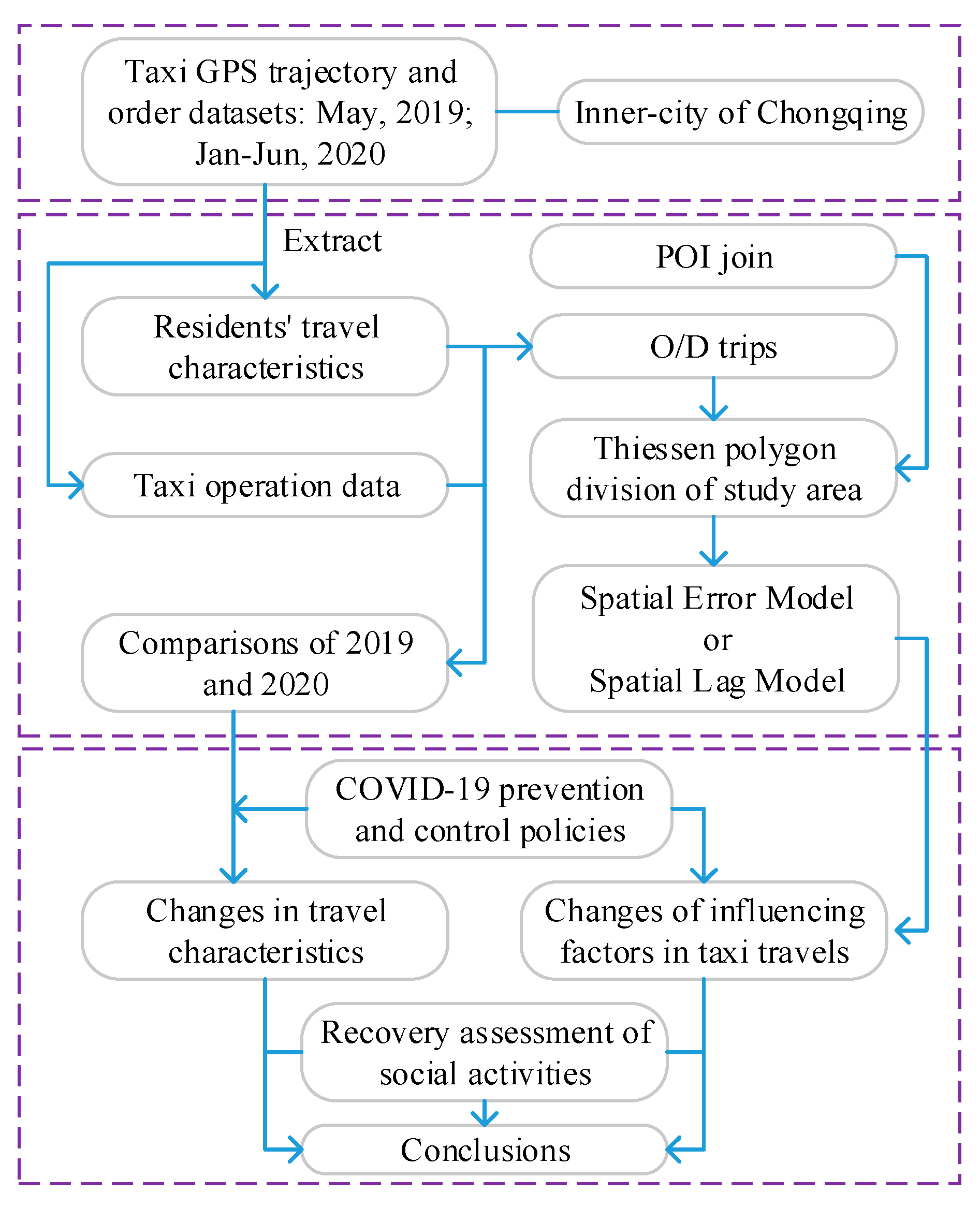
2.1. Research Framework

The research framework of this study is composed of three parts, as shown in Figure 1. First, the data source and study area are determined and the essential datasets for the study are figured out. Then, the characteristics of taxi travel between different periods are compared, and the spatial correlation between POI and taxi travels is established. Meanwhile, the POI driving force influence model of taxi travel and social activity recovery evaluation model are constructed respectively. Furthermore, the changes in taxi travel characteristics are analyzed and the model results are presented and discussed. Finally, the recommendations for a sustainable public transport system are provided.

2.2. Study Area and Data

2.2.1. Study Area

In order to analyze the impacts of COVID-19 on taxi usage behaviors in megacities, the empirical study is conducted by using the data from the central districts of Chongqing, one of the four centrally-administered municipalities in China with the city area of 5472.5 km² and a permanent population of 8.75 million by 2018 [46].

2.2.2. Data Description

•  Taxi trip datasets

The taxi trip dataset used in this study includes taxi trajectory datasets and taxi order datasets of 2862 taxies and 8738 drivers in Chongqing. All the data are obtained from the largest taxi company in Chongqing which operates more than half of the taxies in the city.

The original taxi order dataset records the operation information of taxies and drivers such as the vehicle ID, driver license number, order start time, order end time, order duration, and order fare. The taxi trajectory dataset includes the vehicle trajectory data recorded by their on-board terminals every 15 s such as vehicle ID, positioning time, longitude, latitude, instantaneous speed, direction angle, and taxi operating status. Taxi trip datasets of January to June 2020 are selected for the epidemic period and datasets of May 2019 are selected as the normal period for comparison.

•  Data cleaning and pre-processing treatment

Once we obtained the original datasets from the taxi company, the data cleaning and pre-processing treatment was conducted by eliminating invalid samples. The defective data with missing items or abnormal attributes such as extremely long continuous trips and long continuous trips with the low fare were removed from the taxi order datasets. For the taxi trajectory datasets, data with missing items, excessive speed between adjacent GPS points and data with incomplete origin or destination were also removed from the datasets [47].

After the data processing, the number of trips, trip start time, occupied hours and vacant hours of taxi operation, as well as the monthly income of drivers and taxies are obtained from the taxi order datasets. Meanwhile, information about travel distance, travel time, travel speed, origin, and destination of trips are collected from the trajectory datasets.

•  POI dataset

POI refers to the point of information or point of interest in geometric information system and map service. In this study, we collected all 15 types of POI data from Amap, one of the most popular map applications in China, and then reclassified the POI data into 7 categories including Business_Government, Consumption, Leisure, Medical_Services, Residential_Quarter, Services_Around, and Transportation. The original 17 categories and their associated new categories are shown in

Table 1. Point of Interest (POI) reclassification.

Index	Original Category	New Category	Index
1	Hotel	Consumption	1
2	Catering
3	Shopping
4	Enterprise	Business_Government	2
5	Business Building
6	Government
7	Entertainment	Leisure	3
8	Tourist Attractions
9	Medical Treatment and Public Health	Medical_Services	4
10	Residential Community	Residential_Quarter	5
11	Life Services	Services_Around	6
12	Auto Service
13	Finance
14	Roads	Transportation	7
15	Transport infrastructure

. The attributes of POI include location, name, longitude, latitude, address, phone number, and category.

The defective POI data such as missing attribute information, duplicate records, or beyond the research area was removed and finally 238,090 valid POIs were selected for this study. Most of the selected POIs are distributed in the central urban area of Chongqing.

2.3. Driving Factors of Taxi Travel Before and during the Epidemic

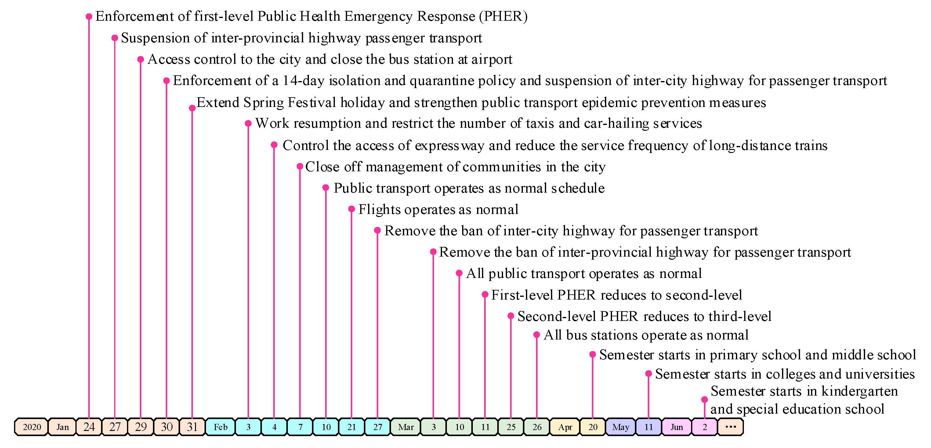
2.3.1. Analysis Based on the COVID-19 Control Policies

In this study, the implementation of COVID-19 control policies was taken as a timeline and the impacts on taxi travel were analyzed according to the timeline. As presented in Figure 2, a timeline diagram of main events was summarized based on the timeline of the epidemic control policies issued by Chongqing municipal government.

2.3.2. Spatial Clustering and Regional Division of POI

The POIs were clustered and mapped onto multiple regions as follows: by following steps:

• Extract the origin and destination (OD) of taxi trips within the study area from the trajectory datasets, and conduct a density-based clustering analysis for calculating their centroid coordinates.
• Construct the Thiessen polygons based on the centroid points determined in step 1, and use the Thiessen polygons as the basic research unit.
• Calculate the number of OD points within each Thiessen polygon. Establish a spatial connection between OD points and polygons, and calculate the amount of OD points within the polygons.
• Calculate the number of POI within each Thiessen polygon for each POI category.
• Propose and construct a model to analyze the driving force of each category of POI on OD.

2.3.3. Spatial Weight Matrix

Normally, three typical spatial weight matrices are used for spatial analysis including spatial adjacency matrix, distance-based geographic weight matrix, and socio-economic distance matrix. The general expression of the spatial weight matrix is shown in Equation (1).

$$\mathrm{w}=\left(\begin{array}{ccc}{\omega }_{11}& \cdots & {\omega }_{1n}\\ ⋮& \ddots & ⋮\\ {\omega }_{n1}& \cdots & {\omega }_{nn}\end{array}\right)$$

(1)

The n by n spatial weight matrix quantifies the spatial correlation between different polygon units that ω_ij represents the spatial correlation between the polygon i and polygon j. In this study, Rook adjacency matrix is selected to determine ω_ij in the spatial weight matrix. The Rook adjacency matrix is expressed in Equation (2):

$${\omega }_{ij}=\{\begin{array}{c}1,\mathrm{if} a_i\mathrm{and} a_j \mathrm{have} \mathrm{a} \mathrm{common} \mathrm{edge}\\ 0, \mathrm{otherwise}\end{array}$$

(2)

where a_i and a_j represent two polygon units in the study area, respectively. As explained in Equation (2), ω_ij equals to 1 if polygon i and polygon j have a common edge and equals to 0 otherwise.

2.3.4. Measurement of Spatial Autocorrelation

Global autocorrelation measurement and local autocorrelation measurement are two typical spatial autocorrelation measurements. In this study, one of the most widely used statistical method global Moran’s I is selected and the expression of global Moran’s I is shown in Equation (3) [48].

$$I=\frac{n}{{{\displaystyle \sum }}_i{{\displaystyle \sum }}_j{\omega }_{ij}}\frac{{{\displaystyle \sum }}_i{{\displaystyle \sum }}_j{\omega }_{ij}\left(x_i-\overline{x}\right)\left(x_j-\overline{x}\right)}{{{\displaystyle \sum }}_i{\left(x_i-\overline{x}\right)}^2}$$

(3)

where n is the number of samples, ω_ij is the (i, j) element of the spatial weight matrix W, x_i and x_j are the observation values of spatial units i and j, and $\overline{x}$. is the mean of observation values. The calculated value of Moran’s I is generally between [−1, 1] and a stronger spatial correlation is reflected by a higher absolute value. The positive value of Moran’s I indicates a positive correlation while negative value reveals a negative correlation. No correlation is indicated if the Moran’s I value equals to 0.

2.3.5. Model Selection

As mentioned in the methodology, the study area has been divided into different independent research units to explore the relationship between POI and taxi travel. Therefore, the influence of spatial effects should be considered by analyzing the differences of travel related characteristics influenced by different spatial factors. Moreover, the spatial distribution of POI is somehow convergent and similar POI may have space aggregation because of the similarity of land use categories [49].

Several spatial econometric models are proposed by previous studies [50]. In this study, the spillover effects of each variable on the same region are analyzed, and influences of the errors of dependent variables in adjacent regions on the observations in the same region are also explored. In this case, spatial error model (SEM) and spatial lag model (SLM) are considered for the model selection. The model selection is conducted by following instruction proposed by Anselin [51], and the steps for spatial measurement model selection are explained as follows:

• Make an Ordinary Least Squares (OLS) estimation.
• Conduct the Lagrange Multiplier test and compare two Lagrange Multiplier statistics Lagrange Multiplier test-spatial error (LMERR) and Lagrange Multiplier test-spatial lag (LMLAG).
• There is no need to perform a spatial measurement model if none of them are statistically significant.
• The spatial measurement model is selected if only one of them is statistically significant.
• Compare the Robust R-LMERR and R-LMLAG if both of them are statistically significant and select the spatial measurement model with more significant statistics.

Two models, namely the spatial error model (SEM) and the spatial lag model (SLM), were used, as presented below.

Spatial error model (SEM) is widely used in many spatial econometric fields, which reflects the spatial dependence effects through the spatial autocorrelation setting of the error term. The expression is as follows:

$$y=X\beta +\mu$$

(4)

$$\mu =\lambda W\mu +\epsilon$$

(5)

$$\epsilon ~N\left(0,{\sigma }^2{I}_n\right)$$

(6)

where y is the dependent variable, X is the independent variable, μ is the regression residual vector, W is the spatial weight matrix, β is the independent variable coefficient, λ is the coefficient of the spatial correlation error, and ε is the random interference term.

The expression of the Lagrange multiplier test for SEM is:

$$L{M}_{\lambda }=\frac{{\left(n{e}^{\prime }We/e^{\prime }e\right)}^2}{tr\left(\left(W+W^{\prime }\right)W\right)}\backsim {\chi }^2\left(1\right)$$

(7)

where e is the residual error obtained by least square estimation of y = Xβ + ε.

By contrast, spatial lag model (SLM) solves the spatial dependence by adding the spatial autocorrelation setting of the dependent variable, and the expression of the model is as follows:

$$y = \rho Wy + X\beta + \epsilon$$

(8)

$$\epsilon ~N\left(0,{\sigma }^2{I}_n\right)$$

(9)

where y is the dependent variable, X is the independent variable, W is the spatial weight matrix, β is the coefficient of the independent variable, ρ is the parameter of the spatial lag term Wy, and ε is the random interference term.

The expression of the Lagrange multiplier test for SLM is:

$$L{M}_{\rho }=\frac{{\left(n{e}^{\prime }Wy/e^{\prime }e\right)}^2}{tr\left(\left(W+W^{\prime }\right)W\right)+n{\left(WX\beta \right)}^{\prime }\left(I_n-X{\left(X^{\prime }X\right)}^{-1}{X}^{\prime }\right)\left(WX\beta \right)/e^{\prime }e}\backsim {\chi }^2$$

(10)

where e is the residual of the least squares estimate.

The results of model selection are discussed in Section 3.2.2.

2.3.6. Variable Selection

In this study, origin and destination of taxi trips are chosen as dependent variables in the model. Meanwhile, seven independent variables are selected associated with seven different categories of POI mentioned in Section 2.2. The number of OD and seven different POI within each polygon unit are measured and the model is further analyzed based on the selected spatial econometric model. The description of each variable is shown in

Table 2. The variables’ description.

Variable Category	Name	Description
Dependent variable	Origins (O)/ Destinations (D)	the number of origins and destinations of taxi trips
Independent variables	Consumption: γ1	the number of Consumption POI within the polygon units
	Business_Government: γ2	the number of Business-Government POI within the polygon units
	Leisure: γ3	the number of Leisure POI within the polygon units
	Medical_Services: γ4	the number of Medical-Services POI within the polygon units
	Residential_Quarter: γ5	the number of Residential-Quarter POI within the polygon units
	Services_Around: γ6	the number of Services-Around POI within the polygon units
	Transportation: γ7	the number of Transportation POI within the polygon units

.

2.4. Social Activities Recovery Level Evaluation Model

2.4.1. Construction of Indicator System

A social activity recovery level evaluation model was proposed and constructed based on the taxi travel datasets indicator system to evaluate the recovery level of urban social activities in the post-epidemic period [52]. All indicators involved in the model are extracted from the taxi datasets and the details of constructed taxi travel datasets indicator system are shown in

Table 3. Evaluation Indicator System of Social Activity Recovery Level.

Index	Indicator Name	Indicator Description and Calculation	Indicator Weights
1	Total trips Ti	Total number of taxi trips in one day	W1
2	Total operating income Ri	Total operating income of taxi in one day	W2
3	Proportion of night trips PNTi	The number of taxi trips from 8 PM to 2 AM in the morning TNi account for the proportion of all-day taxi trips Ti: PNTi = TNi/Ti	W3
4	Proportion of trips from transport hubs PTHi	The number of taxi trips departing from the transport hubs THi account for the proportion of all-day taxi trips Ti: PTHi = THi/Ti	W4
5	Time utilization ratio TURi	Occupy time as a proportion of operating time	W5
6	Mileage ultization rate MURi	Occupy mileage as a proportion of operating mileage	W6
7	Average trip time ATTi	Average travel time of taxi trips on the day	W7
8	Relative trip time of the morning peak RTTi	The ratio of the average taxi trip time during morning peak AMTi to the average trip time on the day ATTi: RTTi = AMTi/ATTi	W8

.

2.4.2. Indicator Description

• Total trips: More total trips are associated with more travel demand, the more frequent social activities in the city, and the higher the social vitality.
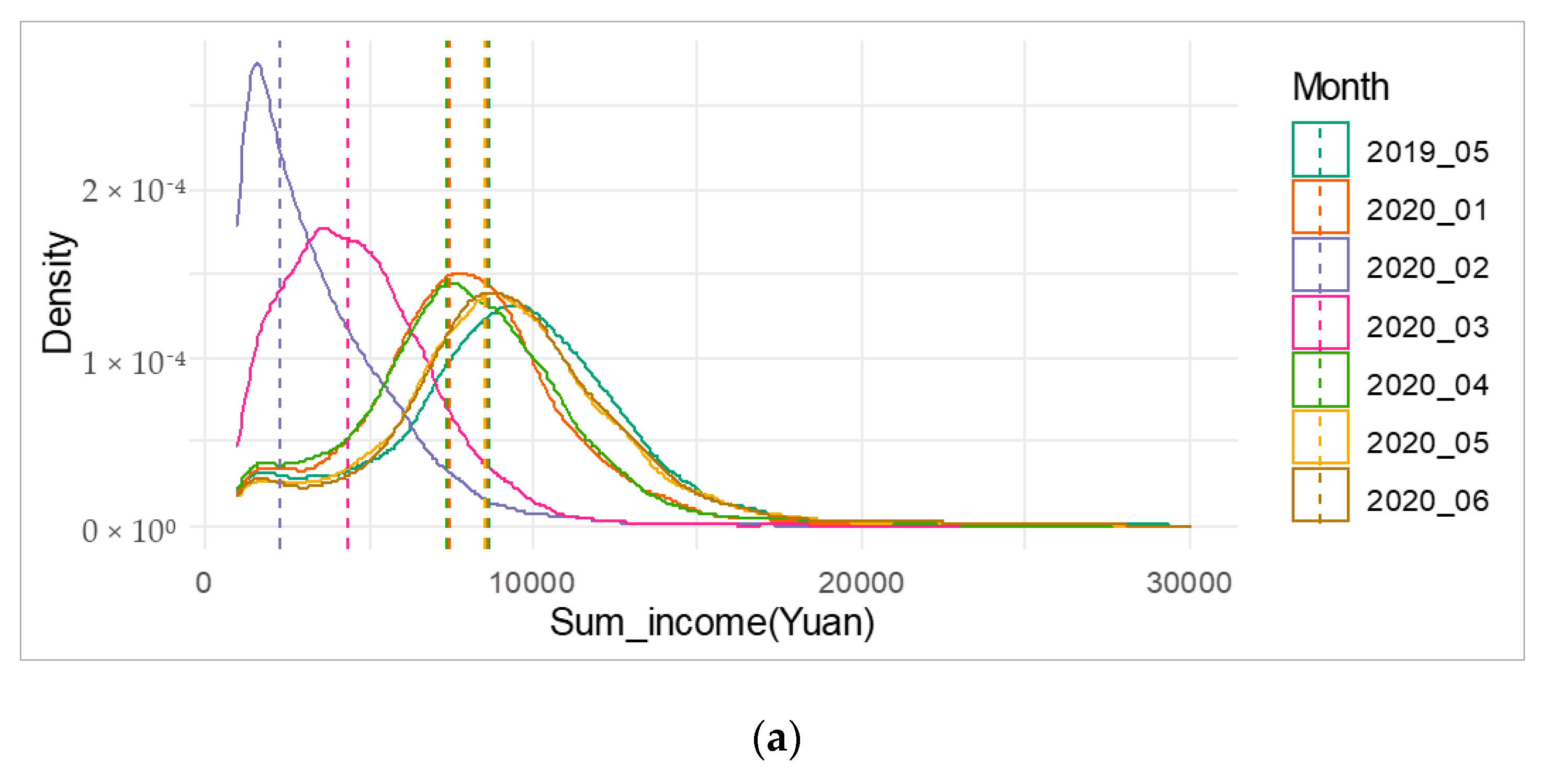
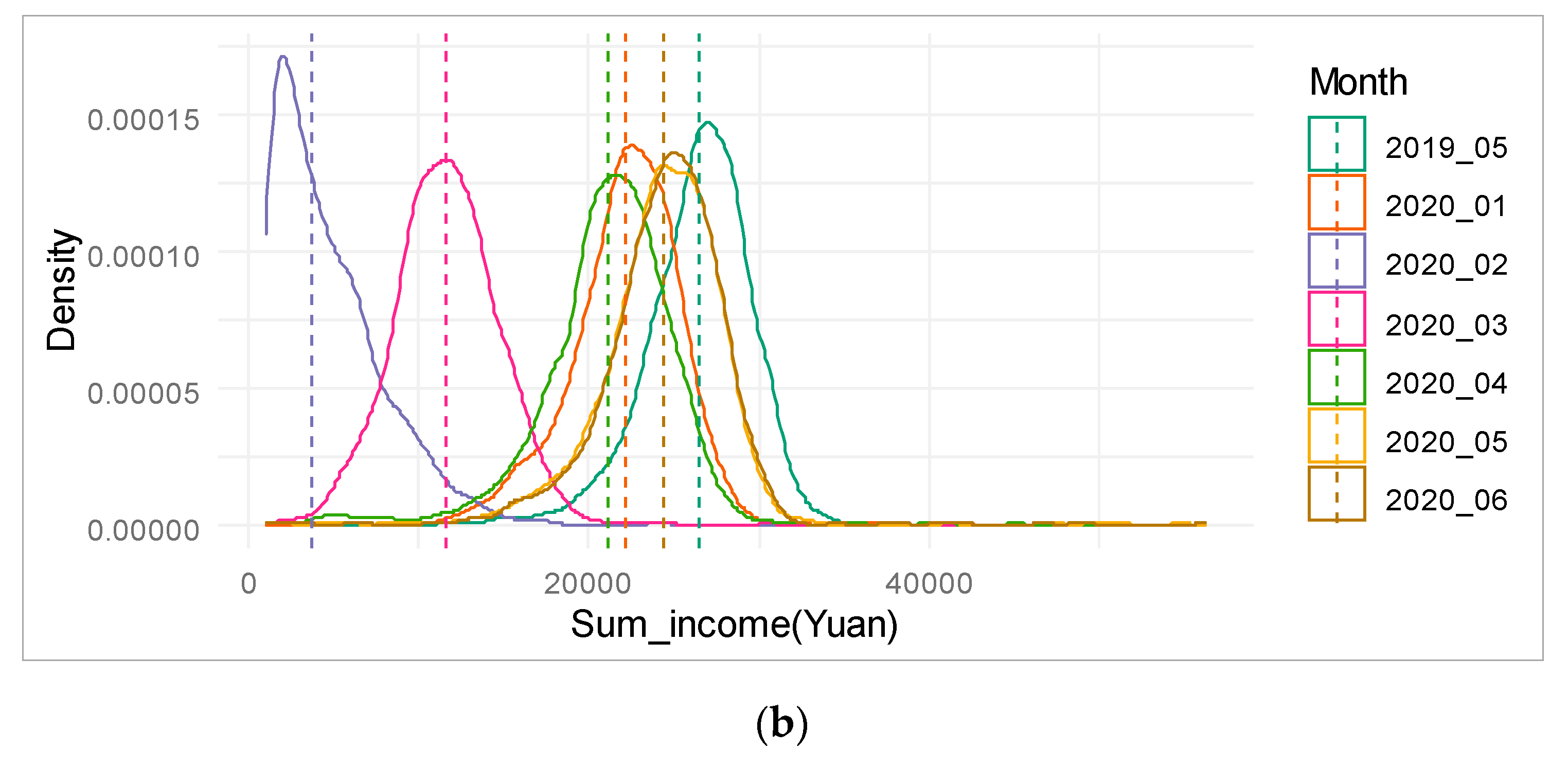
• Total operating income: Higher operating income is associated with more spending on travel and higher the social vitality.
• The proportion of night trips: Night trips refers to the trips between 8 PM and 2 AM. The larger the proportion of night trips, the more prosperous and vibrant city business.
• The proportion of trips from transport hubs: The transport hubs here refer to the city’s railway passenger transport hubs, highway passenger transport hubs, and airports. Generally, the greater the demand for taxi-hailing in transport hubs, the greater the passenger volume of transport hubs the more frequent the city interacts with the outside world, and the higher the social vitality.
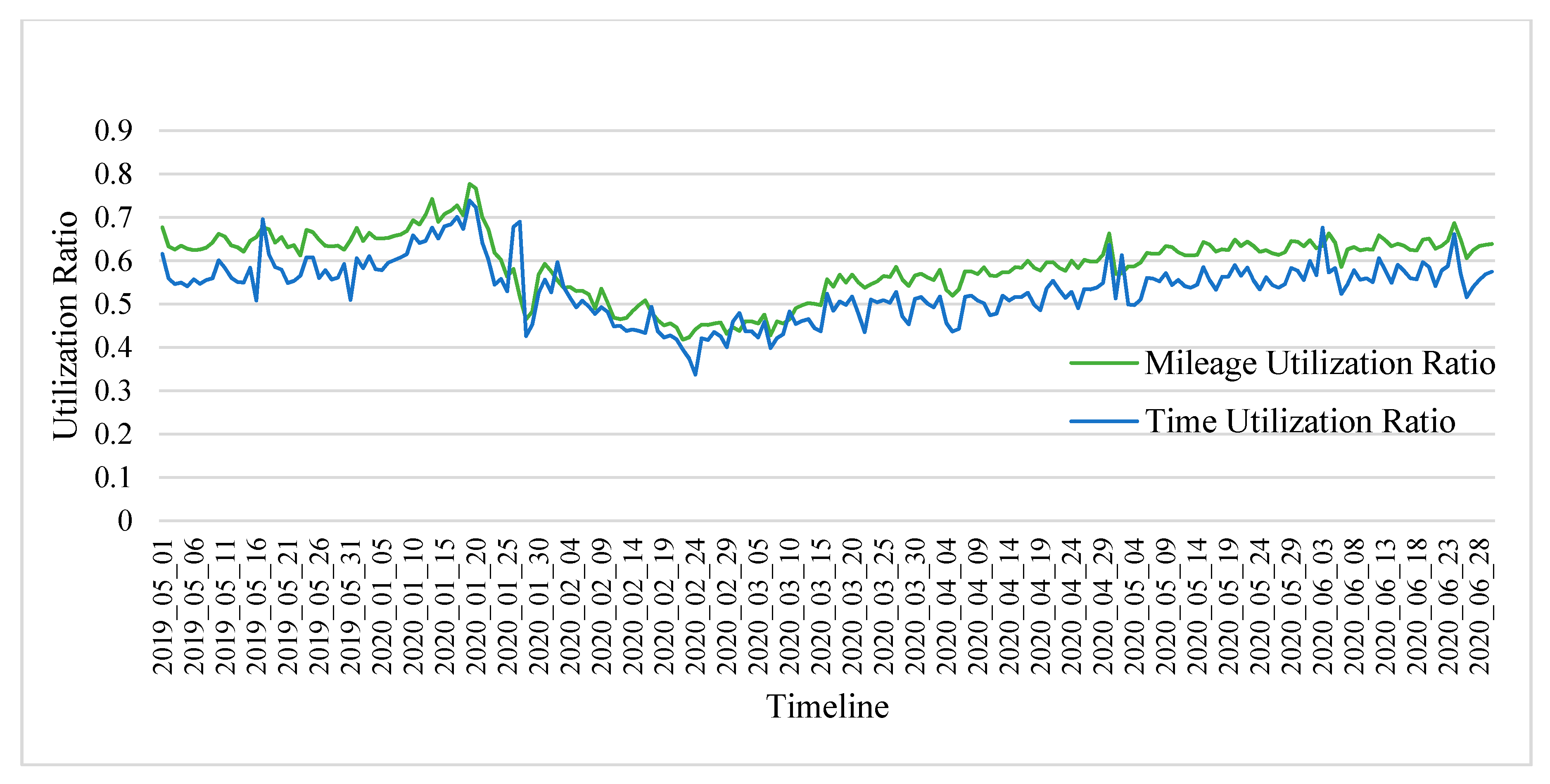
• Time utilization ratio: The higher the time utilization ratio of taxies, the higher the travel demand, and the higher the social vitality.
• Mileage utilization ratio: The higher the mileage utilization ratio of taxies, the higher the travel demand, and the higher the social vitality.
• Average trip time: The longer the travel time for the same trip, the lower the speed and the more saturated the road traffic, the better the recovery of social activities.
• Relative trip time of the morning peak: The morning peak refers to 7:00–9:00 AM of the day. The relative trip time of the morning peak is the ratio of the average travel time during the morning peak to the average travel time of all the trips of the day. The larger the value, the more significant the characteristics of the morning peak, the higher the degree of resumption of work and production, and the better the recovery of social activities.

2.4.3. Recovery Level Assessment Model

The score of each indicator for each characteristic day are calculated and then converted to a 0–1 point by a standardization formula. The total score of each characteristic day is then aggregated by adding each indicator points and a higher total score represents a higher recovery level of social activities during the post-epidemic period. The standardization formula of the indicator score is presented as follows:

$$S_{ij}=\left(V_{ij}-V_{min,j}\right)/\left(V_{max,j}-V_{min,j}\right)$$

(11)

where S_ij represents the calculated score of the j-th indicator on the i-th characteristic day, V_ij represents the original value of j-th indicator on the i-th characteristic day, V_min,j represents the minimum value of the original value of j-th indicator, and V_max,j represents the maximum value of the original value of the j-th indicator. The formula for calculating the total score is shown in Equation (12).

$$T_i=\left(S_{i1}\times W_1+S_{i2}\times W_2+S_{i3}\times W_3+S_{i4}\times W_4+S_{i5}\times W_5+S_{i6}\times W_6+S_{i7}\times W_7+S_{i8}\times W_8\right)\times 100$$

(12)

3. Results and Discussion

3.1. Analyses of Taxi Travel Characteristics before and during the Epidemic

The overall characteristics of the taxi trips in Chongqing are estimated in this section. The numbers of daily taxi trips are compared during the study period and temporal distribution of taxi trips are analyzed among 14 characteristic days. Meanwhile, the distribution of basic information such as trip length, trip time, and trip speed are also discussed in this section. Moreover, taxi mileage utilization ratio is calculated which is the ratio of occupied mileage to total operating mileage, and taxi time utilization ratio is determined which is the ratio of occupied time to total operating time.

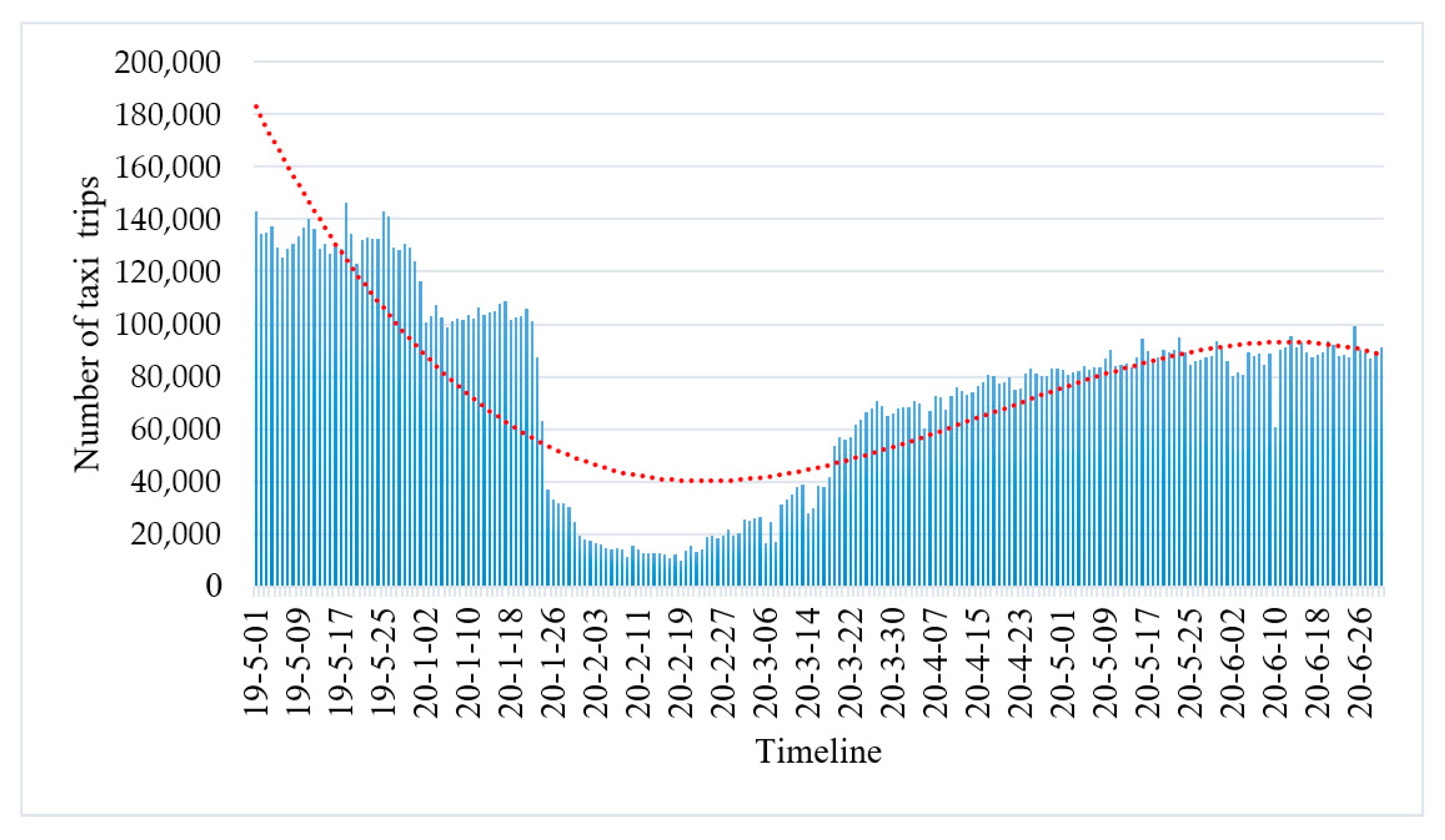
3.1.1. Number of Daily Trips

The number of daily trips during the study period is generated from the datasets as shown in Figure 3. The sample size collected from this particular taxi company accounted for about 35% of the total number of taxies and taxi trips in Chongqing.

As shown in Figure 3, the number of daily taxi trips clearly fluctuated during the study period. During the normal period without any epidemic, the average number of daily taxi trips in Chongqing was 132,756 in May 2019. Due to the outbreak of COVID-19 in January 2020, the number of taxi trips in Chongqing slumped to 63,152 on 24 January with the enforcement of “First-Level Public Health Emergency Response (PHER),” and further dropped to 36,798 on 25 January. During the early stage of the epidemic, the number of daily taxi trips stayed at a low level and reached the lowest value of 12,517 on 14 February. Compared to the normal period without epidemic, the average number of daily taxi trips in February 2020 is 14,975, which is only 11.3% of the average daily taxi trips in May 2019. The number of daily taxi trips started to rise in 11 March because the level of PHER was downgraded by the central government from first level to second level. The daily taxi trips rose gradually from March to June and reached 99,177 on 25 June. Although the daily number of taxi trips kept rising during the post epidemic period, there was still a 30% difference in the number of taxi trips on 25 June compared to the normal period in May 2019.

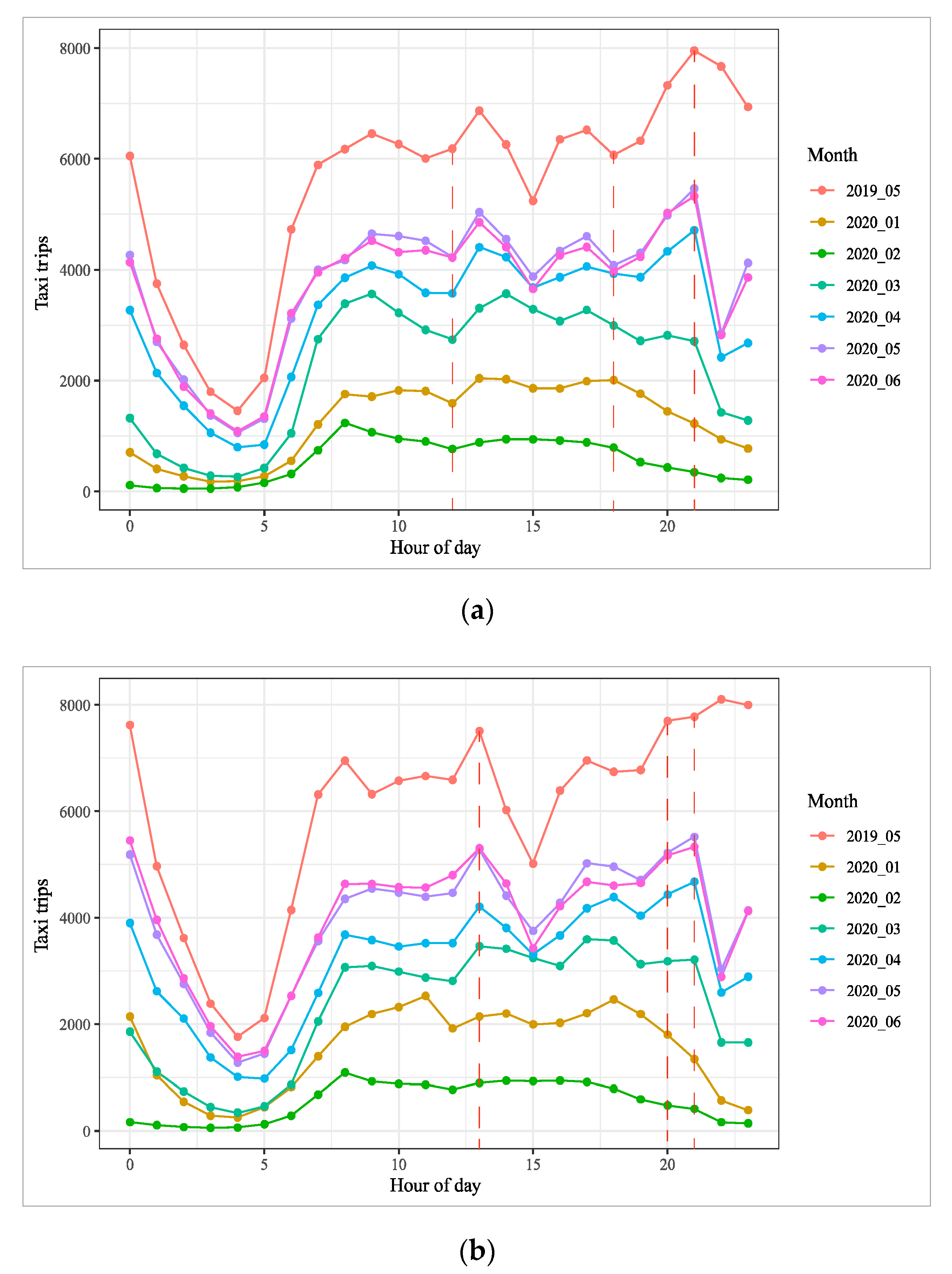
3.1.2. Temporal Distribution of Trips in a Day

In order to explore the temporal distribution of daily trips, a workday and one day of the weekend were selected from the same week for each month. The weather condition is considered because abnormal weather may significantly affect the travel characteristics of taxies [53]. Other disturbances such as holidays, major events, extreme weather conditions (high temperature, low temperature, heavy rainfall, and heavy pollution) were also eliminated during the selection. As a consequence, 14 characteristic days were selected based on the principles mentioned above and the summary of characteristic days are shown in

Table 4. Summary of characteristic days.

Index	Selected Days	Day of the Week	Weather Condition
1	22 May 2019	Wednesday	Cloudy
2	25 May 2019	Saturday	Overcast
3	25 January 2020	Saturday	Overcast
4	29 January 2020	Wednesday	Cloudy
5	20 February 2020	Thursday	Overcast
6	22 February 2020	Saturday	Overcast
7	19 March 2020	Thursday	Cloudy
8	21 March 2020	Saturday	Cloudy
9	11 April 2020	Saturday	Cloudy
10	15 April 2020	Wednesday	Cloudy
11	20 May 2020	Wednesday	Overcast
12	23 May 2020	Saturday	Cloudy
13	13 June 2020	Saturday	Overcast
14	18 June 2020	Thursday	Cloudy

. The temporal distribution of taxi trips on weekdays and weekends are analyzed separately for these characteristic days, as presented in Figure 4.

No significant difference is found between the number of trips on workdays and weekends among the 14 selected characteristic days, while the temporal distribution of taxi trips is slightly different between weekdays and weekends. The differences in temporal distribution between workdays and weekends can be analyzed from the perspective of morning peak, night peak, and epidemic effects.

The morning peak differences are obvious as presented in Figure 4. A relatively gradual rise of taxi trips can be observed during morning peak on weekdays, while a rapid growth occurred on the weekends. Meanwhile, the largest number of taxi trips during the morning peak occurred at 9:00 AM on weekdays but 8:00 AM on weekends.

Moreover, the differences in night trips between the two days in May 2019 are examined. The number of trips began to gradually decrease after 9:00 PM on weekdays and the decreasing amplitude was obvious. However, the number of trips began to gradually decrease after 10:00 PM on weekends while the decreasing amplitude was not obvious, indicating that the vitality of night activities on weekends was higher during normal periods.

Significant differences in temporal distribution of taxi trips can be recognized before and during the epidemic. First, the number of trips dropped sharply during the epidemic period, which has slumped from January, dropped to a minimum in February, gradually recovered from March to May, and maintained at a relatively stable state in June. Secondly, in terms of temporal distribution, the number of trips during the outbreak period is relatively balanced throughout the day, and the overall fluctuation is significantly smaller than the normal period. The most obvious difference before and during the epidemic is at night, where the number of trips gradually rises from around 7:00 PM to around 9:00–10:00 PM during the normal period, and slightly declined until the early morning after reaching the peak with an overall high number of night trips. The number of trips began to decline from around 6:00 PM and reached the lowest point in the early morning during the outbreak period. Thirdly, the characteristics of temporal distribution from March to June after the outbreak period are relatively similar. The number of trips has increased significantly from March especially for night trips, and the trips normally reach a peak point at 9:00 PM and followed by a sharp decrease.

3.1.3. Basic Characteristics of the Trips

As shown in Figure 5, the basic characteristics of taxi trips such as trip length, trip speed, and trip time among 14 characteristic days are summarized by box diagrams. As presented in part (a) and part (b) of Figure 5, little differences can be recognized between workdays and weekends of each month from the perspective of these basic characteristics, indicating similar characteristics of taxi trips between workdays and weekends.

In order to investigate the impacts of epidemic on taxi trips, the distinct characteristics of taxi trips during pre-epidemic period, the outbreak period, and the post-epidemic period were identified and compared. The average trip length during the outbreak period is slightly lower than pre-epidemic period and slightly higher than the post-epidemic period. As expected, the trip speed during the outbreak period is significantly higher than pre-epidemic and post-epidemic periods because of the lower number of vehicles on the streets. As a result, the average trip time during outbreak period is also significantly lower than other periods.

3.1.4. Analysis of Utilization Ratio

The taxi mileage utilization ratio refers to the ratio of occupied mileage to total operating mileage, and taxi time utilization ratio refers to the ratio of occupied time to total operating time. The daily changes of taxi mileage utilization ratio MUR_i and time utilization ratio TUR_i are calculated and shown in Figure 6.

The mileage utilization ratio and time utilization ratio of taxi in Chongqing are significantly influenced by COVID-19. As presented in Figure 6, the mileage utilization ratio and time utilization ratio slightly increased due to the regular Spring Festival travel rush in January 2020, followed by a sharp decline because of the outbreak of the epidemic in February 2020, and then rose gradually over the post epidemic period from March to June 2020.

3.1.5. Monthly Operating Income

The monthly operating income was calculated based on the actual order fare both for drivers and taxies. The kernel density curves are used to reflect the monthly operating income of drivers and taxies are shown in Figure 7.

During the study period, the driver operating income varies significantly from month to month. The driver operating income fell sharply in February, with an average income of about 2200 CNY (China Yuan), which is only about a quarter of the income during normal period (8600 CNY). The average driver operating income in March rose to about 4500 CNY, and rebounded further in the following months. Over the several months of post epidemic period, the driver operating income in May and June are almost the same as the normal period. Interestingly, the driver operating income in January 2020 was marginally affected by the epidemic because the epidemic broke out in late January and the passenger flow during the Spring Festival holiday was relatively larger than normal. The influences caused by the epidemic on taxi monthly operating income are similar to the operating income for drivers, which is also significantly affected by the outbreak of COVID-19.

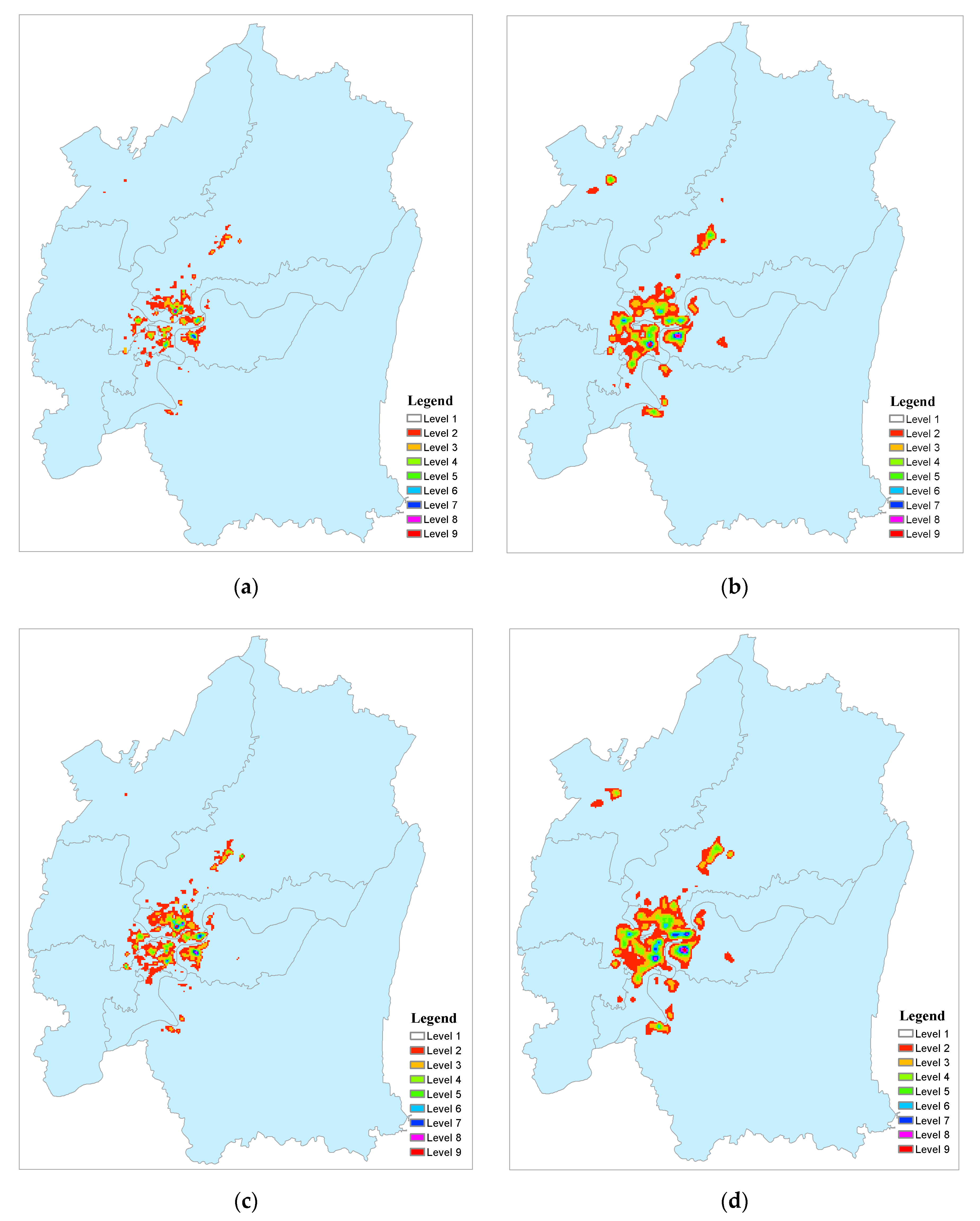
3.1.6. Spatial Distribution of Origins and Destinations

Kernel density estimation are conducted for the comparison of spatial distribution by using data from characteristic days selected in May 2019 and February 2020. The spatial distribution of taxi trips on weekdays are shown by four Kernel density diagrams in Figure 8.

As presented in part (a) and (b) of Figure 8, the spatial distribution of trip origin during the epidemic period and the normal period are significantly different. The range of distribution is larger for the epidemic period than the normal period. Meanwhile, the spatial aggregation is weakened and the differences in travel density within the region are also reduced compared to the normal period. Moreover, changes in the quantity and distribution of travel hot spots can be recognized from the figure.

As presented in part (c) and (d) of Figure 8, the differences in the spatial distribution of trip destination between the epidemic period and the normal period is also obvious. The distribution range of trip destination is also larger for the epidemic period than the normal period and the differences between regions are reduced and relatively balanced for the epidemic period. Meanwhile, some new travel hot spots emerged in the epidemic period in February 2020.

In summary, taxi trips were relatively scattered in spatial distribution during the epidemic period and many concentrated residential areas were transformed from low-travel areas to new travel hotspots due to the epidemic.

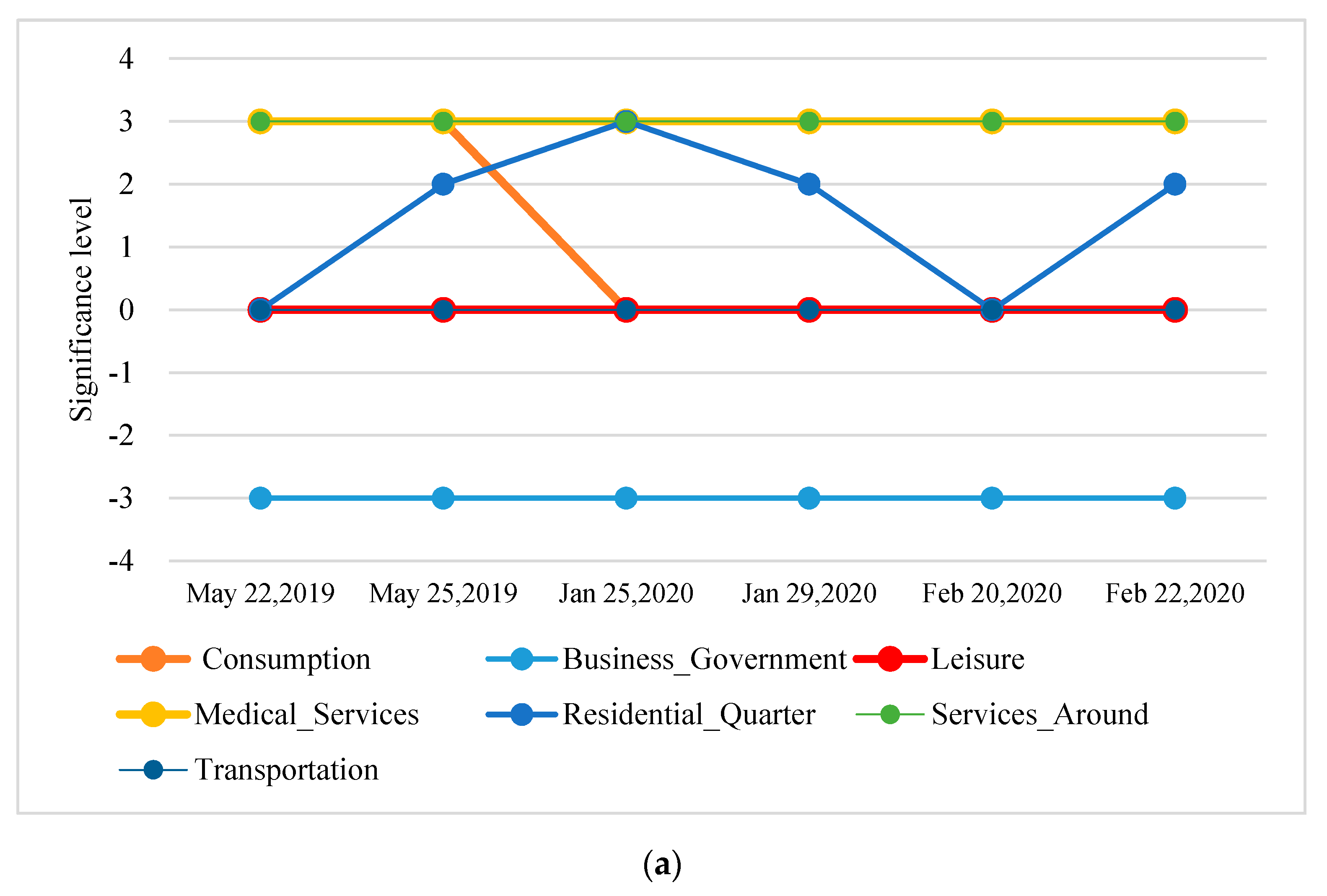
3.2. Analysis of Changes in Travel Driving Force

3.2.1. Results of POI Regional Statistics and Regional Division

An unsupervised learning algorithm is introduced to perform spatial clustering of POI and the research area is divided into 768 units based on the clustering analysis. The results of the division showed that most subject units in the urban inner area are relatively small, while the units in the suburbs are relatively large.

3.2.2. Results of Model Selection

An empirical analysis of taxi travel driving forces was conducted by using the taxi trip data from six characteristic days in three different time periods. The selected characteristic days including 22 and 25 May in 2019 for normal period, 25 and 29 January in 2020 for epidemic period, as well as the 20 and 22 February in 2020 for post epidemic period.

According to the model selection method proposed by Anselin, a spatial OLS regression analysis is conducted on the first characteristic day (22 May 2019). By substituting the spatial weight matrix into the OLS regression, the p-value of the two Lagrange Multiplier statistics LMERR and LMLAG are obtained as 0, indicating that both of the statistics are statistically significant and further efforts are needed for model selection. In this case, the p-values of two robust Lagrange multipliers R-LMLAG and R-LMERR are generated as 0 and 0.351 respectively, which means the R-LMERR statistic is non-significant and thus spatial lag model (SLM) should be selected as the analysis model in this study. Test results by using data from other characteristic days are in accordance with the first characteristic day, which supports the selection of spatial lag model. Moreover, a multicollinearity test was performed on variables by estimating the value of variable inflation factor (VIF). As a result, the largest variable inflation factor is 6.28 and it is smaller than the maximal acceptable value of 10, indicating that no significant multicollinearity problem exists in the model.

3.2.3. Moran’s I Results

Moran’s I for the trip origins and destinations of the research units among six characteristic days were calculated and are shown in Figure 9.

According to the results, the spatial correlation of trip origins and trip destinations on each characteristic day are statistically significant. As presented in Figure 9, the Moran’s I value of origin and destination are all positive during the study period, which means the number of origins and destinations are positively related to the spatial distribution. The largest value of Moran’s I is close to 0.4, and the spatial correlation between trip destination is higher than that of trip origin in most periods, which demonstrates that the spatial correlation between the trip destination is stronger. Both Moran’s I values showed a downward trend after the outbreak of COVID-19 and the spatial correlation is gradually weakened in the following months which means the spatial correlation is further decreased because of the epidemic.

3.2.4. Results of Spatial Lag Model (SLM)

The SLM estimations are carried out to analyze the impact of POI on trip origin and destination among the six characteristic days. The SLM estimation results are listed in

Table 5. Results of spatial lag model (SLM) on trip origins.

	Name	Variable	Coefficient	Std.Error	z.Value	p-Value
Date
22 May 2019		W_ori190522	0.590	0.035	16.652	0.000
		CONSTANT	−14.621	9.747	−1.500	0.134
		γ1	0.226	0.053	4.269	0.000
		γ2	−0.511	0.128	−3.994	0.000
		γ3	0.018	0.295	0.061	0.951
		γ4	3.367	0.719	4.682	0.000
		γ5	0.202	0.144	1.407	0.159
		γ6	0.740	0.101	7.335	0.000
		γ7	0.044	0.095	0.467	0.641
25 May 2019		W_ori190525	0.599	0.035	17.197	0.000
		CONSTANT	−19.550	10.136	−1.929	0.054
		γ1	0.298	0.055	5.393	0.000
		γ2	−0.533	0.133	−4.005	0.000
		γ3	0.235	0.306	0.768	0.443
		γ4	3.197	0.747	4.282	0.000
		γ5	0.318	0.149	2.127	0.033
		γ6	0.647	0.105	6.184	0.000
		γ7	0.030	0.098	0.304	0.761
25 January 2020		W_ori20200125	0.573	0.036	15.748	0.000
		CONSTANT	−4.360	2.885	−1.511	0.131
		γ1	0.011	0.016	0.687	0.492
		γ2	−0.131	0.038	−3.485	0.000
		γ3	−0.061	0.088	−0.699	0.484
		γ4	1.674	0.215	7.785	0.000
		γ5	0.150	0.043	3.496	0.000
		γ6	0.221	0.030	7.344	0.000
		γ7	0.010	0.028	0.364	0.716
29 January 2020		W_ori20200129	0.526	0.039	13.547	0.000
		CONSTANT	−0.150	2.480	−0.060	0.952
		γ1	−0.001	0.014	−0.087	0.930
		γ2	−0.131	0.032	−4.056	0.000
		γ3	−0.071	0.075	−0.942	0.346
		γ4	1.525	0.184	8.269	0.000
		γ5	0.086	0.037	2.335	0.020
		γ6	0.198	0.026	7.674	0.000
		γ7	−0.006	0.024	−0.252	0.801
20 February 2020		W_ori20200220	0.509	0.040	12.719	0.000
		CONSTANT	0.281	1.303	0.215	0.829
		γ1	0.003	0.007	0.385	0.700
		γ2	−0.062	0.017	−3.602	0.000
		γ3	−0.021	0.040	−0.533	0.594
		γ4	0.922	0.098	9.368	0.000
		γ5	0.024	0.020	1.220	0.223
		γ6	0.079	0.014	5.746	0.000
		γ7	−0.012	0.013	−0.966	0.334
22 February 2020		W_ori20200222	0.479	0.041	11.656	0.000
		CONSTANT	−0.216	1.241	−0.174	0.862
		γ1	0.006	0.007	0.928	0.353
		γ2	−0.062	0.016	−3.811	0.000
		γ3	−0.035	0.038	−0.904	0.366
		γ4	0.786	0.094	8.408	0.000
		γ5	0.047	0.019	2.517	0.012
		γ6	0.081	0.013	6.204	0.000
		γ7	−0.007	0.012	−0.585	0.558

;

Table 6. Results of SLM on trip destinations.

	Name	Variable	Coefficient	Std.Error	z.value	p-Value
Date
22 May 2019		W_des190522	0.636	0.033	19.119	0.000
		CONSTANT	−10.014	8.516	−1.176	0.240
		γ1	0.081	0.045	1.804	0.071
		γ2	−0.446	0.109	−4.098	0.000
		γ3	−0.008	0.251	−0.031	0.975
		γ4	3.241	0.614	5.281	0.000
		γ5	0.384	0.123	3.128	0.002
		γ6	0.683	0.086	7.919	0.000
		γ7	0.072	0.081	0.893	0.372
25 May 2019		W_des190525	0.633	0.033	19.084	0.000
		CONSTANT	−14.554	8.950	−1.626	0.104
		γ1	0.166	0.047	3.512	0.000
		γ2	−0.458	0.114	−4.011	0.000
		γ3	0.115	0.262	0.437	0.662
		γ4	2.804	0.641	4.376	0.000
		γ5	0.466	0.128	3.633	0.000
		γ6	0.639	0.090	7.108	0.000
		γ7	0.073	0.084	0.868	0.385
25 January 2020		W_des20200125	0.565	0.037	15.150	0.000
		CONSTANT	−1.387	2.868	−0.484	0.629
		γ1	−0.015	0.015	−0.941	0.347
		γ2	−0.101	0.037	−2.767	0.006
		γ3	−0.041	0.086	−0.479	0.632
		γ4	1.464	0.211	6.948	0.000
		γ5	0.191	0.042	4.535	0.000
		γ6	0.222	0.030	7.511	0.000
		γ7	0.002	0.028	0.060	0.952
29 January 2020		W_des20200129	0.560	0.037	15.303	0.000
		CONSTANT	−0.041	2.175	−0.019	0.985
		γ1	−0.015	0.012	−1.267	0.205
		γ2	−0.106	0.027	−3.860	0.000
		γ3	−0.065	0.064	−1.014	0.310
		γ4	1.480	0.158	9.384	0.000
		γ5	0.139	0.031	4.422	0.000
		γ6	0.165	0.022	7.462	0.000
		γ7	−0.011	0.021	−0.526	0.599
20 February 2020		W_des20200220	0.543	0.038	14.205	0.000
		CONSTANT	0.872	1.158	0.753	0.452
		γ1	−0.013	0.006	−2.094	0.036
		γ2	−0.054	0.015	−3.649	0.000
		γ3	0.000	0.035	−0.002	0.998
		γ4	0.808	0.085	9.511	0.000
		γ5	0.053	0.017	3.158	0.002
		γ6	0.076	0.012	6.385	0.000
		γ7	−0.006	0.011	−0.529	0.597
22 February 2020		W_des20200222	0.533	0.039	13.737	0.000
		CONSTANT	0.586	1.087	0.539	0.590
		γ1	−0.009	0.006	−1.475	0.140
		γ2	−0.045	0.014	−3.280	0.001
		γ3	−0.025	0.032	−0.765	0.444
		γ4	0.660	0.080	8.297	0.000
		γ5	0.072	0.016	4.551	0.000
		γ6	0.070	0.011	6.279	0.000
		γ7	−0.004	0.010	−0.391	0.696

which includes the estimated coefficients of variables and their corresponding standard errors, asymptotic t-tests (z statistics), and p-values. The estimated variables for each characteristic day include the spatial lag independent variables, which are generated from the spatial lag model and the name of spatial lag independent variables are started with “W_” as shown in the Table. The constant value and other 7 independent variables associated with 7 categories of POI are also generated by the SLM estimation.

Obvious differences in the model coefficients and significance can be observed during the different characteristic days. The spatial lag coefficients are statistically significant on weekdays and weekends, indicating the significant spatial lag effects in the model which can further verify the accuracy of the model selection. To explore the impacts of POI on taxi travel at each period, the significance level of each POI related variable was evaluated and shown in Figure 10, as well as the sign of its corresponding coefficient.

Over the study period, only the impacts of Consumption γ₁ and Residential_Quarter γ₅ on the distribution of taxi origin and destination have significantly changed during the epidemic period. More specifically, the impact of Consumption γ₁ on trip origin has changed from a positive correlation at significance level of 1% to insignificant due to the epidemic. Meanwhile, the impact of Consumption γ₁ on trip destination has changed from a positive correlation at significance level of 1% to a negative correlation at significance level of 5% because of the outbreak of the epidemic. On the other hand, the impact of Residential_Quarter γ₅ on trip origin has changed from a positive correlation at 5% significance level to a positive correlation at 1% significance level during the epidemic period. The significance level of the impact of other variables such as Business_Government γ₂, Leisure γ₃, Medical_Services γ₄, Services_Around γ₆ and Transportation γ₇ POI on trip origin and destination has not changed over the study period. As shown in Figure 10, Medical_Services γ₄ and Services_Around γ₆ POI always have positive correlation at the significance level of 1% during the study period, while Leisure γ₃ and Transportation γ₇ have no significant correlation, and Business_Government γ₂ has a negative correlation at 1% significance level.

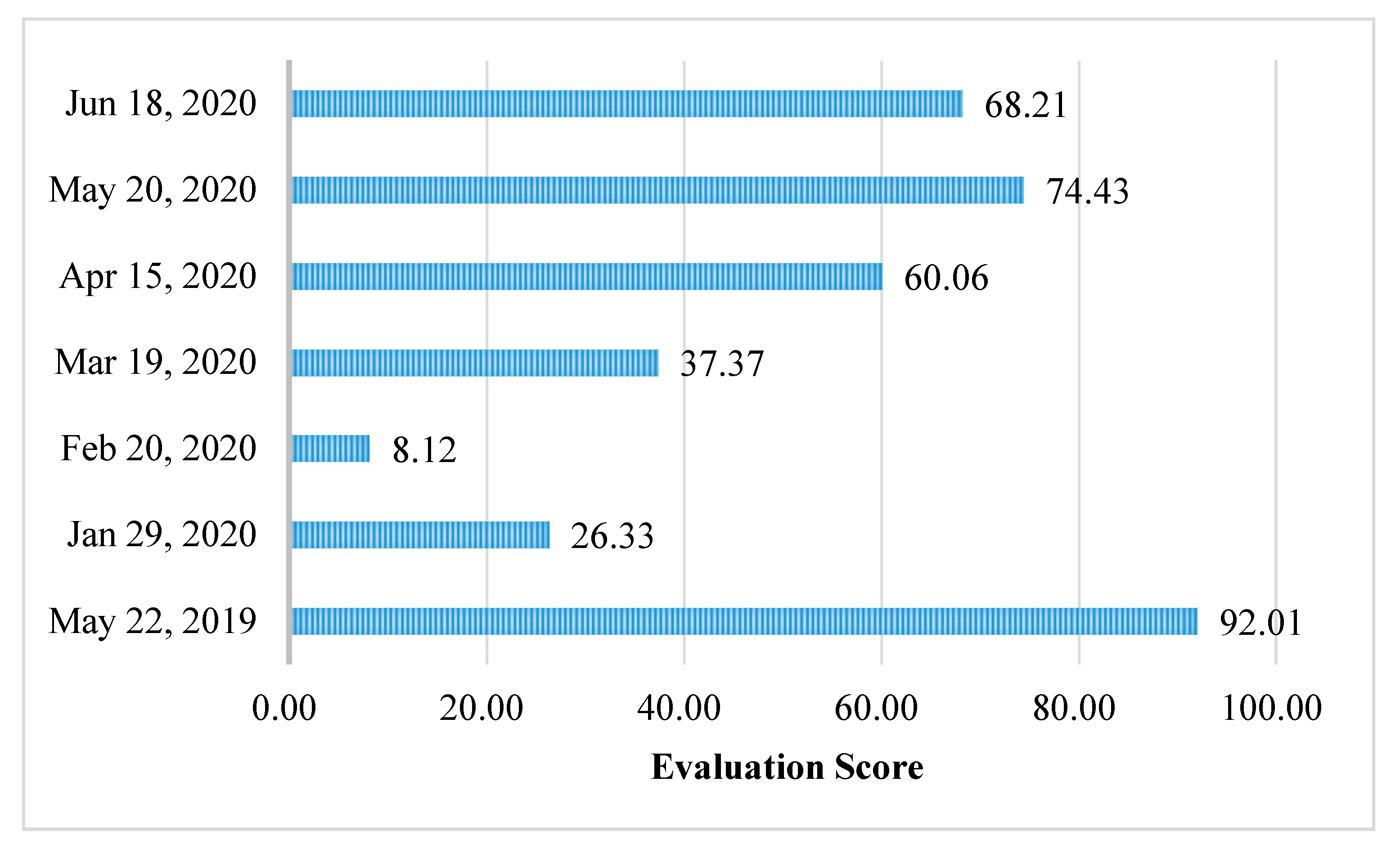
3.3. Assessment of the Recovery Level of Social Activities in the Post-Epidemic Period

The weight of each indicator in the recovery level assessment model are obtained based on the expert scoring method, and then put the weight of each indicator into Equation (12) to get the new calculation formula:

$$T_i=\left(S_{i1}\times 0.28+S_{i2}\times 0.07+S_{i3}\times 0.17+S_{i4}\times 0.12+S_{i5}\times 0.13+S_{i6}\times 0.13+S_{i7}\times 0.05+S_{i8}\times 0.05\right)\times 100$$

(13)

The total score of each characteristic day is calculated and shown in Figure 11. The total score of May 2019 in the normal period is calculated as 92.01. As presented in Figure 11, it is obvious that February has the lowest total score (8.12) over the study period because it has the lowest intensity of social activities due to the outbreak of the epidemic. The social activities began to recover in March (37.37), but still at a relatively low level compared to the normal period. The recovery level of social activities increased significantly in the following two months and reached the highest level during the post epidemic period in May with the total score of 74.43. A slight decrease of score occurred in June (68.21) because of the typical rainy season in Chongqing, coupled with the abnormal long duration of rainy in the year which may affect the taxi travel and lead to a reduction of social activities.

4. Conclusions

This paper analyzes the impact of COVID-19 on social activities and travel behavior of people from the perspective of taxi travel in Chongqing China. As expected, the impacts of the epidemic on urban mobility and trip distribution is significant and obvious which is reflected in several aspects. The total number of taxi trips had a sharp decline during the epidemic period and the characteristics of taxi trips have also changed significantly due to the strict epidemic control policies. The results of the spatial lag model based on taxi trips and POI demonstrated that the driving factors of taxi travel have changed significantly during the epidemic period, and the impact of different types of POI on taxi travel is quite different compared to the normal period. The assessment results of social activity recovery level revealed that social activities in Chongqing were significantly influenced by the epidemic since February 2020, but social vitality has gradually recovered in the following months due to the work resumption and mitigation of epidemic control policies in the post epidemic period. The main findings and conclusions are summarized as follows:

Obvious differences can be found between the number of trips during epidemic period and normal period. The average daily taxi trips in February 2020 were only 11.3% of May 2019. Taxi trips began to rise gradually in March, and reached about 70.0% of the normal period in June 2020. The peak hours of taxi trips are not salient that the daytime trips are relatively stable while the nighttime trips (9:00 PM–5:00 AM) are extremely low during the epidemic period. The proportion of nighttime trips on weekdays in May 2019 and January to June 2020 were 28.8%, 15.4%, 8.5%, 15.7%, 24.4%, 26.4%, and 26.7% respectively and the nighttime trips on weekdays from January to June 2020 were 12.3%, 3.0%, 22.0%, 48.7%, 62.3%, and 60.9% of the nighttime trips during the normal period.

The change of taxi travel characteristics was analyzed from the perspective of travel time, travel speed, travel distance, and spatial distribution. The average travel time, average travel speed, and average distance of taxi trips in February 2020 have decreased by 22.6%, increased by 29.4%, and increased by 2.4% respectively compared to the data in May 2019. The trip distance has not changed obviously, but the travel speed has increased significantly due to the reduction of traffic volume during the epidemic period. The mileage utilization rate and time utilization rate of taxies in February 2020 decreased by 24.6% and 20.3% respectively compared to May 2019. The average monthly income of drivers and taxies was the lowest in February 2020 with 2261.0 CNY and 3754.5 CNY respectively, which were only 26.1% and 14.2% of the average monthly income in May 2019. However, the average monthly income of drivers and taxies has risen to 98.6% and 91.9% of the normal period respectively in May 2020. Although the total number of trips decreased significantly, the income of drivers and taxies has not been significantly influenced because of the reduction of taxi supply in the city. The distribution of origins and destinations of taxi travel is relatively scattered in space, and some areas with fewer taxi trips have become hot spots during the epidemic period.

The change of taxi travel’s driving force was estimated by SLM model. Moran’s I between trip origins and Moran’s I between trip destinations showed a downward trend after the outbreak of the epidemic, which indicates that the spatial correlation between regions is becoming smaller and smaller. The results of the spatial lag model demonstrated that the impact of Consumption POI on taxi travel is significantly decreased and the impact of Residential_Quarter POI on taxi travel significantly increased during the epidemic period. It also revealed that the unnecessary travel for residential purpose has been greatly reduced during the epidemic period, while the necessary travel for life purpose occupied a dominant position.

The evaluation of social activity recovery level was conducted and realized that the evaluation score is only 8.12 in February 2020, which is 8.8% of 92.01 in May 2019. The assessment score started to rise from March and reached 74.43 in May 2020, followed by a marginal decline in June to 68.21. The main reason for the decline is the impact of the rainy season in June, which could affect the corresponding evaluation indicators, and further lead to the decline of the total evaluation score.

Although some research work has been done on the interaction between COVID-19 and taxi trips, there are still several limitations in this study. First of all, only taxi trips and taxi related datasets are included in this study without any other transport mode in the city. Secondly, the microscopic study on the spatial-temporal evolution characteristics of travel has not been conducted such as the study of travel spatial-temporal changes in a specific time or specific areas. Moreover, no further study on travel trajectories and OD flow direction of trips are conducted, which would help to explore the correlation between travel behavior, POI, and urban spatial structure during the epidemic period. Deviation and bias may also occur during the evaluation of social activity recovery level because only taxi travel data are included in the model. Therefore, it is more reliable to involve data from other mobility options in the model for deviation minimization.

In the future, several relevant research areas could be conducted in this direction by solving the limitations of this study. First of all, public transport datasets and private car datasets can be included to explore the impacts of COVID-19 on travel behavior from a more comprehensive perspective. Meanwhile, the data of travel trajectories and traffic flow can be utilized to analyze the spatial-temporal characteristics of travel behavior during the epidemic period from a microcosmic aspect. At the same time, the intrinsic mechanism between urban space, traffic usage, and epidemic spread could be estimated based on POI data and urban built-up environment [54]. Furthermore, the further modification of the social activity recovery level model should be explored to improve its accuracy and reliability. In addition, the analysis of the differences of the relationship between the monthly income and working hours of taxi drivers during the epidemic period could be evaluated, and other research such as the impacts of COVID-19 on the psychology of drivers or labor supply elasticity should also be considered to carry out immediately. Although COVID-19 is a potential threat to the urban public transport system, it is also an opportunity for scholars to explore the typical solutions for transport systems during the epidemic period [55]. Hopefully, sustainable and resilient urban transport systems could be built around the world by more and more excellent studies in this direction to have the capability of resisting other epidemics like COVID-19.

References

1. Leung, K.; Wu, J.T.; Liu, D.; Leung, G.M. First-wave COVID-19 transmissibility and severity in China outside Hubei after control measures, and second-wave scenario planning: A modelling impact assessment. Lancet 2020, 395, 1382–1393. [Google Scholar] [CrossRef]
2. Chakraborty, I.; Maity, P. COVID-19 outbreak: Migration, effects on society, global environment and prevention. Sci. Total Environ. 2020, 728, 138882. [Google Scholar] [CrossRef] [PubMed]
3. Lau, H.; Khosrawipour, V.; Kocbach, P.; Mikolajczyk, A.; Schubert, J.; Bania, J.; Khosrawipour, T. The positive impact of lockdown in Wuhan on containing the COVID-19 outbreak in China. J. Travel Med. 2020, 27, 1–7. [Google Scholar] [CrossRef] [PubMed] [Green Version]
4. Hadjidemetriou, G.M.; Sasidharan, M.; Kouyialis, G.; Parlikad, A.K. The impact of government measures and human mobility trend on COVID-19 related deaths in the UK. Transp. Res. Interdiscip. Perspect. 2020, 6, 100167. [Google Scholar] [CrossRef]
5. Verheyden, B.; Askitas, N.; Tatsiramos, K. Lockdown Strategies, Mobility Patterns and COVID-19. Available online: https://arxiv.org/abs/2006.00531 (accessed on 31 May 2020).
6. Baker, S.R.; Farrokhnia, R.A.; Meyer, S.; Pagel, M.; Yannelis, C. How Does Household Spending Respond to an Epidemic? Consumption during the 2020 COVID-19 Pandemic. Available online: https://www.nber.org/papers/w26949 (accessed on 13 April 2020).
7. World Health Organization. Coronavirus Disease 2019 (COVID-19) Situation Report-72 HIGHLIGHTS; WHO: Geneva, Switzerland, 2020. [Google Scholar]
8. Lipsitch, M.; Cohen, T.; Cooper, B.; Robins, J.M.; Ma, S.; James, L.; Gopalakrishna, G.; Chew, S.K.; Tan, C.C.; Samore, M.H.; et al. Transmission dynamics and control of severe acute respiratory syndrome. Science 2003, 300, 1966–1970. [Google Scholar] [CrossRef] [Green Version]
9. Chinazzi, M.; Davis, J.T.; Ajelli, M.; Gioannini, C.; Litvinova, M.; Merler, S.; Pastore y Piontti, A.; Mu, K.; Rossi, L.; Sun, K.; et al. The effect of travel restrictions on the spread of the 2019 novel coronavirus (COVID-19) outbreak. Science 2020, 368, 395–400. [Google Scholar] [CrossRef] [Green Version]
10. Wilder-Smith, A.; Chiew, C.J.; Lee, V.J. Can we contain the COVID-19 outbreak with the same measures as for SARS? Lancet Infect. Dis. 2020, 20, e102–e107. [Google Scholar] [CrossRef] [Green Version]
11. Kraemer, M.U.G.; Yang, C.-H.; Gutierrez, B.; Wu, C.-H.; Klein, B.; Pigott, D.M.; du Plessis, L.; Faria, N.R.; Li, R.; Hanage, W.P.; et al. The effect of human mobility and control measures on the COVID-19 epidemic in China. Science 2020, 368, 493–497. [Google Scholar] [CrossRef] [Green Version]
12. Tian, H.; Liu, Y.; Li, Y.; Wu, C.H.; Chen, B.; Kraemer, M.U.G.; Li, B.; Cai, J.; Xu, B.; Yang, Q.; et al. An investigation of transmission control measures during the first 50 days of the COVID-19 epidemic in China. Science 2020, 368, 638–642. [Google Scholar] [CrossRef] [Green Version]
13. Zhao, S.; Chen, H. Modeling the epidemic dynamics and control of COVID-19 outbreak in China. Quant. Biol. 2020, 8, 11–19. [Google Scholar] [CrossRef] [Green Version]
14. Wilder-Smith, A.; Freedman, D.O. Isolation, quarantine, social distancing and community containment: Pivotal role for old-style public health measures in the novel coronavirus (2019-nCoV) outbreak. J. Travel Med. 2020, 27, taaa020. [Google Scholar] [CrossRef] [PubMed]
15. Svoboda, T.; Henry, B.; Shulman, L.; Kennedy, E.; Rea, E.; Ng, W.; Wallington, T.; Yaffe, B.; Gournis, E.; Vicencio, E.; et al. Public health measures to control the spread of the severe acute respiratory syndrome during the outbreak in Toronto. N. Engl. J. Med. 2004, 350, 2352–2361. [Google Scholar] [CrossRef] [PubMed]
16. Gumel, A.B.; Ruan, S.; Day, T.; Watmough, J.; Brauer, F.; Van Den Driessche, P.; Gabrielson, D.; Bowman, C.; Alexander, M.E.; Ardal, S.; et al. Modelling strategies for controlling SARS outbreaks. Proc. R. Soc. B Biol. Sci. 2004, 271, 2223–2232. [Google Scholar] [CrossRef] [PubMed]
17. Yen, M.Y.; Schwartz, J.; Chen, S.Y.; King, C.C.; Yang, G.Y.; Hsueh, P.R. Interrupting COVID-19 transmission by implementing enhanced traffic control bundling: Implications for global prevention and control efforts. J. Microbiol. Immunol. Infect. 2020, 53, 377–380. [Google Scholar] [CrossRef]
18. Primc, K.; Slabe-Erker, R. The success of public health measures in Europe during the COVID-19 pandemic. Sustainability 2020, 12, 4321. [Google Scholar] [CrossRef]
19. The Passenger Volume of the 2020 Spring Festival Travel Rush is Significantly Lower than that of Last Year. Available online: http://www.rmjtxw.com/news/yaowen/102949.html (accessed on 20 February 2020).
20. Ministry of Transport of the People’s Republic of China Statistics of Total Passenger Traffic in Central Cities. Available online: http://www.mot.gov.cn/tongjishuju/ (accessed on 26 June 2020).
21. Aloi, A.; Alonso, B.; Benavente, J.; Cordera, R.; Echániz, E.; González, F.; Ladisa, C.; Lezama-Romanelli, R.; López-Parra, Á.; Mazzei, V.; et al. Effects of the COVID-19 lockdown on urban mobility: Empirical evidence from the city of Santander (Spain). Sustainability 2020, 12, 3870. [Google Scholar] [CrossRef]
22. Chen, K.; Wang, M.; Huang, C.; Kinney, P.L.; Anastas, P.T. Air pollution reduction and mortality benefit during the COVID-19 outbreak in China. Lancet Planet. Health 2020, 4, e210–e212. [Google Scholar] [CrossRef]
23. Huang, J.; Wang, H.; Fan, M.; Zhuo, A.; Sun, Y.; Li, Y. Understanding the Impact of the COVID-19 Pandemic on Transportation-related Behaviors with Human Mobility Data. In Proceedings of the 26th ACM SIGKDD Conference on Knowledge Discovery and Data Mining (KDD’20), Virtual Event, New York, NY, USA, 23–27 August 2020; pp. 3443–3450. [Google Scholar]
24. Dubey, A.; Wilbur, M.; Ayman, A.; Ouyang, A.; Poon, V.; Kabir, R.; Vadali, A.; Pugliese, P.; Freudberg, D.; Laszka, A. Impact of COVID-19 on Public Transit Accessibility and Ridership. Available online: https://arxiv.org/abs/2008.02413 (accessed on 6 August 2020).
25. Arellana, J.; Márquez, L.; Cantillo, V. COVID-19 Outbreak in Colombia: An Analysis of Its Impacts on Transport Systems. J. Adv. Transp. 2020, 2020, 8867316. [Google Scholar] [CrossRef]
26. Molloy, J.; Tchervenkov, C.; Schatzmann, T.; Schoeman, B.; Hitermann, B.; Axhausen, K.W. MOBIS-COVID19/13: Results as of 06/07/2020 (Post-Lockdown); Arbeitsbericht Verkehrs und Raumplanung: Zurich, Switzerland, 2020. [Google Scholar]
27. Tirachini, A.; Cats, O. COVID-19 and public transportation: Current assessment, prospects, and research needs. J. Public Transp. 2020, 22, 1–34. [Google Scholar] [CrossRef]
28. Fernandes, N. Economic Effects of Coronavirus Outbreak (COVID-19) on the World Economy. Available online: https://ssrn.com/abstract=3557504 (accessed on 13 April 2020).
29. Batty, M. The Coronavirus crisis: What will the post-pandemic city look like? Environ. Plan. B Urban Anal. City Sci. 2020, 47, 547–552. [Google Scholar] [CrossRef]
30. Tang, J.; Heinimann, H.R.; Han, K. A Bayesian network approach for assessing the general resilience of road transportation systems: A systems perspective. In Proceedings of the CICTP 2019: Transportation in China—Connecting the World, Jiangsu, China, 6–8 June 2019. [Google Scholar]
31. Amekudzi-Kennedy, A.; Labi, S.; Woodall, B.; Chester, M.; Singh, P. Reflections on Pandemics, Civil Infrastructure and Sustainable Development: Five Lessons from COVID-19 through the Lens of Transportation. Available online: https://www.preprints.org/manuscript/202004.0047/v1 (accessed on 6 April 2020).
32. Wang, X.; Miao, S.; Tang, J. Vulnerability and resilience analysis of the air traffic control sector network in China. Sustainability 2020, 12, 3749. [Google Scholar] [CrossRef]
33. Huang, J.; Wang, H.; Xiong, H.; Fan, M.; Zhuo, A.; Li, Y.; Dou, D. Quantifying the Economic Impact of COVID-19 in Mainland China Using Human Mobility Data. Available online: https://arxiv.org/abs/2005.03010 (accessed on 6 May 2020).
34. Gössling, S.; Scott, D.; Hall, C.M. Pandemics, tourism and global change: A rapid assessment of COVID-19. J. Sustain. Tour. 2020, 1–20. [Google Scholar] [CrossRef]
35. Dang, H.A.; Giang, L. Turning Vietnam’s COVID-19 Success into Economic Recovery: A Job-Focused Analysis of Individual Assessments on Their Finance and the Economy. Available online: https://papers.ssrn.com/sol3/papers.cfm?abstract_id=3620630 (accessed on 9 June 2020).
36. Sun, D.; Ding, X. Spatiotemporal evolution of ridesourcing markets under the new restriction policy: A case study in Shanghai. Transp. Res. Part A Policy Pract. 2019, 130, 227–239. [Google Scholar] [CrossRef]
37. Sun, D.; Zhang, K.; Shen, S. Analyzing spatiotemporal traffic line source emissions based on massive didi online car-hailing service data. Transp. Res. Part D Transp. Environ. 2018, 62, 699–714. [Google Scholar] [CrossRef]
38. Gong, L.; Liu, X.; Wu, L.; Liu, Y. Inferring trip purposes and uncovering travel patterns from taxi trajectory data. Cartogr. Geogr. Inf. Sci. 2016, 43, 103–114. [Google Scholar] [CrossRef]
39. Liu, X.; Sun, L.; Sun, Q.; Gao, G. Spatial Variation of Taxi Demand Using GPS Trajectories and POI Data. J. Adv. Transp. 2020, 2020, 7621576. [Google Scholar] [CrossRef]
40. Chen, F.; Yin, Z.; Ye, Y.; Sun, D.J. Taxi Hailing Choice Behavior and Economic Benefit Analysis of Emission Reduction Based on Multi-mode Travel Big Data. Transp. Policy 2020, 97, 73–84. [Google Scholar] [CrossRef]
41. Sun, D.J.; Zhang, C.; Zhang, L.; Chen, F.; Peng, Z.-R. Urban travel behavior analyses and route prediction based on floating car data. Transp. Lett. Int. J. Transp. Res. 2020, 6, 118–125. [Google Scholar] [CrossRef]
42. Martin, A.; Markhvida, M.; Hallegatte, S.; Walsh, B. Socio-Economic Impacts of COVID-19 on Household Consumption and Poverty. Available online: https://link.springer.com/article/10.1007/s41885-020-00070-3#citeas (accessed on 23 July 2020).
43. Karpman, M.; Acs, G. Employment, Income, and Unemployment Insurance during the COVID-19 Pandemic. Available online: https://www.urban.org/sites/default/files/publication/102485/employment-income-and-unemployment-insurance-during-the-covid-19-pandemic.pdf (accessed on 30 June 2020).
44. Andrade, R.; Alves, A.; Bento, C. POI Mining for Land Use Classification: A Case Study. ISPRS Int. J. Geo-Inf. 2020, 9, 493. [Google Scholar] [CrossRef]
45. Zeng, W.; Fu, C.; Müller Arisona, S.; Schubiger, S.; Burkhard, R.; Ma, K. Visualizing the Relationship Between Human Mobility and Points of Interest. IEEE Trans. Intell. Transp. Syst. 2017, 18, 2271–2284. [Google Scholar] [CrossRef]
46. Chongqing Bureau of Statistics. Chongqing Statistical Yearbook 2019; China Statistics Press: Beijing, China, 2019. [Google Scholar]
47. Zhang, K.; Sun, D.J.; Shen, S.; Zhu, Y. Analyzing spatiotemporal congestion pattern on urban roads based on taxi GPS data. J. Transp. Land Use. 2017, 10, 675–694. [Google Scholar] [CrossRef]
48. MORAN, P.A. A test for the serial independence of residuals. Biometrika 1950, 37, 178–181. [Google Scholar] [CrossRef] [PubMed]
49. Anselin, L.; Getis, A. Spatial statistical analysis and geographic information systems. Ann. Reg. Sci. 1992, 26, 19–33. [Google Scholar] [CrossRef]
50. Anselin, L.; Florax, R.; Rey, S.J. Advances in Spatial Econometrics: Methodology, Tools and Applications; Springer: Berlin, Germany, 2004. [Google Scholar]
51. Anselin, L. Spatial econometrics. In Palgrave Handbook of Econometrics: Econometric Theory; Mills, T., Patterson, K., Eds.; Palgrave Macmillan: Basingstoke, UK, 2006. [Google Scholar]
52. Didi Development Research Institute; China Development Research Institute of Shanghai Jiaotong University; Economic and Social Development Research Institute of Northeast University of Finance and Economics. Towards an Efficient and Livable City: Didi “Urban Development Index”. Available online: http://www.shine.sjtu.edu.cn/shine/column/41106.html (accessed on 25 October 2019).
53. Farber, H.S. Why you can’t find a taxi in the rain and other labor supply lessons from cab drivers. Q. J. Econ. 2015, 130, 1975–2026. [Google Scholar] [CrossRef] [Green Version]
54. Sun, D.J.; Yin, Z.; Cao, P. An improved CAL3QHC model and the application in vehicle emission mitigation schemes for urban signalized intersections. Build. Environ. 2020, 183, 107213. [Google Scholar]
55. Laverty, A.A.; Millett, C.; Majeed, A.; Vamos, E.P. COVID-19 presents opportunities and threats to transport and health. J. R. Soc. Med. 2020, 113, 251–254. [Google Scholar] [CrossRef]
Figure 1. Research framework.
Sustainability 12 07954 g001
Figure 2. Timeline of COVID-19 control policies in Chongqing.
Sustainability 12 07954 g002
Figure 3. Total number of taxi trips per day.
Sustainability 12 07954 g003
Figure 4. Hourly distribution of trips, (a) Workdays; (b) Weekends. Note: the vertical dashed line indicating the moment when the variation trend of trips is obvious.
Sustainability 12 07954 g004
Figure 5. Box diagram of trip length, trip speed and trip time. (a) Weekdays; (b) Weekends. Note: the ordinate represents the value of trip length (km), trip speed (km/h), and trip time (minute).
Sustainability 12 07954 g005
Figure 6. Graph of mileage utilization ratio and time utilization ratio.
Sustainability 12 07954 g006
Figure 7. The kernel density curve of the monthly operating income, (a) Drivers; (b) Taxies. Note: the vertical dotted line is the average value of operating income for each month (unit: CNY).
Sustainability 12 07954 g007aSustainability 12 07954 g007b
Figure 8. Kernel density of spatial distribution of taxi trips on characteristic days, (a) Trip origins (22 May 2019); (b) Trip origins (20 February 2020); (c) Trip destinations (22 May 2019) (d) Trip destinations (20 February 2020).
Sustainability 12 07954 g008
Figure 9. Moran’s I of the trip origins and destinations.
Sustainability 12 07954 g009
Figure 10. The trend of Model coefficient positive and negative value, significance level change, (a) Results of SLM on trip origins; (b) Results of SLM on trip destinations. Note: 0, 1, 2, and 3 represent the significance level, which represents insignificant and significant at the significance level of 10%, 5%, and 1%, respectively. A positive value represents the positive coefficient of the corresponding item, and a negative value represents the negative coefficient of the corresponding item.
Sustainability 12 07954 g010aSustainability 12 07954 g010b
Figure 11. Evaluation score of social activity recovery level on characteristic days.
Sustainability 12 07954 g011