Integrating Sustainability Assessment into Decoupling Analysis: A Focus on the Yangtze River Delta Urban Agglomerations


School of Public Affairs, Zhejiang University, Hangzhou 310058, China
*
Author to whom correspondence should be addressed.
Sustainability 2020, 12(19), 7872; https://doi.org/10.3390/su12197872
Submission received: 18 August 2020
/
Revised: 19 September 2020
/
Accepted: 21 September 2020
/
Published: 23 September 2020
(This article belongs to the Section Environmental Sustainability and Applications)
Abstract
:Rapid urbanization has led to a growing number of environmental challenges in large parts of China, where the Yangtze River Delta (YRD) urban agglomerations serve as a typical example. To evaluate the relationship between environmental sustainability gaps and urbanization in 26 cities of the YRD, this study revisited the environmental sustainability assessment (ESA) by combining the metrics of environmental footprints and planetary boundaries at the city level, and then integrated the footprint-boundary ESA framework into decoupling analysis. The results demonstrated considerable spatiotemporal heterogeneity in the environmental sustainability of water use, land use, carbon emissions, nitrogen emissions, phosphorus emissions and PM2.5 emissions across the YRD cities during the study period 2007–2017. Decoupling analysis revealed a positive sign that more than half of the 26 cities had achieved the decoupling of each category of environmental sustainability gaps from urbanization since 2014, especially for nitrogen and phosphorus emissions. On the basis of ESA and decoupling analysis, all the cities were categorized into six patterns, for which the optimal pathways towards sustainable development were discussed in depth. Our study will assist policy makers in formulating more tangible and differentiated policies to achieve decoupling between environmental sustainability gaps and urbanization.
1. Introduction
China has experienced unprecedented urbanization over the past few decades. The urbanization rate has risen from 20.9% in 1982 to 60.6% in 2019 [1]. However, with the ever-expanding infrastructure and manufacturing companies, many regions in China are suffering from severe environmental challenges such as water scarcity, land shortage, climate change, eutrophication, and air pollution [2,3,4,5]. For example, rapid urbanization was found to be a major driver of water shortage in the Beijing-Tianjin-Hebei region [6] and of increasing PM2.5 concentrations throughout China [7]. The considerable contribution of urbanization to China’s warming over the period 1961–2013 has been proved as well [8]. All these have posed substantial obstacles to the Sustainable Development Goals (SDGs).
International scientific community has a long history of exploring the relationship between environmental pressure and economic growth, as exemplified by environmental Kuznets curve (EKC) hypothesis and decoupling analysis [9]. The aim of the EKC hypothesis is to test the inverted U-shaped relationship between environmental degradation and economic development [10]. The EKC hypothesis has been verified by some cases [11,12], while it has not by other cases [13,14]. The term “decoupling” refers to delinking economic growth from environmental pressure [15]. Since global economic growth has been realized at the expense of causing resource depletion and environmental degradation in the last few decades, pursuing decoupling is urgent for achieving SDGs, especially for developing countries such as China [16,17]. To date, some quantitative indicators for decoupling analysis have been developed [18]. The Organization for Economic Co-operation and Development proposed, for the first time, a model for decoupling analysis, leading to the prevalence of the concept “decoupling” [19]. Later, Tapio redefined decoupling by developing “elasticity”, whereby the elastic index was divided into eight degrees such as strong decoupling and weak decoupling [20].
There are a large number of studies on the decoupling of carbon dioxide (CO2) emissions as well as other environmental emissions and resource consumption from economic growth [21,22,23,24]. For example, Wang et al. compared the decoupling degrees of CO2 emissions from economic growth in China and the USA during 2000–2014 [25]. Zhang et al. found that PM2.5 emissions in China were weakly decoupled with economic growth over 1998–2016 [26]. Wang and Wang argued that more than 60% of Chinese provinces showed strong decoupling of water resources consumption from economic growth after 2011 [27]. Szigeti et al. observed the decoupling relationship between ecological footprint and economic growth in around 89% of the nations across the world in 1999–2009 [28]. A similar decoupling was recognized by Fan et al. who investigated energy consumption and economic growth in the Qinghai-Tibet Plateau region from 2006 to 2016 [29]. Yu et al. explored the decoupling of ammonia nitrogen with economic growth in China during 1978–2010 [30].
The majority of literature chose gross domestic production (GDP) as the representative of economic growth [31]. Some others made use of GDP per capita [32], Human Development Index [33] or Happiness Index [34] instead. By contrast, a few studies focus on the nexus between environmental pressure and urbanization, even though urbanization also has a very close tie to human activities. Urbanization is an evolving concept that can be reflected in several ways, such as population urbanization, land urbanization, and industrial urbanization [35]. A positive correlation between urbanization and economic growth has been broadly proved [36]. For example, Bao and Zou explored the decoupling between urbanization quality and water resources in Northwest China, and found a strong decoupling in the whole region during 2000–2014 [37]. Wang et al. developed and verified the so-called “environmental urbanization Kuznets curve” in China, showing that CO2 emissions increased at the early stage of urbanization and then reduced after a tipping point [38]. Some studies conducted a coupling coordination analysis of urbanization with environmental quality [39,40] and energy efficiency [41].
Overall, decoupling analysis reveals the relative changes between environmental pressure and socioeconomic development, and therefore could provide decision makers with some important information on formulating policy targets. However, few of the existing studies took into account the environment’s carrying capacity [19], leaving environmental sustainability assessment (ESA) a neglected field of the decoupling analysis. Environmental sustainability refers to the ability to remain or improve the integrity of the Earth’s life supporting systems [42]. However, ESA is a powerful tool to identify whether current environmental footprints are kept within permissible boundaries [43]. Here the environmental sustainability gap was defined as the gap between the environmental footprint associated with specific human activities and the corresponding environmental boundaries [44,45].
As a single footprint indicator can only capture one-dimension of human activities, the footprint family which accommodates a suite of environmental footprints enables a more sound evaluation of human pressure on the environment [46,47]. The footprint family includes the ecological footprint [48], the carbon footprint [49], the water footprint [50], the nitrogen footprint [51], the phosphorus footprint [52], the PM2.5 footprint [53], etc. On the contrary, the planetary boundaries framework serves as a measure of capacity thresholds for the corresponding environmental footprints [54]. The combination of the environmental footprints and downscaled planetary boundaries opens a new way of ESA [43].
In this study, we attempted to integrate ESA into decoupling analysis, to allow for a better understanding of the relation between urbanization and environmental sustainability gaps in a typical example of Chinese urban agglomerations. The remainder of this paper is structured as follows: Section 2 illustrates the methods and data sources; results of ESA and decoupling analysis are presented in Section 3; Section 4 shows discussion and policy implications; and Section 5 provides the conclusions of this paper.
2. Materials and Methods
2.1. Study Area
The Yangtze River Delta (YRD) is one of China’s most developed regions and the world’s sixth-largest urban agglomeration [55]. It is located in the Middle-Lower Yangtze Plain, Eastern China, consisting of 26 cities, including Shanghai, nine cities in Jiangsu Province (Nanjing, Wuxi, Changzhou, Suzhou, Nantong, Yancheng, Yangzhou, Zhenjiang and Taizhou), eight cities in Zhejiang Province (Hangzhou, Ningbo, Jiaxing, Huzhou, Shaoxing, Jinhua, Zhoushan and Taizhou), and eight cities in Anhui Province (Hefei, Wuhu, Maanshan, Tongling, Anqing, Chuzhou, Chizhou and Xuancheng) [56]. Abbreviations for the YRD cities are listed in Table 1. In 2017, The YRD accounted for 10.8% of China’s population, and 19.8% of national GDP. The urbanization rate of YRD as a whole reached a high level of 71.5% in 2017, 13 percent more than the national average.
2.2. Environmental Sustainability Assessment
This paper applied a footprint-boundary ESA framework to evaluate environmental sustainability by comparing environmental footprints associated with human activities with the corresponding environmental boundaries [57]. Environmental sustainability gaps were measured by means of environmental sustainability gap ratio (ESGR), defined as the ratio of a footprint to the corresponding boundary:
where represents the environmental sustainability gap ratio of human activity i; represents the environmental footprint of human activity i; represents the environmental boundary for human activity i. When , the human activity is environmentally sustainable; when , the human activity is environmentally unsustainable.
2.2.1. Measuring Environmental Footprints
Six categories of environmental issues accompanied by city development were selected, leading to the water, land, carbon, nitrogen, phosphorus and PM2.5 footprints. Here we defined the water footprint as a city’s total water use, and the land footprint as a city’s appropriation of biologically productive land and water area, respectively. The carbon footprint was defined as a city’s CO2 emissions, which was estimated in a way recommended by the Intergovernmental Panel on Climate Change [58]. We defined the nitrogen and phosphorus footprints as a city’s nitrogen and phosphorus emissions associated with agricultural production, respectively. The PM2.5 footprint was defined as a city’s annual PM2.5 concentrations. The formulas are as follows:
where represents water footprint; represents the water consumption for product m.
where represents land footprint; represents the yield for product m grown in the land type n; represents the global average yield for product m grown in the land type n; represents the equivalence factor for land type n.
where represents carbon footprint; represents the consumption of energy m; represents the CO2 emission factor for energy m.
where represents nitrogen footprint; represents phosphorus footprint; represents nitrogenous fertilizer use; represents phosphatic fertilizer use; represents compound fertilizer use; represents nitrogen content of nitrogenous fertilizer; represents nitrogen content of compound fertilizer; represents phosphorus content of phosphatic fertilizer; represents phosphorus content of compound fertilizer.
2.2.2. Measuring Environmental Boundaries
Six categories of environmental boundaries were measured through three approaches, namely place-specific resource availability, per capita-based emission allowance, and policy-based concentration limit. Considering the significant spatial heterogeneity of water and land resources, the water and land boundaries were assessed on the basis of a city’s resource availability. Since climate change and eutrophication are among the most challenging global environmental issues [59,60], we followed the equality-based sharing principles to determine the carbon, nitrogen and phosphorus boundaries on a per capita basis [61,62]. This paper defined the PM2.5 boundary as 35 μg/m³ according to the Chinese Ambient Air Quality Standard [63].
Following Rockström et al. who set 40% of the Earth’s total renewable water resources as planetary water boundaries [54], this paper defined a city’s water boundary as 40% of its total renewable water resources:
where represents water boundary; γ represents water resource balance factor; represents water resource production factor; Q represents the total amount of water resources; P represents the average production of water resources.
In keeping with land footprint, the land boundary was defined as a city’s availability of biologically productive land and water area, where a 12% deduction was required for biodiversity protection:
where represents land boundary; represents the area of land type n; represents the yield factor for land type n.
The carbon, nitrogen and phosphorus boundaries were measured based on the corresponding per capita boundaries and a city’s population:
where represents the boundary for human activity i; P represents the population of a city; represents the per capita planetary boundary for human activity i.
2.3. Urbanization Monitoring
This study measured urbanization from three dimensions, namely population urbanization, land urbanization and industrial urbanization. Population urbanization describes the population migrated from rural area to urban area, and is commonly defined as the proportion of urban population to the total regional population. Urbanization also leads to expansion in land use and development of non-agricultural industries. In this study, land urbanization was evaluated based on the proportion of urban built-up area to regional land area, and industrial urbanization was defined as the proportion of value added of secondary and tertiary industries to regional GDP. Then, a comprehensive evaluation framework was developed to integrate three dimensions of urbanization:
where represents population, land or industrial urbanization for the jth city; represents urban population, urban built-up area or value added of non-agricultural industries for the jth city; represents the corresponding total regional population, urban land area or regional GDP for the jth city. represents standardized index for each dimension, and represents urbanization index (UI) for the jth city which is weighted average of three dimensions.
2.4. Decoupling Analysis
Decoupling relation between environmental sustainability gaps and urbanization can be assessed by decoupling index (DI). This paper built DI on the basis of decoupling elasticity developed by Tapio [20]:
where represents the percentage change in environmental sustainability gap ratio; represents the percentage change in urbanization index; and represent environmental sustainability gap ratio for the target year t and base year t − 1, respectively; and represent urbanization index for year t and year t − 1, respectively. DI could be classified into three degrees: absolute decoupling, relative decoupling, and non-decoupling. The classification criterion was shown in Figure 1.
2.5. Data
This paper selected the 26 cities in the YRD and study period covered the year 2007–2017. Table 2 shows the data sources.
3. Results
3.1. Environmental Sustainability Assessment
As shown in Figure 2, water ESGRs for 2017 ranged from 0.28 for Chizhou to 7.71 for Shanghai. Nine cities operated within water boundaries, including six cities in Zhejiang and three cities in southern Anhui, primarily benefited from their abundant freshwater. Conversely, Shanghai and nine cities in Jiangsu all had ESGRs higher than 2.5, indicating their severe overuse of water. Of these, Shanghai and Suzhou had a huge gap between high water demand and limited natural supply. In the last 11 years between 2007 and 2017, Shanghai and nine cities in Jiangsu have been remaining in a state of unsustainability with ESGRs fluctuating wildly. For instance, Shanghai had constantly changing water ESGRs, ranging from 4.05 to 15.24. The rest of cities in Zhejiang and Anhui have maintained in a stable level over the entire period, except for few cities with slight fluctuation. Water ESGRs for most cities in the YRD reached the lowest point in 2015 when their capacity thresholds peaked in that year. The most typical case was Hangzhou, in which its water boundary increased rapidly from 4.17 billion m3 in 2007 to 9.56 billion m3 in 2015.
Environmental sustainability of land use showed a striking regional heterogeneity in 2017, on which Anhui and Jiangsu as a whole performed better than Shanghai and Zhejiang. This discrepancy was mainly caused by resource endowments, that the former had higher land boundaries. There were only three cities showing a surplus in land use including Wuxi, Suzhou and Zhoushan, with ESGRs of 0.71, 0.74 and 0.89, respectively. Huzhou had the highest ESGR (7.54), followed by Yancheng (5.16), Shanghai (4.89), Jiaxing (4.74) and Shaoxing (4.46). Yancheng occupied a large quantity of biologically productive land and water area (8.67 million ha) which was more than 3.6 times the average level of the 26 cities, to mainly produce agricultural, animal and aquatic products. Land ESGRs for the 26 cities ranged from 0.66 to 19.72 during the study period, with 11.2% of cities in a state of sustainability. Although intercity differences were significant, environmental sustainability of land use in most cities did not vary a lot with time.
All the cities have long been in a state of environmental unsustainability of carbon emissions in the past 11 years, with a wide range of carbon ESGRs from 1.24 to 29.82. The most serious unsustainability in 2017 was observed in southern Jiangsu, including Nanjing (29.82), Suzhou (16.93), Zhenjiang (13.55) and Wuxi (12.52), which was largely driven by their industrial development. As for Nanjing, it emitted extremely large CO2 nearly 400 Mt in 2017, exceeding 4.0 times the average value. Moreover, a city adjacent to Nanjing, Maanshan also transgressed its carbon boundaries, partially on account of its large-scale steel industry. Shanghai was at a moderate level with an ESGR of 7.74, because it had the second largest carbon footprint and the highest allocated boundary about 4.1 times the average. Most cities in Anhui and southwestern Zhejiang had lower ESGRs, which was primarily due to their relatively low carbon emissions. Environmental sustainability gaps for most cities have been widened over the study period, especially for Nanjing, where a continuous increase of ESGRs from 17.70 to 29.82 occurred. On the whole, carbon footprints were found to rise more quickly than allocated carbon boundaries during 2007–2017; that increase in carbon boundaries was associated with population growth.
As shown in Figure 2, Shanghai performed best on environmental sustainability of nitrogen emissions in 2017 with an ESGR of 0.27, and Zhejiang as a whole also had a satisfactory performance with ESGRs ranging from 0.27 to 1.88. Environmental sustainability of nitrogen emissions showed a remarkable spatial heterogeneity in Jiangsu, where the southern part had far more surplus than the northern part. There were seven cities keeping within allocated nitrogen boundaries, including Shanghai, Hangzhou, Suzhou, etc. Conversely, ESGRs for Yancheng (5.23) and Chuzhou (5.04) were much higher than others, on account of their heavy use of nitrogenous and compound fertilizers. Agriculture accounted for 11.1% and 14.1% of GDP in Yancheng and Chuzhou, respectively, indicating that unsustainability of nitrogen emissions was mainly driven by agricultural production. Nitrogen ESGRs for all the cities except eight cities in Anhui have slowly declined year after year in the past 11 years. The decline was largely due to a continuous decrease in nitrogen footprint and a slow increase in allocated boundaries. All the cities in Anhui have transgressed the nitrogen boundaries over the entire period.
Environmental sustainability of phosphorus emissions showed a similar spatiotemporal pattern with the nitrogen emissions, but had wider intercity differences with ESGRs ranging from 0.31 to 11.42 in 2007−2017. Six cities operated within phosphorus boundaries in 2017, including Zhoushan (0.31), Shanghai (0.32), Suzhou (0.64), etc. Chuzhou and Yancheng were in severe environmental unsustainability with ESGRs of 10.90 and 8.34, respectively. Phosphorus footprints in all the cities in Anhui have exceeded the corresponding boundaries over the entire period.
Environmental sustainability gaps of PM2.5 emissions increased gradually from coastal cities to inland cities. The notable spatial heterogeneity mainly resulted from fluidity and diffusivity of air pollutants. There were only two sustainable cities in 2017, including Zhoushan (0.71) and Taizhou in Zhejiang (0.95). Compared with other categories, PM2.5 ESGRs had the narrowest range from 0.63 to 1.97 during the entire period. Zhoushan and Taizhou in Zhejiang have long been in a state of sustainability except for Taizhou in 2016, while Shanghai together with all the cities in Jiangsu and Anhui have transgressed PM2.5 boundaries in the last 11 years. Noticeably, PM2.5 ESGRs for Shanghai and cities in Jiangsu declined dramatically from 2015 to 2017.
Overall, most cities in Zhejiang and southern Anhui performed better than Shanghai and Jiangsu on environmental sustainability of water use, while Anhui and Jiangsu as a whole performed better than Shanghai and Zhejiang on environmental sustainability of land use. All the cities have transgressed the permissible planetary boundaries for climate change, and most of their environmental performance on carbon emissions have been continuing to worsen in the last 11 years. Environmental sustainability gaps for phosphorus emissions followed a spatiotemporal pattern similar to that for nitrogen emissions, but with a wider intercity discrepancy. Cities in Anhui and northern Jiangsu were unsustainable in nitrogen and phosphorus emissions. Environmental sustainability of PM2.5 emissions gradually declined from coastal cities to inland cities and fluctuated wildly in a narrow range. On the whole, the remarkable spatial heterogeneity of water and land ESGRs mainly resulted from resource endowments, while carbon and nitrogen together with phosphorus ESGRs were largely driven by industrial and agricultural development, respectively. All in all, environmental sustainability varied across cities and six categories, and changed with time. One of the biggest and most common challenges faced by the 26 cities was how to seek better city development in response to climate change.
3.2. Decoupling Analysis
This study divided urbanization into three levels based on UI value: low urbanization (0–0.4), medium urbanization (0.4–0.6) and high urbanization (0.6–1.0). More than half of cities reached medium urbanization in 2017 and seven cities achieved high urbanization. As shown in Figure 3, the overwhelming majority of the 26 cities kept a continuous increase in UI between 2007 and 2017, and more and more cities achieved a high level of urbanization. Shanghai performed best on urbanization, with UI over 0.9 during the entire period. Urbanization development showed a remarkable regional heterogeneity in Jiangsu that cities in southern part had UI much higher than those in northern part, while balanced development was found in Zhejiang. Hangzhou has achieved high urbanization since 2015, and other cities in Zhejiang all have reached medium urbanization in recent years. Cities in central Anhui such as Hefei, performed much better than the rest. Anqing, Chuzhou, Chizhou, Xuancheng and Yancheng have been remaining in a state of low urbanization in the last 11 years. These five cities lagged behind other cities in urban population growth, urban land use and development of non-agricultural industries.
To investigate the decoupling of ESGRs from urbanization, this paper split 11 years into three periods: the first period (2007–2011), the second period (2011–2014) and the last period (2014–2017). Reduction of UI was not considered in this paper, including Wuhu and Maanshan in the first period, and Shanghai and Tongling in the last period.
In a case of the decoupling between water ESGRs and urbanization, 11 cities in the YRD reached absolute decoupling during the last period (Figure 4). These cities were mainly located in northern Zhejiang and northern Jiangsu, such as Zhenjiang, Hangzhou and Zhoushan with DI of 7.82, 7.70 and 5.35, respectively. Four cities in Anhui were relatively decoupled with UI, and six cities experienced non-decoupling during 2014–2017, including Suzhou, Hefei, Shaoxing, etc. Overall, 15 cities achieved the decoupling in the last period, while 19 and 21 cities were decoupled in the first and second periods, respectively. Noticeably, Hangzhou, Huzhou and Chizhou have maintained in a state of absolute decoupling over three periods, indicating their continuous reduction of environmental sustainability gaps of water use accompanied by rising UI.
As illustrated in Figure 5, land ESGRs presented absolute decoupling with urbanization in 14 cities during the period 2014–2017, including most cities in Jiangsu and Zhejiang together with Hefei. Of these cities, Wuxi showed a sharp decline in land ESGRs in 2014–2017, and therefore had the highest DI of 21.95. Nine cities reached relative decoupling which were mainly distributed in Anhui, and Taizhou in Zhejiang was the only one coupled with UI. The number of decoupled cities increased from 14 in the first period to 23 in the second and last periods. There were five exemplary cities remaining the absolute decoupling trend with urbanization during three periods, including Nanjing, Hangzhou, Ningbo, Jiaxing and Zhoushan.
Three cities achieved absolute decoupling of carbon ESGRs from urbanization during the last period, including Hangzhou, Jinhua and Yancheng. Eleven cities mainly distributed in Anhui were found to be relatively decoupled with UI. Non-decoupling was observed in 10 cities located in southern Jiangsu and eastern Zhejiang. DI of these cities ranged from −6.03 to −0.13, demonstrating their environmental sustainability gaps of carbon emissions increased more quickly than UI. From a time-series perspective, the decoupling between carbon ESGRs and UI achieved the best during the first period that 16 cities were decoupled, then got worse in the next period with 11 cities decoupled, and was improved during the last period with 14 cities decoupled (Figure 6). There was no city keeping in the state of absolute decoupling during three periods, and four cities in Anhui, Anqing, Chuzhou, Chizhou and Xuancheng have maintained the relative decoupling trend.
As displayed in Figure 7, all the cities were decoupled of nitrogen ESGRs from UI during the last period, with DI ranging from 0.82 to 5.65. The number of absolutely decoupled cities rose gradually from 17 to 23, and non-decoupling only occurred in Wuhu and Tongling during the second period. There were 13 exemplary cities that achieved better environmental sustainability and a gain in urbanization meanwhile during the entire period, including seven cities in Jiangsu, five cities in Zhejiang and Hefei.
Phosphorus ESGRs presented quite similar decoupling pattern with nitrogen ESGRs, but the latter performed a little better than the former (Figure 8). All the cities were also decoupled of phosphorus ESGRs from UI in 2014–2017, and the number of absolutely decoupled cities increased gradually from 14 to 22. Non-decoupling was only observed in Jinhua and Zhoushan during the first period, and Shaoxing and Wuhu during the second period. There were 10 cities showing signs of absolute decoupling in every period.
PM2.5 DI ranged from −3.68 for Taizhou in Zhejiang to 9.41 for Wuxi during 2014–2017, as shown in Figure 9. Absolute decoupling was widespread in 16 cities during the last period, including all the cities in Jiangsu and some cities in northern Anhui and northern Zhejiang. Non-decoupling occurred in five cities in Zhejiang together with Chizhou. From a time-series perspective, all the cities achieved decoupling during the first period, of which 22 cities were absolutely decoupled. The decoupling got worse in the second period that eight cities were in a state of non-decoupling, and then became better in the last period. Suzhou, Nantong and Yangzhou have kept the trend of absolute decoupling over three periods.
As shown in Figure 10, the decoupling with urbanization performed best on nitrogen and phosphorus ESGRs, in which all the cities achieved decoupling during the period 2014–2017. On the contrary, carbon ESGRs were least decoupled with urbanization, with 41.7% of cities not decoupled. Land, nitrogen and phosphorus ESGRs maintained a continuous improvement in the decoupling relation with urbanization, while water, carbon and PM2.5 ESGRs got worse in the last period compared with the first period. Hangzhou was the perfect city in the YRD, where water, land, nitrogen and phosphorus ESGRs were all kept in a state of absolute decoupling at a high level of urbanization during the entire period, implying it could be able to maintain the trend in the coming years.
3.3. Classification of the Cities
Based on the integration of decoupling analysis and ESA, all the cities were classified into six patterns: (1) environmental sustainability and absolute decoupling (abbreviated as “ES + AD”); (2) environmental sustainability and relative decoupling (“ES + RD”); (3) environmental sustainability and non-decoupling (“ES + ND”); (4) environmental unsustainability and absolute decoupling (“EU + AD”); (5) environmental unsustainability and relative decoupling (“EU + RD”); and (6) environmental unsustainability and non-decoupling (“EU + ND”).
During the period 2014–2017, four cities, namely Hangzhou, Zhoushan, Chizhou and Ningbo achieved environmental sustainability and absolute decoupling in water use, while six cities including Suzhou and Hefei faced the toughest situation of non-decoupling and environmental unsustainability (Figure 4). For example, Suzhou consumed water resources exceeding 5.73 times water availability, and had the DI as low as −12.31 meanwhile. As shown in Figure 5, three cities with environmental sustainability of land use all reached absolute decoupling during the last period. Although 20 out of the remaining 21 cities were decoupled with urbanization, they were all under severe depletion of land resources. Noticeably, the decoupling of unsustainable cities in the case of land use was continuously improved during the surveyed period.
In terms of carbon emissions, all the cities were in a state of unsustainability all the time, so the results for integrated analysis were the same with decoupling analysis mentioned above, as shown in Figure 6. Six out of the 23 absolutely decoupled cities achieved environmental sustainability of nitrogen emissions during the last period, while the remaining 17 cities were in a state of unsustainability (Figure 7). For instance, Hefei reached absolute decoupling during three periods, but its nitrogen boundaries have been transgressed all the time. As shown in Figure 8, phosphorus emissions had the similar situation that among 22 cities with absolute decoupling during the last period, only five cities reached sustainability. In cities where environmental unsustainability of nitrogen or phosphorus emissions occurred, the decoupling with urbanization was gradually improved. With regard to PM2.5 emissions, Zhoushan achieved environmental sustainability as well as absolute decoupling during the last period, while the remaining 15 absolutely decoupled cities experienced sustainability gaps, as shown in Figure 9. Hangzhou, Ningbo, Shaoxing, Jinhua and Chizhou were in the worst case in 2014–2017. Non-decoupling was not always worrying, for example, Zhoushan experienced non-decoupling during the second period, but it maintained a state of environmental sustainability of PM2.5 emissions all along.
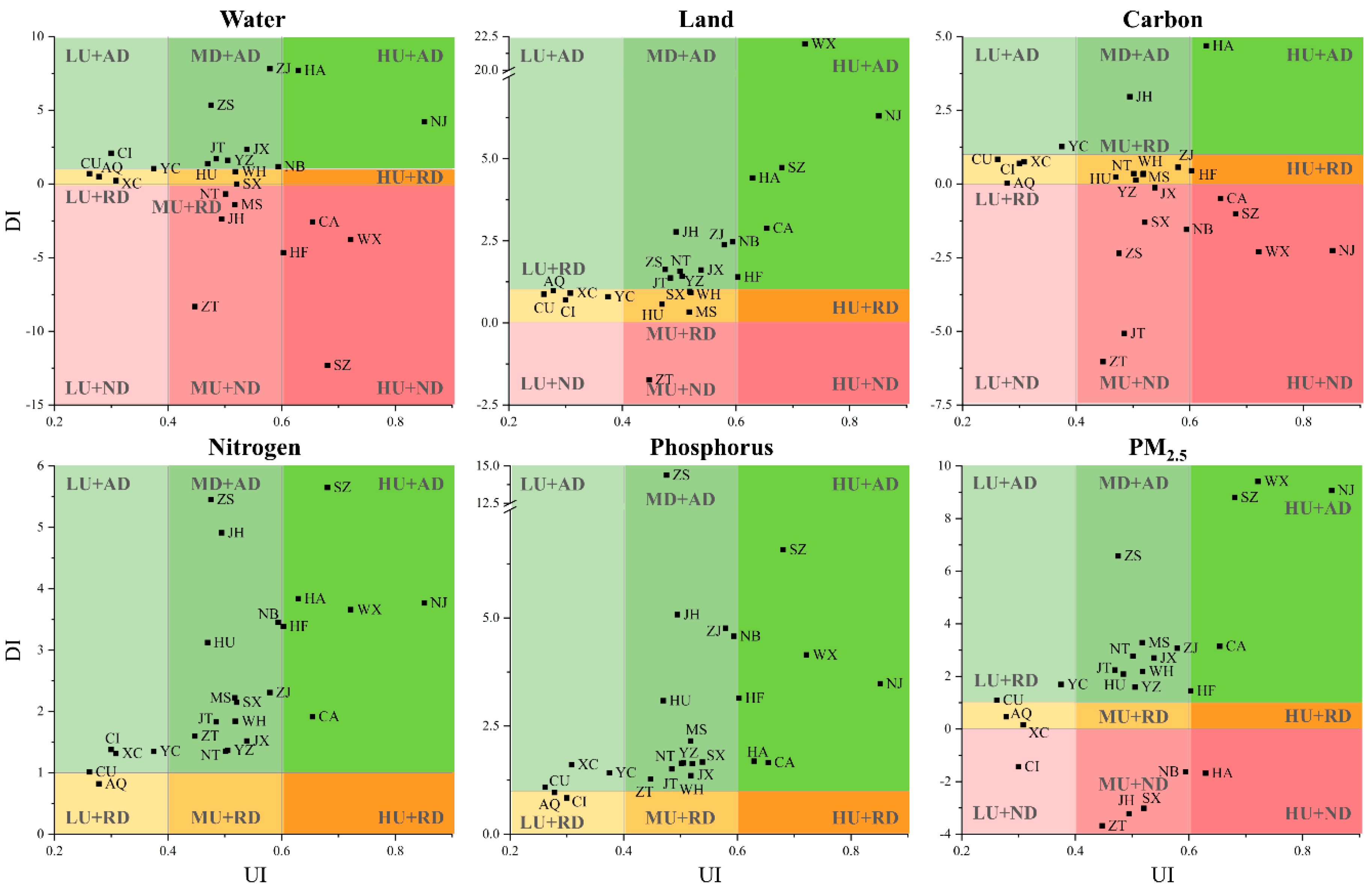
Figure 11 shows the relation between various DI and UI in 2014–2017. All five cities with low urbanization were decoupled between water ESGRs and UI, while non-decoupling occurred in some cities with higher UI, such as Suzhou and Jinhua. In terms of land DI, all low-UI cities reached relative decoupling, and all high-UI cities achieved absolute decoupling, including Nanjing, Suzhou, Wuxi, Changzhou, Hangzhou and Hefei. Low-UI cities were also found to be decoupled of carbon ESGRs, while many medium-UI and high-UI cities experienced non-decoupling. Conversely, high-UI cities had the highest average DI of both nitrogen and phosphorus ESGRs, followed by medium-UI cities and then low-UI cities. Moreover, the majority of cities in each level of urbanization reached decoupling of PM2.5 ESGRs. In conclusion, low-UI cities were almost decoupled with six categories of ESGRs, while medium-UI and high-UI cities mainly achieved absolute decoupling with nitrogen and phosphorus ESGRs, and presented various characteristics across other five categories.
4. Discussion
4.1. Revisiting Decoupling Analysis from a Sustainability Perspective
Most of the decoupling researches only concern whether environmental emissions or resource consumption experience asynchronous changes with socioeconomic development, leaving environmental sustainability a neglected field of analysis. However, decoupling analysis alone may be misleading for evaluating a city’s environmental performance. In the case of land footprint, 23 out of the 26 cities reached absolute or relative decoupling with urbanization. Nevertheless, after integrating ESA into decoupling analysis, we found only three out of the 23 cities operating within the land boundaries. Therefore, the remaining 20 cities faced the challenge of reducing unsustainable land use, and thus should be treated with different strategies. In that sense, decoupling does not necessarily mean a satisfactory environmental performance. This is why we attempted to improve traditional decoupling analysis by connecting with the footprint-boundary ESA framework. Besides, we selected six categories of environmental issues to conduct a footprint family, to assess the environmental pressure associated with urbanization in a more sound way. In doing so, the integrated analysis will help us better understand the role of decoupling in fulfilling SDGs, but also provide decision makers with more tangible and differentiated policy advices for regions and cities that differ from each other.
4.2. Limitations and Potential Solutions
However, this paper still has some limitations that should be overcome in future studies. First, due to the restriction on data acquisition, only an 11-year time horizon was investigated. Therefore, it makes sense to collect more data through multiple accesses and look deeper into the historical trends in the environmental and socioeconomic aspects of urban development. Second, the method used in this paper was limited in capturing spatial characteristics. Because of this, the adoption of spatial econometric models is expected. Third, although this paper explored the possible relation between decoupling and urbanization, and other driving factors influencing the decoupling were not discussed. To yield more concrete policy recommendations, there is a need for identifying more socioeconomic driving factors.
Finally, downscaled planetary carbon, nitrogen and phosphorus boundaries employed in this paper followed the principle of sharing global environmental responsibility and could provide a reference benchmark to ESA at the city level. Nevertheless, downscaling planetary boundaries to sub-global levels is a complicated issue that has relation to biophysical, socioeconomic and ethical considerations, inevitably involving uncertainties and subjectivity [71]. For instance, per capita allocation pertaining to egalitarian neglects spatial heterogeneity of biophysical processes, and therefore is a source of controversy in determining sub-global environmental boundaries. Meanwhile, measuring nitrogen and phosphorus boundaries at a city level with a bottom-up approach is a very costly and tough engineering task, and thus goes beyond the scope of this paper. Similar critiques also apply to the downscaling of the planetary water and land boundaries. As such, further improvements need to focus on how to strengthen the policy relevance of the planetary boundaries which should be applied at the ecosystem level or below. In addition, trade-off analysis between various environmental issues assessed in our study would be needed as well.
4.3. Policy Implications
Cities account for the overwhelming majority of resources consumption and environmental emissions, thus posing a substantial obstacle to building sustainable cities as declared in the SDGs. Policy advices on the optimal pathways towards sustainable development for six patterns of cities in the YRD at the city level are drawn as follows:
For the cities that have fallen into “EU + ND”, great emphasis should be placed on environmental protection. We suggest that these cities should find ways to control the growth of environmental sustainability gaps and take immediate actions to achieve decoupling from urbanization. For example, all the YRD cities are found to be unsustainable in terms of climate change between 2007 and 2017. Therefore, it is necessary to improve energy efficiency, introduce more low-carbon technologies, and develop renewable energy [72], especially for 10 “EU + ND” cities (e.g., Suzhou and Ningbo).
We believe that the “EU + RD” cities slow down the increase in environmental sustainability gaps, to finally achieve absolute decoupling. For instance, nine cities with environmental unsustainability of land use are still relatively decoupled with urbanization in 2014–2017, such as Shaoxing and Maanshan. These cities should give priority to improving land-use planning under the ecological redline policy [73], and to raising land-use efficiency [74].
The “EU + AD” cities showed a positive sign towards environmental sustainability. We advise that these cities should try their best to maintain the absolute decoupling trend, and to shift from environmental unsustainability to sustainability as soon as possible. In the case of PM2.5 emissions, 15 absolutely decoupled cities should continue to reduce vehicle emissions and promote clean energy [75], in order to lower PM2.5 concentrations.
The remaining cities are all in a state of environmental sustainability, including the “ES + AD”, “ES + RD” and “ES + ND” ones. Although these cities have not yet transgressed the permissible boundaries, some of their environmental sustainability gaps increased as a result of urbanization. For example, a growth in environmental sustainability gaps of water use was observed in five out of nine sustainable cities. Therefore, we consider decoupling of environmental sustainability gaps from urbanization remains as a prioritized goal, particularly for those classified into “ES + ND” and “ES + RD”.
5. Conclusions
This paper evaluated the environmental sustainability of water use, land use, carbon emissions, nitrogen emissions, phosphorus emissions and PM2.5 emissions in the 26 cities among the YRD urban agglomerations, and explored the decoupling of environmental sustainability gaps from urbanization. The results indicated that nine cities reached the environmental sustainability of water use in 2017. Environmental sustainability of land use showed notable spatial heterogeneity, on which Anhui and Jiangsu performed better than Shanghai and Zhejiang. Carbon emissions in all the cities investigated operated in a state of environmental unsustainability over the entire study period 2007–2017, due to the fact that the planetary boundaries for climate change have already been considerably transgressed. The environmental sustainability of nitrogen and phosphorus emissions exhibited similar spatiotemporal characteristics, for which seven and six cities were kept within the corresponding boundaries, respectively. The environmental sustainability gaps of PM2.5 emissions experienced an increasing trend from coastal cities to inland cities. During the study period, a continuous growth in urbanization was witnessed in the YRD. Decoupling analysis showed that there were 15, 23, 14, 24, 24 and 18 cities reached the decoupling of six categories of environmental sustainability gaps from urbanization in 2014–2017, respectively. Noticeably, most of the cities achieved absolute decoupling with environmental sustainability gaps of nitrogen and phosphorus emissions during the entire period. Furthermore, this paper revisited decoupling analysis by incorporating ESA, and then categorized all the cities into six patterns based on the integrated evaluation. Policy recommendations for seeking optimal pathways towards sustainable development were proposed for each pattern. Overall, the integration of ESA and decoupling analysis enables a more sound evaluation of environmental performance in the context of rapid urbanization, thus being able to assist decision makers in formulating more feasible and differentiated policies in the pursuit of SDGs.
Author Contributions
Y.H. and J.Z. contributed equally to this work. Conceptualization, J.W.; methodology, Y.H. and J.Z.; formal analysis, Y.H. and J.Z.; data curation, Y.H. and J.Z.; writing—original draft preparation, Y.H. and J.Z.; writing—review and editing, J.W.; visualization, Y.H.; project administration, J.W.; funding acquisition, J.W. All authors have read and agreed to the published version of the manuscript.
Funding
This research was funded by “The Major Project of National Social Science Fund of China, grant number 20ZDA088”.
Conflicts of Interest
The authors declare no conflict of interest.
References
- National Bureau of Statistics of the People’s Republic of China. Available online: http://data.stats.gov.cn/easyquery.htm?cn=C01&zb=A0305&sj=2019 (accessed on 13 August 2020).
- Bai, X.; McPhearson, T.; Cleugh, H.; Nagendra, H.; Tong, X.; Zhu, T.; Zhu, Y. Linking Urbanization and the Environment: Conceptual and Empirical Advances. Annu. Rev. Environ. Resour. 2017, 42, 215–240. [Google Scholar] [CrossRef] [Green Version]
- Yu, S.; Yu, G.B.; Liu, Y.; Li, G.; Feng, S.; Wu, S.C.; Wong, M.H. Urbanization impairs surface water quality: Eutrophication and metal stress in the grand canal of China. River Res. Appl. 2011, 28, 1135–1148. [Google Scholar] [CrossRef]
- He, C.; Zhou, L.; Ma, W.; Wang, Y. Spatial Assessment of Urban Climate Change Vulnerability during Different Urbanization Phases. Sustainability 2019, 11, 2406. [Google Scholar] [CrossRef] [Green Version]
- Silver, B.; Reddington, C.L.; Arnold, S.R.; Spracklen, D.V. Substantial changes in air pollution across China during 2015–2017. Environ. Res. Lett. 2018, 13, 114012. [Google Scholar] [CrossRef]
- Li, W.; Hai, X.; Han, L.; Mao, J.; Tian, M. Does urbanization intensify regional water scarcity? Evidence and implications from a megaregion of China. J. Clean. Prod. 2020, 244, 118592. [Google Scholar] [CrossRef]
- Fang, K.; Wang, T.; He, J.; Wang, T.; Xie, X.; Tang, Y.; Shen, Y.; Xu, A. The distribution and drivers of PM2.5 in a rapidly urbanizing region: The Belt and Road Initiative in focus. Sci. Total Environ. 2020, 716, 137010. [Google Scholar] [CrossRef]
- Sun, Y.; Zhang, X.; Ren, G.; Zwiers, F.W.; Hu, T. Contribution of urbanization to warming in China. Nat. Clim. Chang. 2016, 6, 706–709. [Google Scholar] [CrossRef]
- Song, Y.; Zhang, M.; Zhou, M. Study on the decoupling relationship between CO2 emissions and economic development based on two-dimensional decoupling theory: A case between China and the United States. Ecol. Indic. 2019, 102, 230–236. [Google Scholar] [CrossRef]
- Sarkodie, S.A.; Strezov, V. A review on Environmental Kuznets Curve hypothesis using bibliometric and meta-analysis. Sci. Total Environ. 2019, 649, 128–145. [Google Scholar] [CrossRef]
- Marques, A.C.; Fuinhas, J.A.; Leal, P. The impact of economic growth on CO2 emissions in Australia: The environmental Kuznets curve and the decoupling index. Environ. Sci. Pollut. Res. 2018, 25, 27283–27296. [Google Scholar] [CrossRef]
- Hao, Y.; Huang, Z.; Wu, H. Do Carbon Emissions and Economic Growth Decouple in China? An Empirical Analysis Based on Provincial Panel Data. Energies 2019, 12, 2411. [Google Scholar] [CrossRef] [Green Version]
- Lin, B.; Omoju, O.E.; Nwakeze, N.M.; Okonkwo, J.U.; Megbowon, E.T. Is the environmental Kuznets curve hypothesis a sound basis for environmental policy in Africa? J. Clean. Prod. 2016, 133, 712–724. [Google Scholar] [CrossRef]
- Jaligot, R.; Chenal, J. Decoupling municipal solid waste generation and economic growth in the canton of Vaud, Switzerland. Resour. Conserv. Recycl. 2018, 130, 260–266. [Google Scholar] [CrossRef]
- Fischer-Kowalski, M.; von Weizsacker, E.U.; Ren, Y.; Moriguchi, Y.; Crane, W.; Krausmann, F.; Eisenmenger, N.; Giljum, S.; Hennicke, P.; Kemp, R.; et al. Decoupling Natural Resource Use and Environmental Impacts from Economic Growth; International Resource Panel, Ed.; United Nations Environment Programme: Nairobi, Kenya, 2011; pp. 1–54. [Google Scholar]
- Schandl, H.; Hatfield-Dodds, S.; Wiedmann, T.; Geschke, A.; Cai, Y.; West, J.; Newth, D.; Baynes, T.; Lenzen, M.; Owen, A. Decoupling global environmental pressure and economic growth: Scenarios for energy use, materials use and carbon emissions. J. Clean. Prod. 2016, 132, 45–56. [Google Scholar] [CrossRef]
- Pao, H.-T.; Chen, C.-C. Decoupling strategies: CO2 emissions, energy resources, and economic growth in the Group of Twenty. J. Clean. Prod. 2019, 206, 907–919. [Google Scholar] [CrossRef]
- Grand, M.C. Carbon emission targets and decoupling indicators. Ecol. Indic. 2016, 67, 649–656. [Google Scholar] [CrossRef]
- Ruffing, K. Indicators to measure decoupling of environmental pressure from economic growth. In Sustainability Indicators: A Scientific Assessment; Hák, T., Moldan, B., Dahl, A.L., Eds.; Island Press: Washington, DC, USA, 2007; pp. 211–222. [Google Scholar]
- Tapio, P. Towards a theory of decoupling: Degrees of decoupling in the EU and the case of road traffic in Finland between 1970 and 2001. Transp. Policy 2005, 12, 137–151. [Google Scholar] [CrossRef] [Green Version]
- Cohen, G.; Jalles, J.T.; Loungani, P.; Marto, R. The long-run decoupling of emissions and output: Evidence from the largest emitters. Energy Policy 2018, 118, 58–68. [Google Scholar] [CrossRef]
- Shuai, C.; Chen, X.; Wu, Y.; Zhang, Y.; Tan, Y. A three-step strategy for decoupling economic growth from carbon emission: Empirical evidences from 133 countries. Sci. Total Environ. 2018, 646, 524–543. [Google Scholar] [CrossRef]
- Moreau, V.; Vuille, F. Decoupling energy use and economic growth: Counter evidence from structural effects and embodied energy in trade. Appl. Energy 2018, 215, 54–62. [Google Scholar] [CrossRef]
- Wu, Y.; Zhu, Q.; Zhu, B. Comparisons of decoupling trends of global economic growth and energy consumption between developed and developing countries. Energy Policy 2018, 116, 30–38. [Google Scholar] [CrossRef]
- Wang, Q.; Zhao, M.; Li, R.; Su, M. Decomposition and decoupling analysis of carbon emissions from economic growth: A comparative study of China and the United States. J. Clean. Prod. 2018, 197, 178–184. [Google Scholar] [CrossRef]
- Zhang, X.; Geng, Y.; Shao, S.; Song, X.; Fan, M.; Yang, L.; Song, J. Decoupling PM2.5 emissions and economic growth in China over 1998–2016: A regional investment perspective. Sci. Total Environ. 2020, 714, 136841. [Google Scholar] [CrossRef]
- Wang, Q.; Wang, X. Moving to economic growth without water demand growth—A decomposition analysis of decoupling from economic growth and water use in 31 provinces of China. Sci. Total Environ. 2020, 726, 138362. [Google Scholar] [CrossRef]
- Szigeti, C.; Toth, G.; Szabo, D.R. Decoupling—Shifts in ecological footprint intensity of nations in the last decade. Ecol. Indic. 2017, 72, 111–117. [Google Scholar] [CrossRef]
- Fan, W.; Meng, M.; Lu, J.; Dong, X.; Fan, W.; Wang, X.; Zhang, Q. Decoupling Elasticity and Driving Factors of Energy Consumption and Economic Development in the Qinghai-Tibet Plateau. Sustainability 2020, 12, 1326. [Google Scholar] [CrossRef] [Green Version]
- Yu, Y.; Chen, D.; Zhu, B.; Hu, S. Eco-efficiency trends in China, 1978–2010: Decoupling environmental pressure from economic growth. Ecol. Indic. 2013, 24, 177–184. [Google Scholar] [CrossRef]
- Hatfield-Dodds, S.; Schandl, H.; Adams, P.D.; Baynes, T.; Brinsmead, T.S.; Bryan, B.A.; Chiew, F.H.S.; Graham, P.; Grundy, M.; Harwood, T.; et al. Australia is ‘free to choose’ economic growth and falling environmental pressures. Nature 2015, 527, 49–53. [Google Scholar] [CrossRef]
- Bithas, K.; Kalimeris, P. Unmasking decoupling: Redefining the Resource Intensity of the Economy. Sci. Total Environ. 2018, 619, 338–351. [Google Scholar] [CrossRef]
- Akizu-Gardoki, O.; Bueno, G.; Wiedmann, T.; Lopez-Guede, J.M.; Arto, I.; Hernandez, P.; Moran, D. Decoupling between human development and energy consumption within footprint accounts. J. Clean. Prod. 2018, 202, 1145–1157. [Google Scholar] [CrossRef]
- Cibulka, S.; Giljum, S. Towards a Comprehensive Framework of the Relationships between Resource Footprints, Quality of Life, and Economic Development. Sustainability 2020, 12, 4734. [Google Scholar] [CrossRef]
- Yang, Y.; Liu, Y.; Li, Y.; Li, J. Measure of urban-rural transformation in Beijing-Tianjin-Hebei region in the new millennium: Population-land-industry perspective. Land Use Policy 2018, 79, 595–608. [Google Scholar] [CrossRef]
- Liang, W.; Yang, M. Urbanization, economic growth and environmental pollution: Evidence from China. Sustain. Comput. Inform. Syst. 2019, 21, 1–9. [Google Scholar] [CrossRef]
- Bao, C.; Zou, J. Exploring the Coupling and Decoupling Relationships between Urbanization Quality and Water Resources Constraint Intensity: Spatiotemporal Analysis for Northwest China. Sustainability 2017, 9, 1960. [Google Scholar] [CrossRef] [Green Version]
- Wang, T.; Riti, J.S.; Shu, Y. Decoupling emissions of greenhouse gas, urbanization, energy and income: Analysis from the economy of China. Environ. Sci. Pollut. Res. 2018, 25, 19845–19858. [Google Scholar] [CrossRef]
- Ariken, M.; Zhang, F.; Liu, K.; Fang, C.; Kung, H.-T. Coupling coordination analysis of urbanization and eco-environment in Yanqi Basin based on multi-source remote sensing data. Ecol. Indic. 2020, 114, 106331. [Google Scholar] [CrossRef]
- Wang, Z.; Liang, L.; Sun, Z.; Wang, X. Spatiotemporal differentiation and the factors influencing urbanization and ecological environment synergistic effects within the Beijing-Tianjin-Hebei urban agglomeration. J. Environ. Manag. 2019, 243, 227–239. [Google Scholar] [CrossRef]
- Wang, J.; Wang, S.; Li, S.; Feng, K. Coupling analysis of urbanization and energy-environment efficiency: Evidence from Guangdong province. Appl. Energy 2019, 254, 113650. [Google Scholar] [CrossRef]
- Moldan, B.; Janoušková, S.; Hak, T. How to understand and measure environmental sustainability: Indicators and targets. Ecol. Indic. 2012, 17, 4–13. [Google Scholar] [CrossRef]
- Fang, K.; Heijungs, R.; De Snoo, G.R. Understanding the complementary linkages between environmental footprints and planetary boundaries in a footprint–boundary environmental sustainability assessment framework. Ecol. Econ. 2015, 114, 218–226. [Google Scholar] [CrossRef]
- Ekins, P. Environmental sustainability: From environmental valuation to the sustainability gap. Prog. Phys. Geogr. 2011, 35, 629–651. [Google Scholar] [CrossRef]
- Hoekstra, A.Y.; Wiedmann, T. Humanity’s unsustainable environmental footprint. Science 2014, 344, 1114–1117. [Google Scholar] [CrossRef]
- Galli, A.; Wiedmann, T.; Ercin, A.E.; Knoblauch, D.; Ewing, B.; Giljum, S. Integrating Ecological, Carbon and Water footprint into a “Footprint Family” of indicators: Definition and role in tracking human pressure on the planet. Ecol. Indic. 2012, 16, 100–112. [Google Scholar] [CrossRef]
- Fang, K.; Heijungs, R.; De Snoo, G.R. Theoretical exploration for the combination of the ecological, energy, carbon, and water footprints: Overview of a footprint family. Ecol. Indic. 2014, 36, 508–518. [Google Scholar] [CrossRef]
- Lin, D.; Hanscom, L.; Murthy, A.; Galli, A.; Evans, M.; Neill, E.; Mancini, M.S.; Martindill, J.; Medouar, F.-Z.; Huang, S.; et al. Ecological Footprint Accounting for Countries: Updates and Results of the National Footprint Accounts, 2012–2018. Resources 2018, 7, 58. [Google Scholar] [CrossRef] [Green Version]
- Wiedmann, T.; Minx, J. A definition of ‘carbon footprint’. Ecol. Econ. Res. Trends 2008, 1, 1–11. [Google Scholar]
- Hoekstra, A.Y.; Mekonnen, M.M. The water footprint of humanity. Proc. Natl. Acad. Sci. USA 2012, 109, 3232–3237. [Google Scholar] [CrossRef] [Green Version]
- Leach, A.M.; Galloway, J.N.; Bleeker, A.; Erisman, J.W.; Kohn, R.; Kitzes, J. A nitrogen footprint model to help consumers understand their role in nitrogen losses to the environment. Environ. Dev. 2012, 1, 40–66. [Google Scholar] [CrossRef] [Green Version]
- Li, M.; Wiedmann, T.; Hadjikakou, M. Towards meaningful consumption-based planetary boundary indicators: The phosphorus exceedance footprint. Glob. Environ. Chang. 2019, 54, 227–238. [Google Scholar] [CrossRef]
- Yang, S.; Chen, B.; Wakeel, M.; Hayat, T.; Alsaedi, A.; Ahmad, B. PM2.5 footprint of household energy consumption. Appl. Energy 2018, 227, 375–383. [Google Scholar] [CrossRef]
- Rockström, J.; Steffen, W.; Noone, K.; Persson, Å.; Chapin, F.S.; Lambin, E.F.; Lenton, T.M.; Scheffer, M.; Folke, C.; Schellnhuber, H.J.; et al. A safe operating space for humanity. Nature 2009, 461, 472–475. [Google Scholar] [CrossRef]
- Shao, S.; Chen, Y.; Li, K.; Yang, L. Market segmentation and urban CO2 emissions in China: Evidence from the Yangtze River Delta region. J. Environ. Manag. 2019, 248, 109324. [Google Scholar] [CrossRef]
- National Development and Reform Commission of the People’s Republic of China. Available online: https://www.ndrc.gov.cn/xxgk/zcfb/ghwb/201606/t20160603_962187.html (accessed on 13 August 2020).
- Fang, K.; Heijungs, R.; Duan, Z.; De Snoo, G.R. The Environmental Sustainability of Nations: Benchmarking the Carbon, Water and Land Footprints against Allocated Planetary Boundaries. Sustainanility 2015, 7, 11285–11305. [Google Scholar] [CrossRef] [Green Version]
- 2006 IPCC Guidelines for National Greenhouse Gas Inventories. Available online: https://www.ipcc.ch/report/2006-ipcc-guidelines-for-national-greenhouse-gas-inventories/ (accessed on 16 August 2020).
- Goldberg, M.H.; Van Der Linden, S.; Maibach, E.; Leiserowitz, A. Discussing global warming leads to greater acceptance of climate science. Proc. Natl. Acad. Sci. USA 2019, 116, 14804–14805. [Google Scholar] [CrossRef] [Green Version]
- Chakrabarti, S. Eutrophication—A global aquatic environmental problem: A review. Res. Rev. J. Ecol. Environ. Sci. 2018, 6, 1–6. [Google Scholar]
- Lucas, P.L.; Wilting, H.C.; Hof, A.F.; Van Vuuren, D.P. Allocating planetary boundaries to large economies: Distributional consequences of alternative perspectives on distributive fairness. Glob. Environ. Chang. 2020, 60, 102017. [Google Scholar] [CrossRef]
- Hjalsted, A.W.; Laurent, A.; Andersen, M.M.; Olsen, K.H.; Ryberg, M.; Hauschild, M. Sharing the safe operating space: Exploring ethical allocation principles to operationalize the planetary boundaries and assess absolute sustainability at individual and industrial sector levels. J. Ind. Ecol. 2020, 1–14. [Google Scholar] [CrossRef]
- Ministry of Ecology and Environment of the People’s Republic of China. Available online: http://www.mee.gov.cn/xxgk2018/xxgk/xxgk15/201808/t20180815_630438.html (accessed on 28 June 2020).
- Van Donkelaar, A.; Martin, R.V.; Brauer, M.; Hsu, N.C.; Kahn, R.A.; Levy, R.C.; Lyapustin, A.; Sayer, A.M.; Winker, D.M. Global Estimates of Fine Particulate Matter using a Combined Geophysical-Statistical Method with Information from Satellites, Models, and Monitors. Environ. Sci. Technol. 2016, 50, 3762–3772. [Google Scholar] [CrossRef]
- Liu, M.; Li, W. Calculation of equivalence factor used in ecological footprint for China and its provinces based on net primary production. J. Ecol. Rural Environ. 2010, 26, 401–406. (In Chinese) [Google Scholar]
- Xie, H.; Ye, H. The update computation for global average yield of main agricultural products in China. J. Guangzhou Univ. (Nat. Sci. Ed.) 2008, 7, 76–80. (In Chinese) [Google Scholar]
- Kahrl, F.; Li, Y.; Su, Y.; Tennigkeit, T.; Wilkes, A.; Xu, J. Greenhouse gas emissions from nitrogen fertilizer use in China. Environ. Sci. Policy 2010, 13, 688–694. [Google Scholar] [CrossRef]
- Wu, H.; Wang, S.; Gao, L.; Zhang, L.; Yuan, Z.; Fan, T.; Wei, K.; Huang, L. Nutrient-derived environmental impacts in Chinese agriculture during 1978–2015. J. Environ. Manag. 2018, 217, 762–774. [Google Scholar] [CrossRef]
- O’Neill, D.W.; Fanning, A.L.; Lamb, W.F.; Steinberger, J.K. A good life for all within planetary boundaries. Nat. Sustain. 2018, 1, 88–95. [Google Scholar] [CrossRef] [Green Version]
- Liu, M.; Li, W.; Xie, G. Estimation of China ecological footprint production coefficient based on net primary productivity. Chin. J. Ecol. 2010, 29, 592–597. (In Chinese) [Google Scholar]
- Hachaichi, M.; Baouni, T. Downscaling the planetary boundaries (Pbs) framework to city scale-level: De-risking MENA region’s environment future. Environ. Sustain. Indic. 2020, 5, 100023. [Google Scholar] [CrossRef]
- Hertwich, E.; Gibon, T.; Bouman, E.A.; Arvesen, A.; Suh, S.; Heath, G.A.; Bergesen, J.D.; Ramírez, A.; Vega, M.I.; Shi, L. Integrated life-cycle assessment of electricity-supply scenarios confirms global environmental benefit of low-carbon technologies. Proc. Natl. Acad. Sci. USA 2014, 112, 6277–6282. [Google Scholar] [CrossRef] [Green Version]
- Bai, Y.; Wong, C.P.; Jiang, B.; Hughes, A.C.; Wang, M.; Wang, Q. Developing China’s Ecological Redline Policy using ecosystem services assessments for land use planning. Nat. Commun. 2018, 9, 3034. [Google Scholar] [CrossRef] [Green Version]
- Yu, J.; Zhou, K.; Yang, S. Land use efficiency and influencing factors of urban agglomerations in China. Land Use Policy 2019, 88, 104143. [Google Scholar] [CrossRef]
- Li, Y.; Chang, M.; Ding, S.; Wang, S.; Ni, D.; Hu, H. Monitoring and source apportionment of trace elements in PM 2.5: Implications for local air quality management. J. Environ. Manag. 2017, 196, 16–25. [Google Scholar] [CrossRef]
Figure 1.
Classification of decoupling degrees.
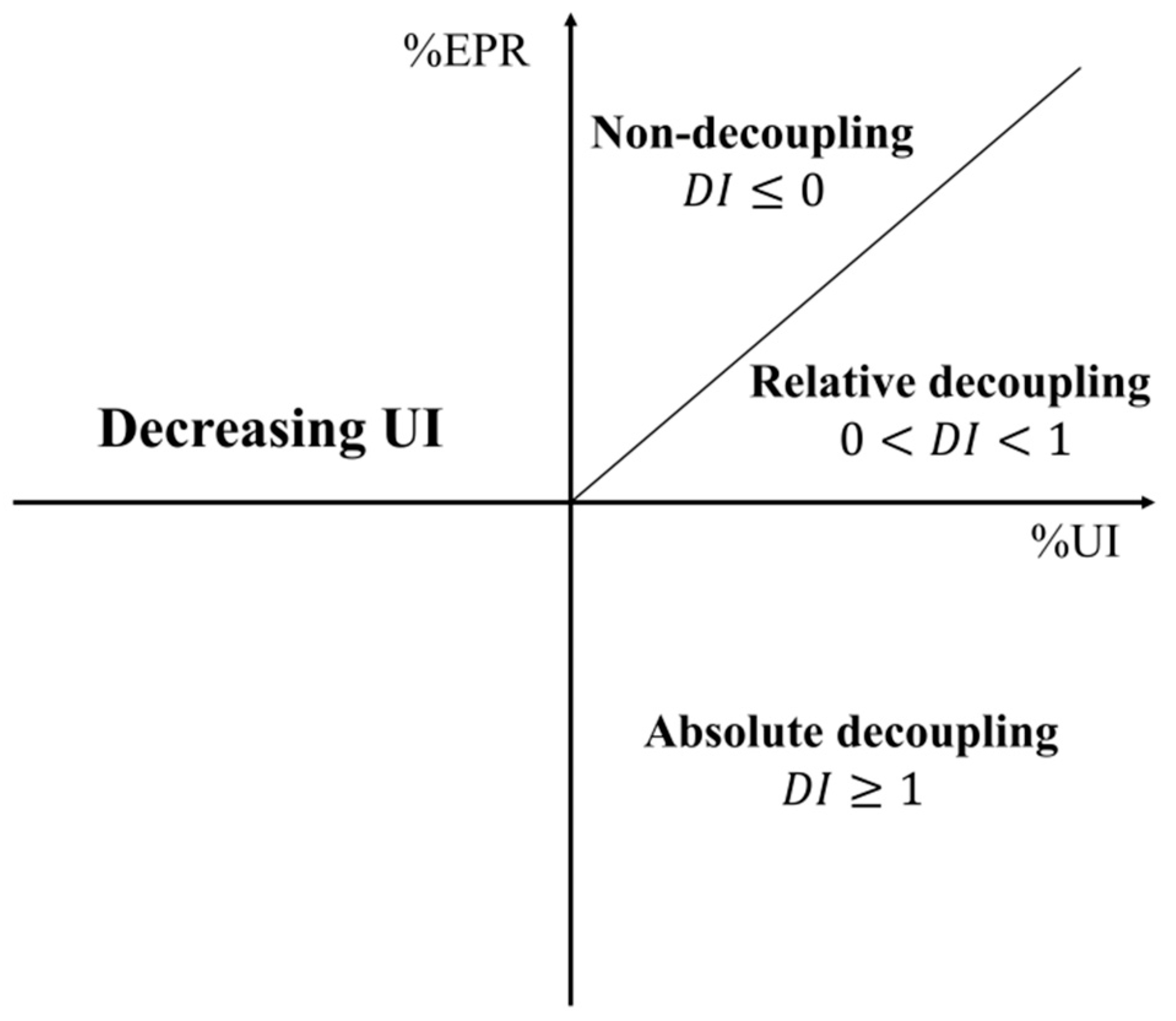
Figure 2.
Spatial distribution of water, land, carbon, nitrogen, phosphorus and PM2.5 environmental sustainability gap ratios (ESGRs) in 2017. Cities in a state of environmental sustainability ( or ) are marked in blue, while cities in a state of environmental unsustainability ( or ) are marked in red.
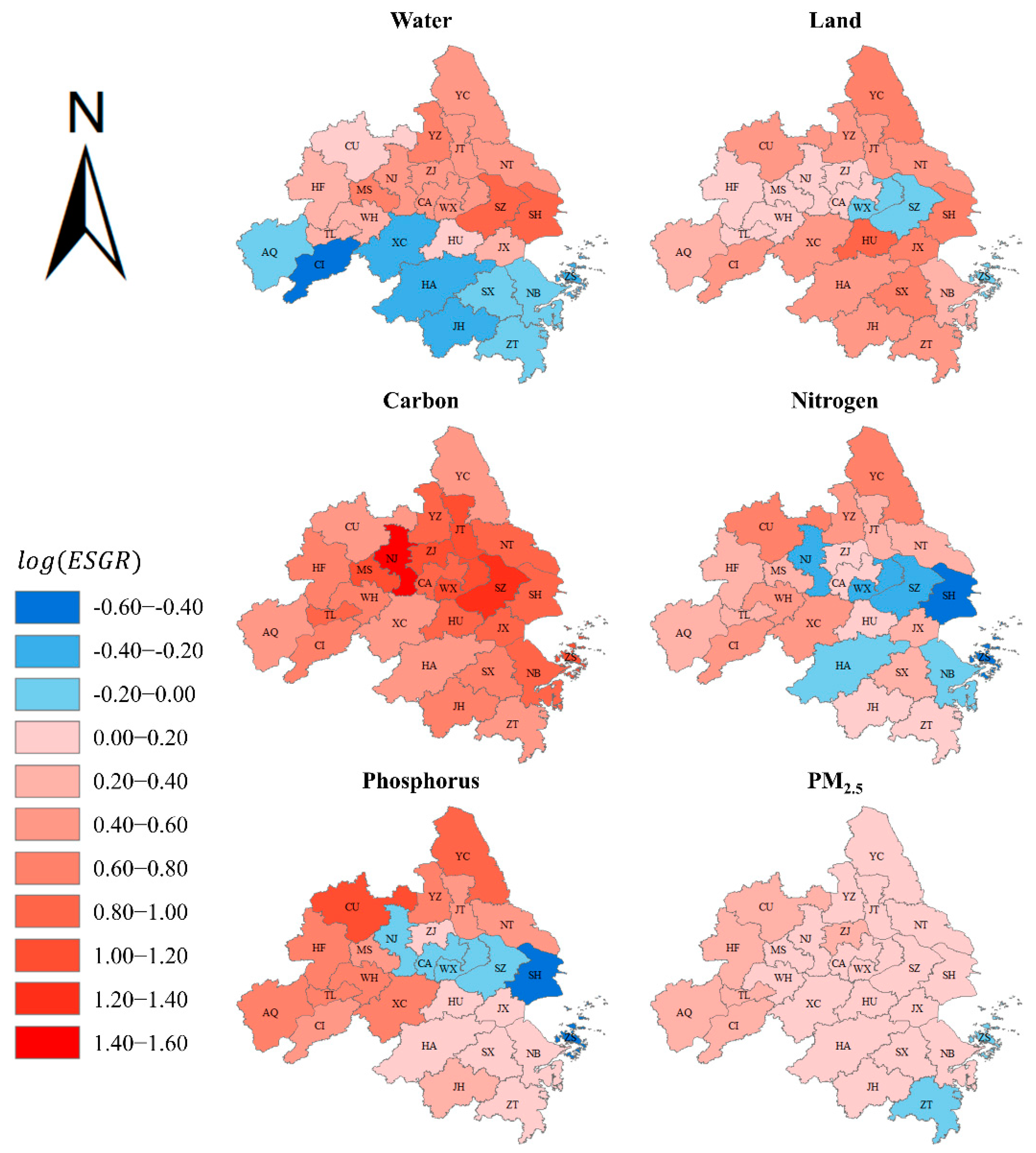
Figure 3.
Time-series performance on urbanization index in 2007, 2011, 2014 and 2017.
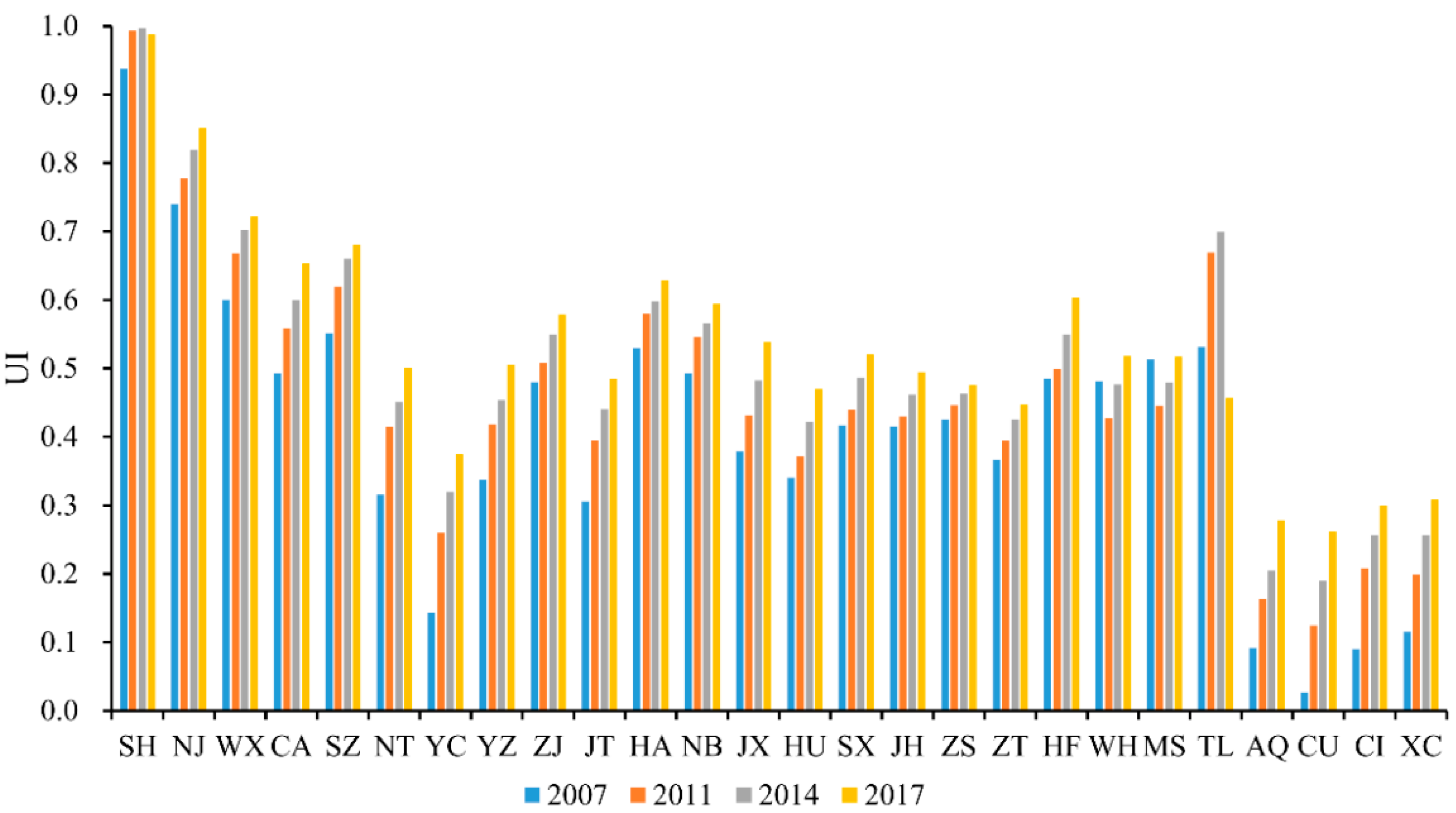
Figure 4.
Water decoupling index versus ESGRs during three periods. All the cities were classified into six patterns based on the decoupling analysis and environmental sustainability assessment (see Section 3.3 for details). Absolute decoupling (abbreviated as “AD”) zones are colored in green, relative decoupling (abbreviated as “RD”) zones are colored in yellow, and non-decoupling (abbreviated as “ND”) zones are colored in red. Environmental sustainability (abbreviated as “ES”) zones are colored darker than the corresponding environmental unsustainability (abbreviated as “EU”) zones. The same below.
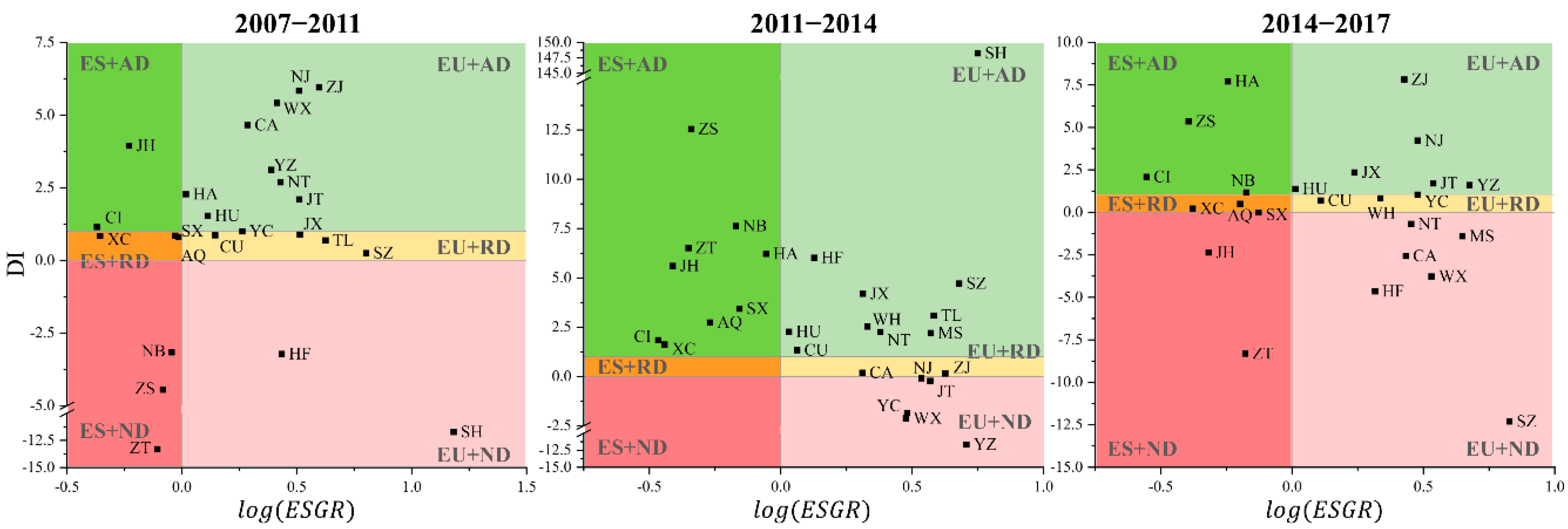
Figure 5.
Land DI versus ESGRs during three periods.

Figure 6.
Carbon DI versus ESGRs during three periods.
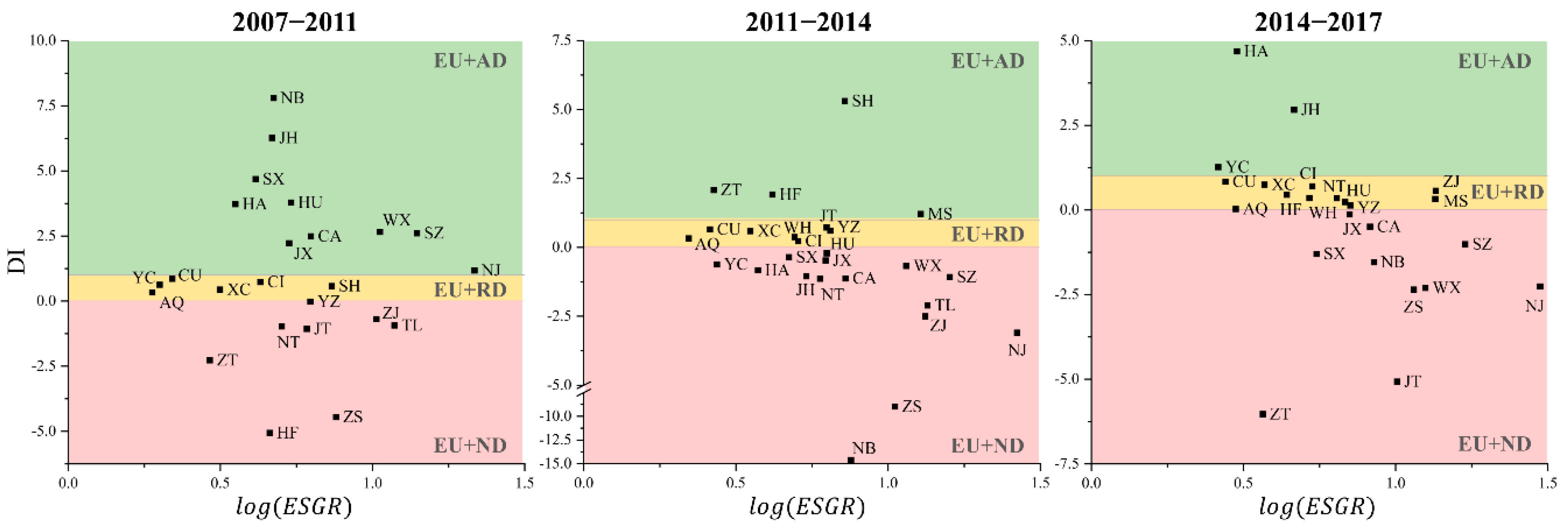
Figure 7.
Nitrogen DI versus ESGRs during three periods.

Figure 8.
Phosphorus DI versus ESGRs during three periods.
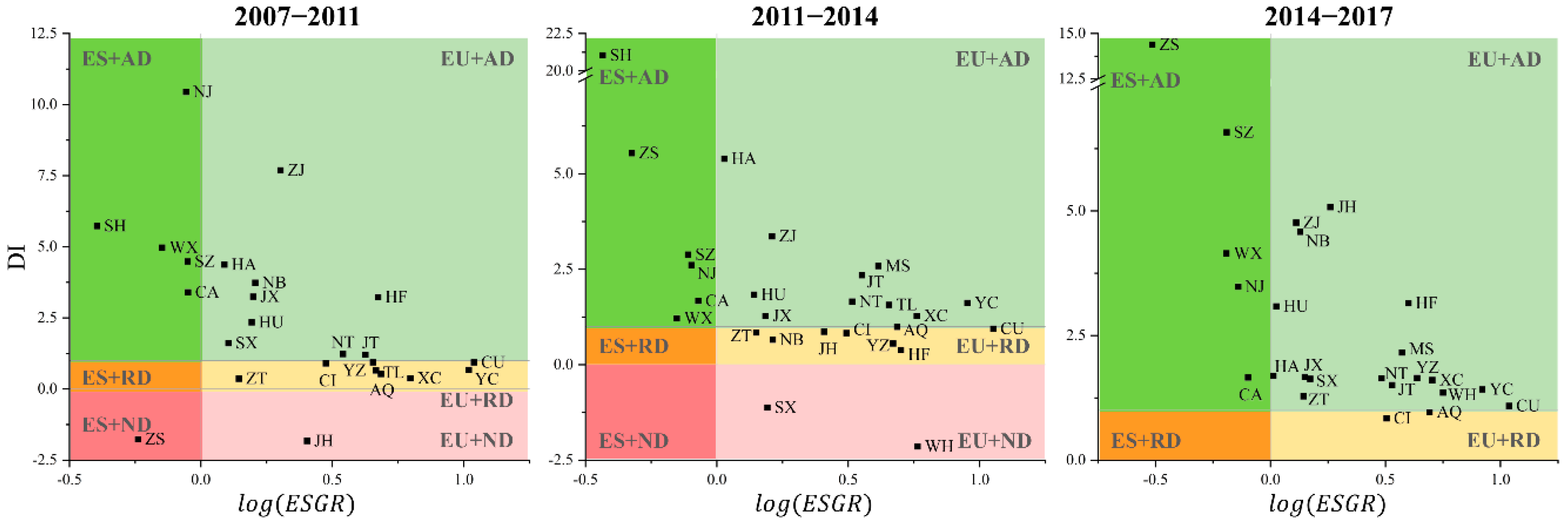
Figure 9.
PM2.5 DI versus ESGRs during three periods.

Figure 10.
The percentage of decoupling degrees for water, land, carbon, nitrogen, phosphorus and PM2.5 ESGRs in 2014–2017.
Figure 10.
The percentage of decoupling degrees for water, land, carbon, nitrogen, phosphorus and PM2.5 ESGRs in 2014–2017.

Figure 11.
Water, land, carbon, nitrogen, phosphorus and PM2.5 DI versus UI in 2014–2017. All the cities were classified into nine patterns based on the decoupling degrees and urbanization levels. High urbanization (abbreviated as “HU”) zones are colored in darkest, the corresponding medium urbanization (abbreviated as “MU”) zones are colored in lighter, and the corresponding low urbanization (abbreviated as “LU”) zones are colored in lightest.

Table 1.
List of city codes in the Yangtze River Delta.
| City | Abbreviation | City | Abbreviation |
|---|---|---|---|
| Anqing | AQ | Shanghai | SH |
| Changzhou | CA | Shaoxing | SX |
| Chizhou | CI | Suzhou | SZ |
| Chuzhou | CU | Taizhou (in Jiangsu) | JT |
| Hangzhou | HA | Taizhou (in Zhejiang) | ZT |
| Hefei | HF | Tongling | TL |
| Huzhou | HU | Wuhu | WH |
| Jiaxing | JX | Wuxi | WX |
| Jinhua | JH | Xuancheng | XC |
| Maanshan | MS | Yancheng | YC |
| Nanjing | NJ | Yangzhou | YZ |
| Nantong | NT | Zhenjiang | ZJ |
| Ningbo | NB | Zhoushan | ZS |
Table 2.
Variable and data sources.
| Variables | Data Sources |
|---|---|
| Annual PM2.5 concentration | NASA Socioeconomic Data and Applications Center [64], and the 26 cities’ ecological environment quality bulletins |
| Areas for cropland, grassland, forestland, water area and built-up area | The statistical yearbooks of Shanghai, Jiangsu Province, Zhejiang Province, Anhui Province and the 25 cities (2008–2018) |
| Energy consumption | |
| Nitrogenous, phosphatic and compound fertilizers | |
| Regional and urban population | |
| Regional land area and urban built-up area | |
| Regional GDP and value added of secondary and tertiary industries | |
| Yields for agricultural, animal, forest and aquatic products | |
| Equivalence factors for cropland, grassland, forestland, water area and built-up area | Liu and Li [65] |
| Global average yields for agricultural, animal, forest and aquatic products | Xie and Ye [66] |
| Nitrogen and phosphorus content of compound fertilizer | Kahrl et al. [67] and Wu et al. [68] |
| Per capita carbon, nitrogen and phosphorus planetary boundaries | O’Neill et al. [69] |
| Renewable water resources | The 26 cities’ water resources bulletins (2007–2017) |
| Water consumption | Shanghai, Jiangsu, Zhejiang and Anhui water resources bulletins (2007–2017) |
| Yield factors for cropland, grassland, forestland, water area and built-up area | Liu et al. [70] |
© 2020 by the authors. Licensee MDPI, Basel, Switzerland. This article is an open access article distributed under the terms and conditions of the Creative Commons Attribution (CC BY) license (http://creativecommons.org/licenses/by/4.0/).
Share and Cite
MDPI and ACS Style
Huang, Y.; Zhang, J.; Wu, J. Integrating Sustainability Assessment into Decoupling Analysis: A Focus on the Yangtze River Delta Urban Agglomerations. Sustainability 2020, 12, 7872. https://doi.org/10.3390/su12197872
AMA Style
Huang Y, Zhang J, Wu J. Integrating Sustainability Assessment into Decoupling Analysis: A Focus on the Yangtze River Delta Urban Agglomerations. Sustainability. 2020; 12(19):7872. https://doi.org/10.3390/su12197872
Chicago/Turabian StyleHuang, Yijia, Jiaqi Zhang, and Jinqun Wu. 2020. "Integrating Sustainability Assessment into Decoupling Analysis: A Focus on the Yangtze River Delta Urban Agglomerations" Sustainability 12, no. 19: 7872. https://doi.org/10.3390/su12197872
Note that from the first issue of 2016, this journal uses article numbers instead of page numbers. See further details here.