Article

Possibilities of House Valuation Automation in the Czech Republic

Department of Urban Engineering, Faculty of Civil Engineering, VSB-Technical University of Ostrava, 708 00 Ostrava-Poruba, Czech Republic
*
Author to whom correspondence should be addressed.
Sustainability 2020, 12(18), 7774; https://doi.org/10.3390/su12187774
Submission received: 18 August 2020 / Revised: 16 September 2020 / Accepted: 17 September 2020 / Published: 20 September 2020
(This article belongs to the Section Economic and Business Aspects of Sustainability)

Abstract

:
Valuation of single-family detached houses is necessary when determining the amounts of some taxes. The current systems of the Czech Republic are outdated in this respect, and they are based on procedures used in the 1980s. The values found do not correspond to current market conditions very often. This article attempts to verify the applicability of a methodology where the value of a detached house is decomposed into the value of the land and the value of the object as such when considering wear. For verification, 122 sales of detached houses in Ostrava and its surroundings were analyzed, and the results show that the values determined by the verified methodology do not differ by more than 10% from the actual sales prices in most cases. The methodology is very simple and practically applicable for users without deep knowledge of construction or valuation principles. It can be applied, for example, when calculating the bases of certain taxes or as an indicative guide for the pricing of real estate for sellers, buyers, real estate agents, etc.

1. Introduction

Two practices are currently used to appraise real estate in the Czech Republic. The first of these is market valuation, or determination of the value for which the asset is feasibly sellable on the open market. This type of appraisal is a better reflection of the actual situation on the real estate market; however, its particular disadvantage is the fact that the procedures for performing such a valuation are only recommended, and the result is therefore influenced by the valuer’s subjective opinions and feelings. Appraisal is therefore a science and an art to a specific degree [1]. The second method is calculation of the so-called administrative (or official) value, which is determined by a procedure in accordance with the relevant jurisdiction. The procedure for calculation is firmly set, and there is little opportunity for subjective opinion. However, the administrative value quite often differs from the market value by several tens of percent.
From the economic perspective, real estate is a very specific asset, and the market for these assets is very specific and different from markets for classic commercial products (this is due, for example, to external factors influencing the price, a very limited range being offered at a specific time, etc.). This means that the actual real estate valuation process is also specific. We can find many historic opinions on how appraisal should be carried out, but three approaches are currently used most often. These are the cost approach, income approach, and market approach [2]. In relation to this, Ozdilek [3] states that these essentially concern approaches based on a view of the past (comparison with other previous sales), a view of the present (determination of the current costs of construction), and a view of the future (capitalization of future estimated income). When determining market values, the comparable transaction method is used most often [4]. However, in some cases, when using this method, one can encounter the problem of a lack of data due to the low frequency of sale of similar objects [1].
The main purpose of automated systems is to objectify the entire valuation process as much as possible and, thus, to ensure the greatest possible transparency in the real estate market. The first simple automated systems were developed in the 1980s [5].
At present, a number of automated systems are presented in the professional literature [6,7,8]. In most cases, however, these are systems for valuing apartments [9,10]. The authors emphasize that the demand for and greater expansion of automated valuation methods will lead to greater transparency in the real estate market [11]. Hedonic models are often used. These endeavor to determine the parameters that influence the prices of assets and subsequently allocate weights to these parameters, or possibly to examine the influence of one specific element on the price [12,13]. Many models use single-stage and multi-stage regression by using the ordinary least squares method [14,15]. Recently, autoregressive models have also been developed [16], as well as models using advanced techniques, such as geographic information systems [17]. Other models use a set of known parameters and characteristics of assets as well as their associated marginal prices [18]. Very advanced models use evolutionary polynomial regression to maximize data accuracy [19].
The systems are based on available statistical data about realized real estate transactions, and they try to find relationships and connections in these sets, which are then generally interpretable—they are based on comparable transaction methods. Of course, a wider available database means more objective results [18]. The systems work with multiple regressions and they create prediction functions. Everything is based on computer databases and a set of algorithms that evaluate transactions [17].
However, the authors agree that all the factors that influence the value of an asset cannot be determined, but all models have one thing in common—that they agree that location is absolutely crucial in relation to the value of the asset. Thus, it is possible to find studies that examine the impact of positive externalities on property prices, such as places that have nice views [20], are near to public service facilities [21], are in the neighborhood of public transport [22,23], or are close to public greenery [24,25]. On the other hand, negative externalities that reduce property prices have been shown, such as being in the neighborhood of electrical facilities [26], sources of pollution [27,28], or jails [29].
It is logical that no two plots of land occupy the same place in space, and the location of each of them is unique and unchangeable. This means that it is impossible to state that two pieces of real estate have an identical price, despite being absolutely identical in all other parameters, because they will always at least have a different location. Some systems endeavor to take this fact into consideration, e.g., by considering the value depending on postcode [30] or local segmentations of the real estate market [31].
However, no system is (or can be) perfect because the final transaction price during the sale of real estate is always determined by agreement between a willing seller and a willing buyer. Furthermore, both parties are aware that they are able to influence the price of the transaction during this process [32], which means that the price of the real estate can never be determined absolutely precisely, meaning that some systems offer a range within which the specific price most probably falls [1].
With regard to the fact that ownership and transfer of real estate are subject to tax in all European states, prices of the real estate must be determined for these purposes. The procedures are subsequently determined by the relevant jurisdictions—Baraňska [33] gives a comparison of the methods used in some European countries, for example. Some governments use automated systems to deal with this issue [2]. The decree of the Property Appraisal Act was implemented for these purposes in the Czech Republic. The procedure determined by the decree can be quite easily automated, and there are several software tools that enable this, but valuation itself is a matter of several tables, which are incapable of reflecting all the circumstances that affect the value. The fact that the decree is regularly updated once a year is also a problem because the assets’ values develop much more dynamically. An automated system for appraising detached houses which would be capable of determining their price with sufficient accuracy on the basis of objectively verifiable data entered by the user, could therefore be used for the purpose of determining the base tax, and would certainly also be of interest to real estate agencies, valuers, public institutions, and other specialists in the real estate market.
Most of the development in European cities is residential real estate [34]. It is, therefore, logical that this type of asset is most often sold. Valuation of apartments is relatively simple and is also related to the potential for quite simple automation of valuation—apartments are not influenced by the value of land, and there is usually a fairly large sample of similar assets on the market that were previously sold. If the floor area and overall standard are known, then the price per square meter of a unit of a specific standard in a particular location can be quite accurately estimated and applied to the apartment that is to be evaluated. Only the development of an asset’s value over time must be taken into consideration [35].
However, the situation is quite different in relation to detached houses, and there are many more factors that influence the prices of the assets—apart from the size, location, and standard, the age, number of floors and their use, renovation work carried out, etc. are also influential. In this case, automation of valuation is much more complicated.
This paper is conceived as follows. Section 2 describes a methodology that can be used to develop an automated system for valuation of detached houses. Section 3 gives a calculation of the values of coefficients that are essential for calculating and implementing an automated system, and the functionality of the entire system is subsequently verified on a sample of 122 actually sold detached houses in the city of Ostrava and its surrounding area. Section 4 summarizes the conclusions and gives recommendations for further research.

2. Methods

The methodology for potential future automated valuation is based on the following concept. If costs for construction of a new detached house are assessed in various places, these costs only differ significantly in relation to the item of acquisition of the land, while costs for construction itself—when maintaining specific standards—are very similar. The question is, therefore, whether this can also be applied to older houses, or whether the market price of a detached house can be derived from the market value of the land in the location as well as from the size of the house and its wear.
Even a cursory look at real estate offers makes it evident that the prices of residential real estate differ in the same location, and are mainly influenced by demand for housing in a specific location. However, in locations where there is high demand for housing, both land and constructed houses are also logically expensive, or, more precisely, the factors that influence demand for land intended for construction of detached houses are the same as factors influencing demand for constructed homes in the specific locations.
If we know the total sales price of a specific house, it is easy to establish how large the land belonging to it is from the data publicly available from land registries. The market value of such a land plot can subsequently be determined on the basis of comparison with other transactions concerning sale of vacant, undeveloped land plots that occurred in that specific location in the past—naturally, with relevant modifications made by taking into consideration changes to prices over time [35]. This allows us to abstract just the price of the structure as such from the total sales price of the detached house, and if its total net floor area is known, the value per square meter of this area can also be established. The net floor area means the area demarcated by the interior surfaces of the plaster or other surface treatments of individual vertical structures, including non-load-bearing partitions [36].
However, it is not as easy to establish the floor area of a house as it is to establish the area of a plot of land—the Real Estate Registry of the Czech Republic does not register data about floor areas of individual structures. However, determination of this area is very important for valuation, also with regard to the fact that the floor area of cellar and attic spaces can be expected to have a much smaller influence on the total sales price than the floor area of standard living areas.
Of course, it would be possible to take just the built-up area into consideration for the aforementioned purposes; however, in the authors’ experience in valuating specific real estate, it is apparent that work with the net floor area is much simpler and more effective because the floor area inside the structure is easier to measure using modern laser distance meters and is easier to work with, for example, in cases when part of the structure has a different standard of use (e.g., part of the floor area of the ground floor is used as a garage, part of the attic is not modified and is used as a storage space, etc.).
The total built-up area of the structure serves as a specific guideline. This can usually be established from the cadastral map on which the outline of the object is marked, or, for newer buildings, if the actual built-up area forms a separate plot with its own plot number, the area is given in the Real Estate Registry. However, it is clearly logical that the built-up area is not equivalent to the floor area.
Another question is whether the price of a detached house can be determined by adding the value of the land to the value of the house as such; in other words, is it possible to apply the following formula to each detached house with a sufficient degree of accuracy?
HV = LV + OV,
where:
  • HV—value of the detached house (CZK),
  • LV—value of the land (CZK),
  • OV—value of the actual object itself (CZK).
As stated above, the value of the land can be determined separately by multiplying its area by the unit prices, which are usually found during sales of similar land plots in the surrounding area. The value of the land is, therefore, not unknown.
The aforementioned description indicates that the value of the structure as such is considered to be the sum of the value of the individual floors, with the understanding that the price of each floor is given as the product of the net floor area and the determined unit value. However, it is evident that the unit value of each floor may differ—e.g., the unit value of the cellar will certainly be lower than the unit value of the ground floor; the cellar is not a standard occupied space, as in most cases, there is insufficient daylight and the ceiling height is also lower. In order to simplify, we consider the coefficient of the potential to occupy the ground floor to be equal to 1; the coefficients for other floors are, therefore, unknown, as is the net value. If we consider the value of a detached house with two floors and a cellar, or one floor and an attic, the considered relationship can be mathematically written as follows:
OV = α1 × SUV × S1 + SUV × S2 + α3 × SUV × S3,
where:
  • OV—value of the actual object itself (CZK),
  • α1—coefficient taking into consideration the potential to use the cellar,
  • α3—coefficient taking into consideration the potential to use the first floor or attic,
  • SUV—structure unit value (CZK/square meter),
  • S1—net floor area of the cellar,
  • S2—net floor area of the ground floor,
  • S3—net floor area of the first floor or attic.
The product of the coefficients and the unit value of the structure can be expressed by one unknown, i.e.:
α1 × SUV = β1,
SUV = β2,
α3 × SUV = β3.
As stated above, the final price of the transaction during the sale of real estate is influenced to some degree by the subjective decisions of the involved parties, their ability to negotiate, etc. The data about prices are therefore heteroscedastic, and uncertainty must also be taken into account. If we enter formulas (3), (4), and (5) into formula (2) and enter uncertainty ε, we get the formula:
OV = β1 × S1 + β2 × S2 + β3 × S3 + ε.
The goal is therefore to determine the values of coefficients β1, β2, and β3 so that a generally applicable formula is created into which one simply enters the value of the net floor areas of the individual floors and determines the market value of the detached house to a sufficient degree of accuracy.
However, there are still several problems with the formula. The first is the fact that the aforementioned relationship does not take into consideration the standard of the object or its wear. Calculation of the estimated wear of the house is a standard element of a valuer’s work, which is why it is not discussed in more detail here. Bradáč [36] discusses this issue under the conditions of the Czech Republic in more detail, for example. Wear is given as a percentage, with the understanding that zero wear is equivalent to a new build; the more wear, the lower the structure’s standard.
Another individual problem is the fact that the prices of real estate develop over time [37]. With regard to the fact that samples of sales over the last three years were used in the practical application set out below, similarly to other models, changes to prices over time must be taken into consideration [38]. The Czech Statistical Office [39] monitors development of real estate prices in the Czech Republic, and the published data indicate that both the prices of building plots and the prices of detached houses have been rising since 2016. Growth is approximately linear from 2016, whereas the prices of detached houses increase by approximately 0.6% every month. If development of real estate prices differs over time, the relevant value must naturally be modified. The final form of the required formula in the current situation is as follows:
OV = (β1 × S1 + β2 × S2 + β3 × S3) × (1 − W) × (1 + MN × 0.006) + ε,
where:
  • W—wear given in decimal values,
  • MN—number of calendar months that have elapsed since sale.
With regard to the fact that neither wear nor time of sale are unknown, but can be determined before commencing calculation, this modification can be allowed.
The above is also the basis for several questions, which this paper endeavors to answer:
  • Can the ratio between the net floor area and built-up floor area of a detached house be determined?
  • Can the value of a detached house be determined as the product of the value of the land and the value of the house as such?
  • To what degree do cellars, attics, and other areas that are not intended for permanent occupation influence the value of a detached house?
  • Can the entire system be automated?
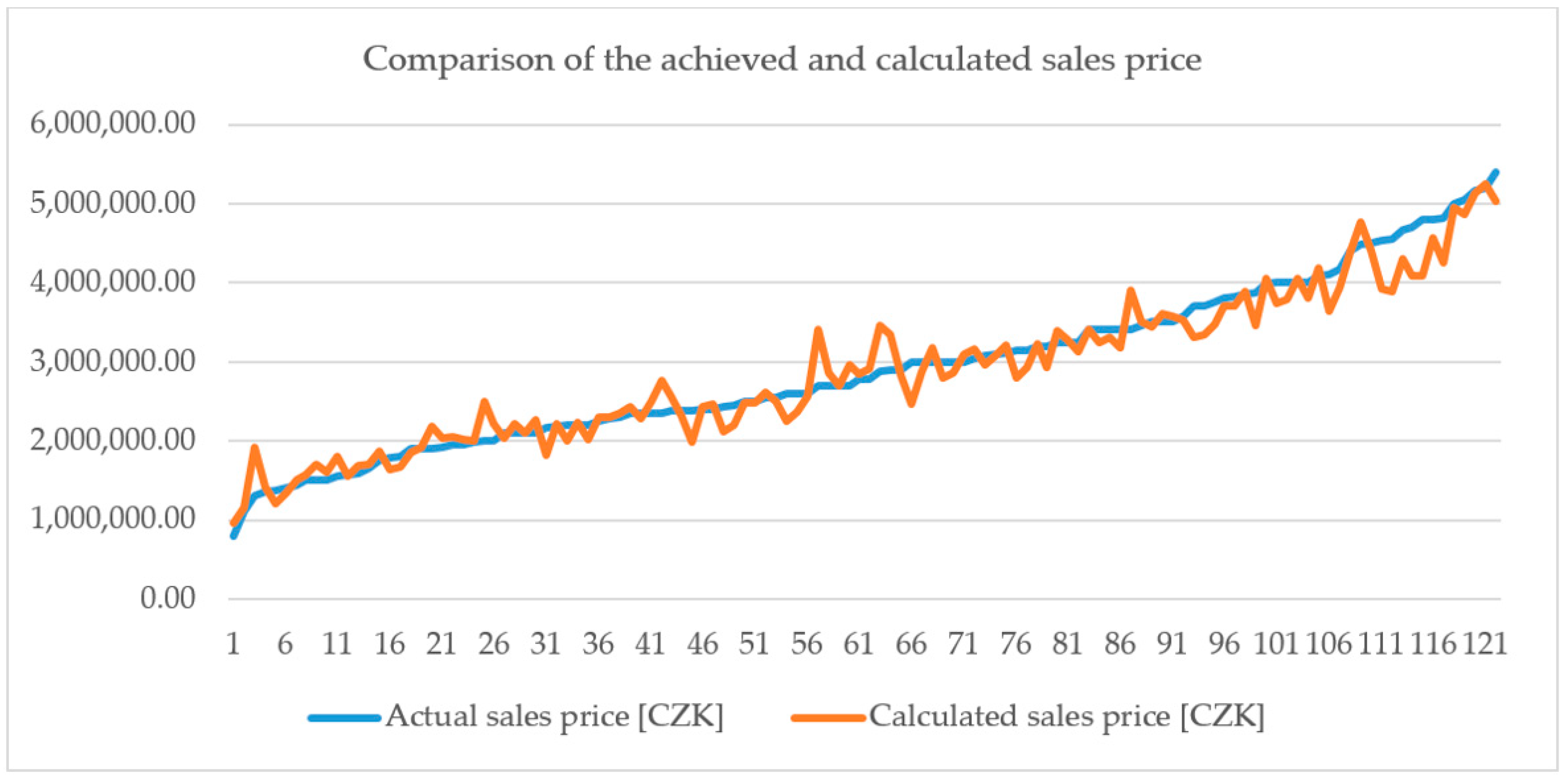
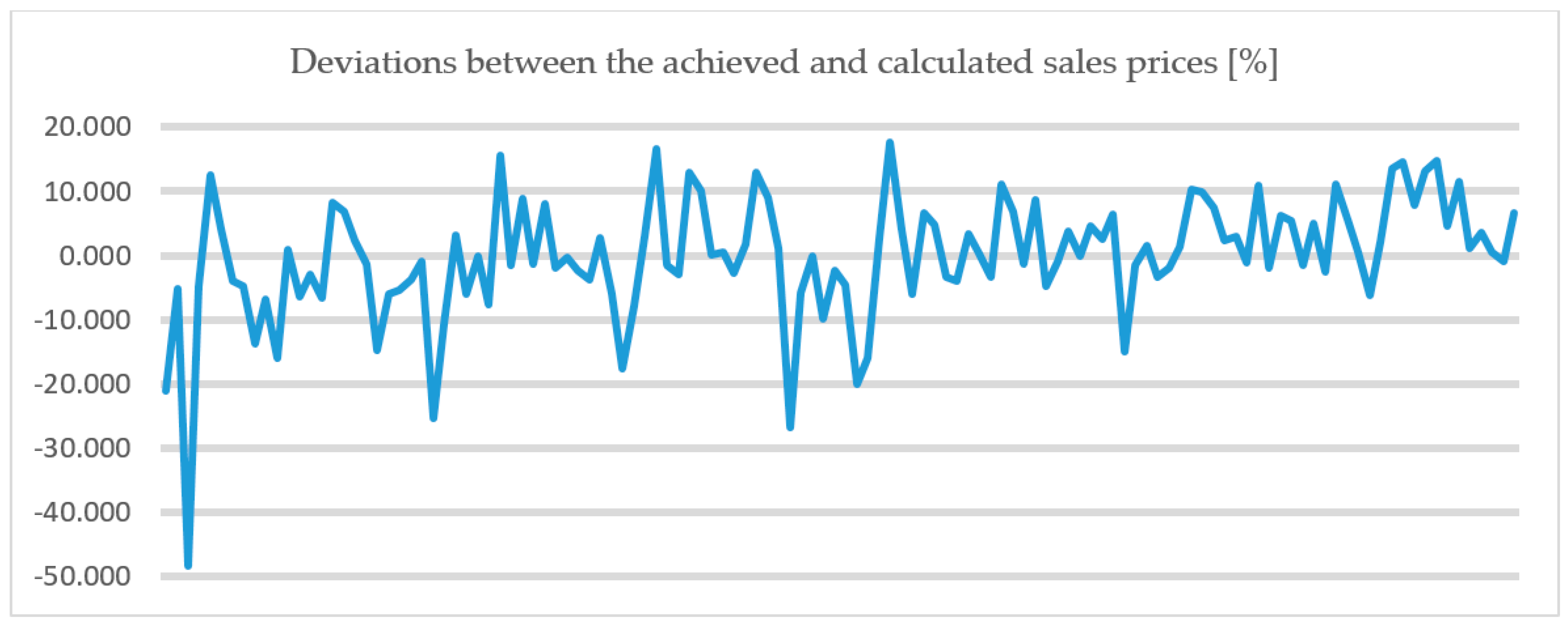
3. Results

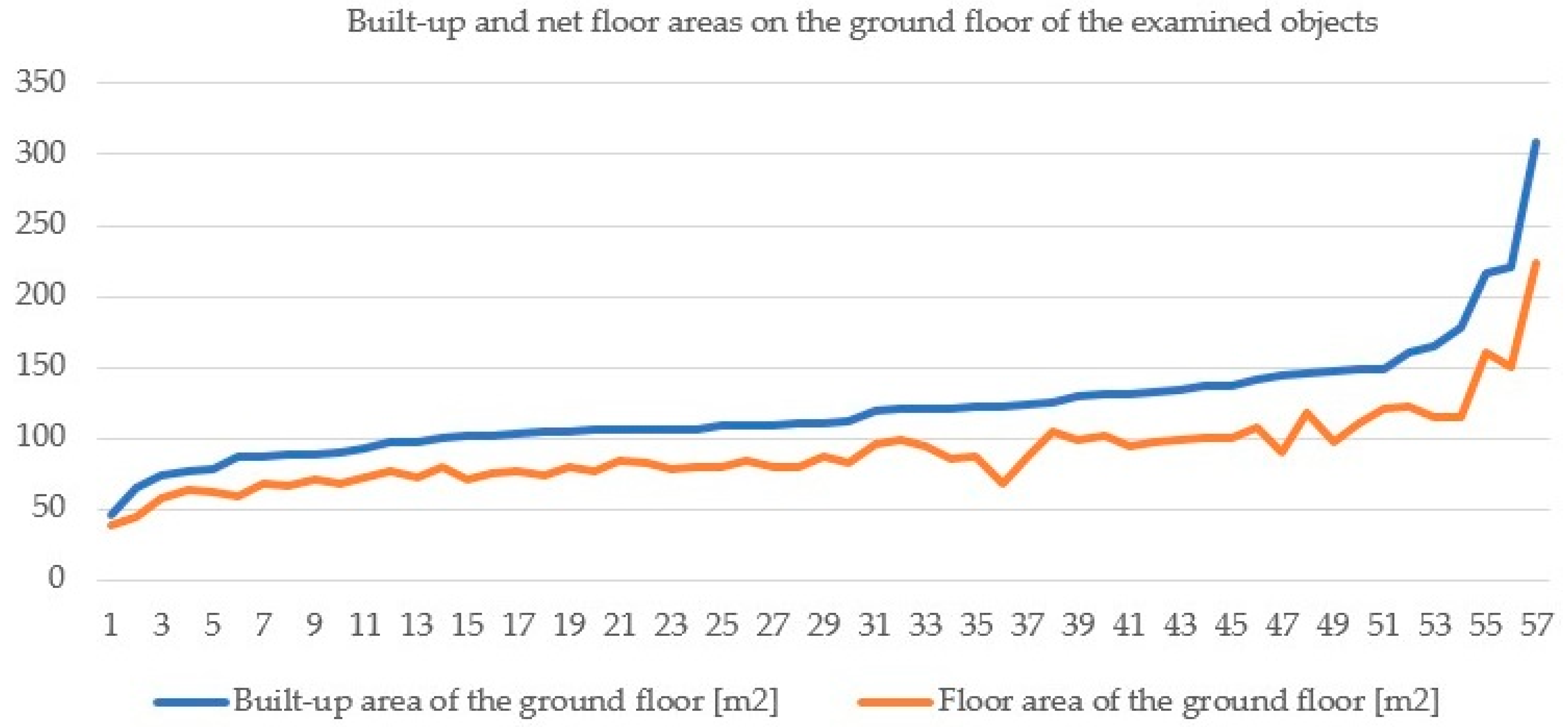
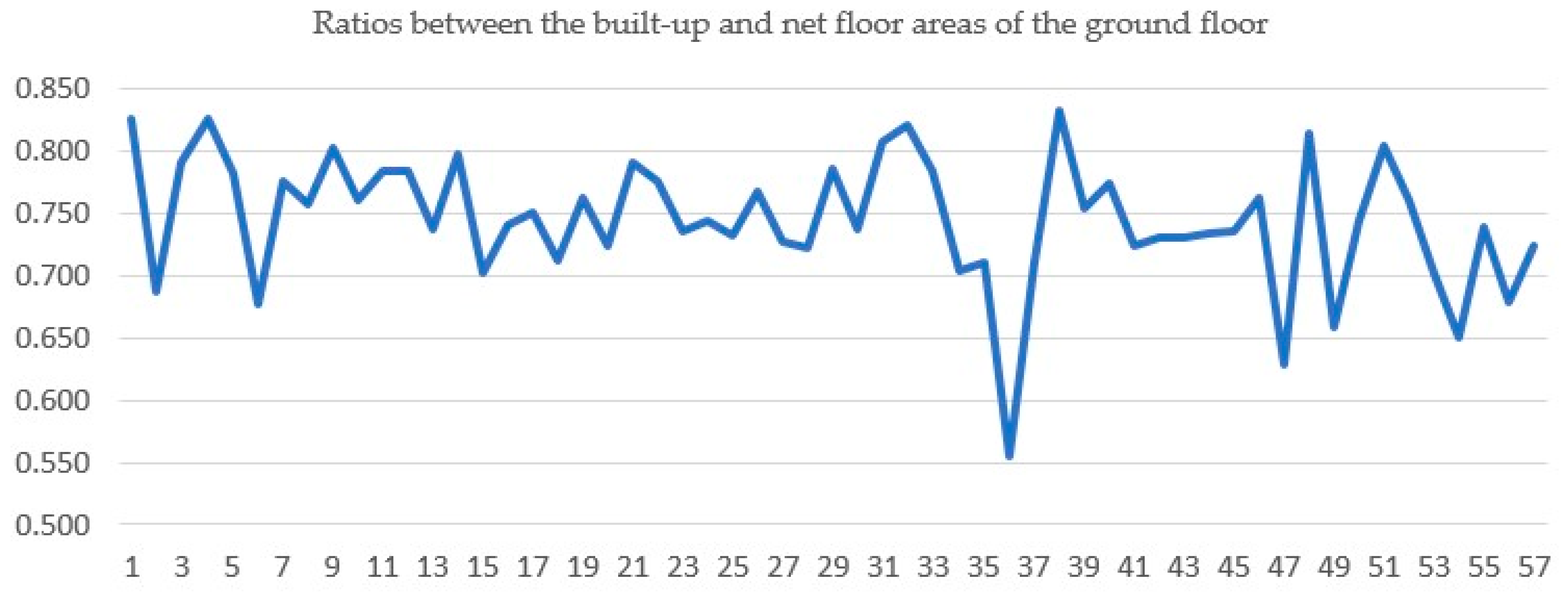
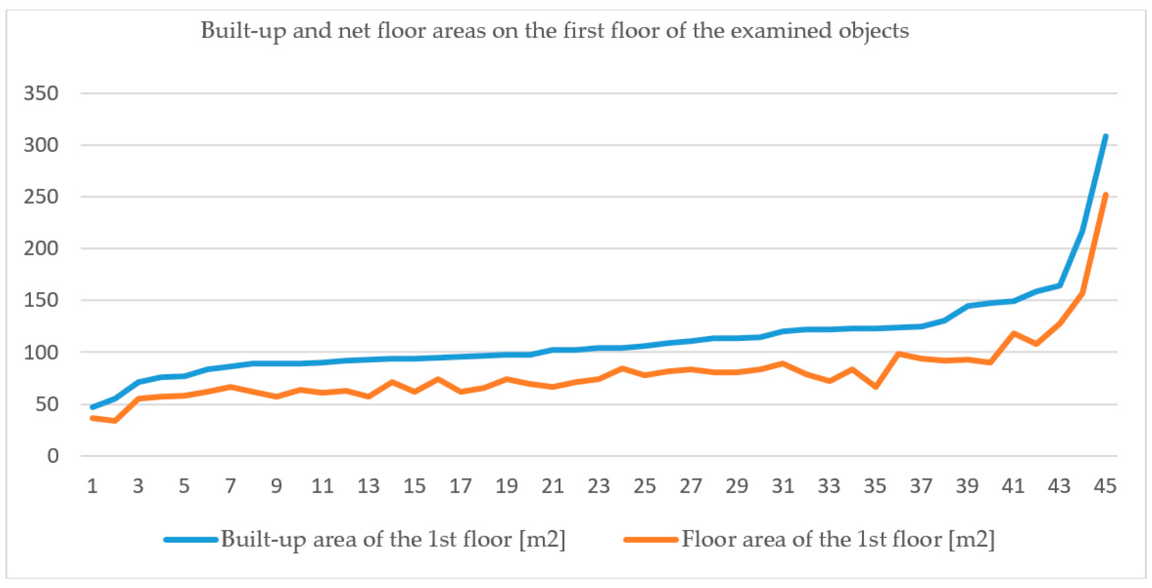
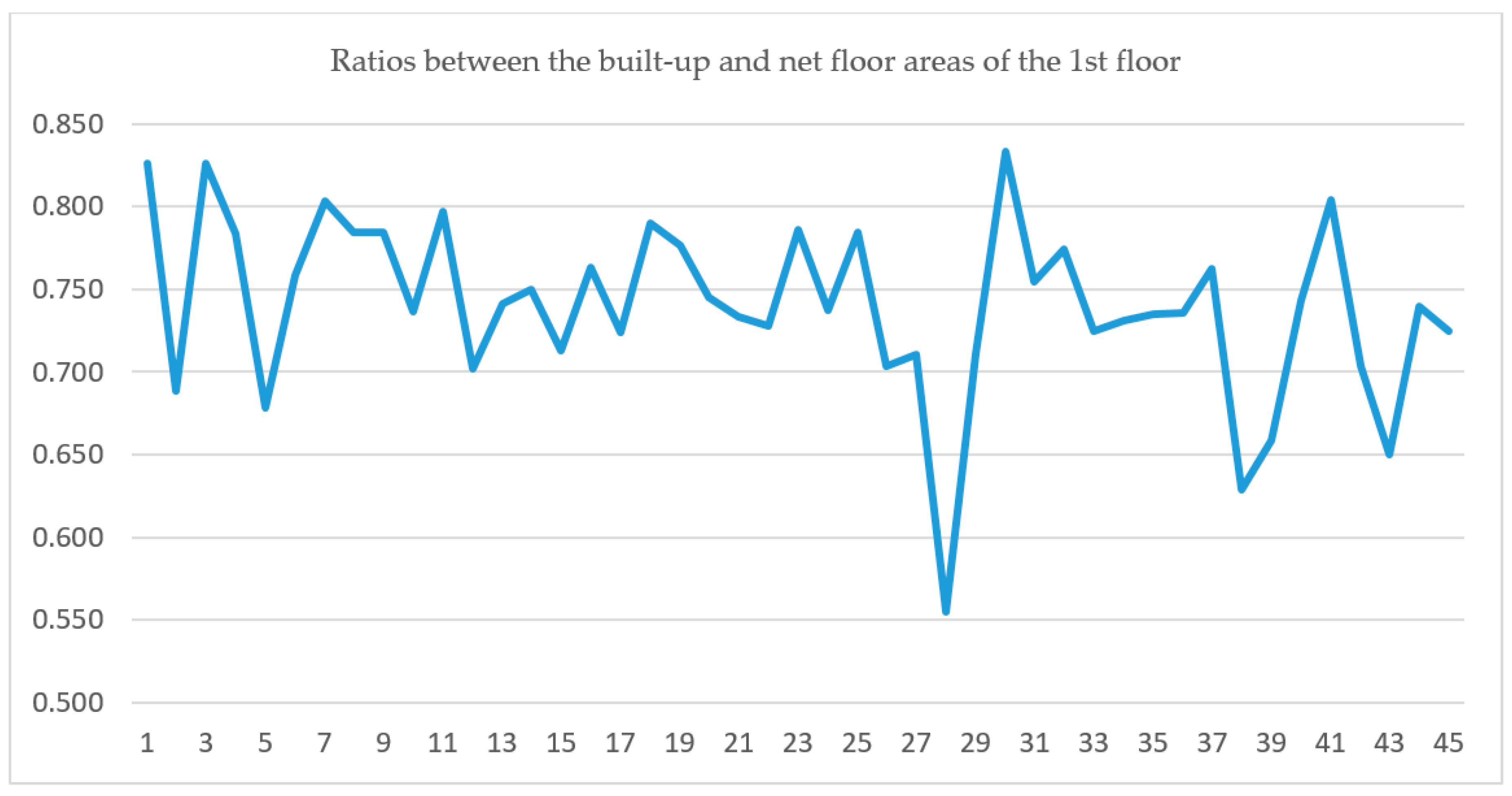
3.1. The Relationship between the Built-Up and Net Floor Areas of Detached Houses

Data about 57 real objects were collected in order to determine the ratio between the built-up and net floor areas of detached houses. These detached houses were personally visited by the authors and, in all cases, they used a laser distance meter to measure both the built-up and net floor areas of individual floors. The structures were placed in order from largest to smallest.
Figure 1 shows the built-up areas and net floor areas of individual structures. Figure 2 shows the ratios between the built-up and net floor areas. These all concern the ground floor. Figure 3 and Figure 4 below show the same, with the difference that these data apply to the first floor, or possibly the attic. Houses that have only one floor—a total of 12 samples—were therefore eliminated from the examined samples in the second case. In the case of houses with a saddle roof, the angled ceilings of the attics are not taken into consideration—the floor areas were measured from the interior faces of the vertical load-bearing structures.
Figure 1, Figure 2, Figure 3 and Figure 4 indicate several facts:
  • It is evident that most of the values of the examined ratios fall within an interval between 0.70 and 0.80.
  • Greater deviations only apply to single cases; with regard to the numbers, there are slightly more cases where the examined ratio is less than 0.70.
  • Houses with a built-up area ranging from 90 to 120 square meters have the most stable examined ratio; the values of houses with a built-up area outside this range deviate much more.
During investigation of specific structures that have extreme values of the aforementioned ratio, it was found that structures in which the age of the main load-bearing structures is 100 or more years achieve the local minimum. Different procedures were used during this period; it was particularly common for the main load-bearing structures to be much more massive, especially in order to maintain a comfortable interior temperature [40]. On the contrary, local maximums are displayed by new builds, particularly by wood-builds using sandwich technology, the load-bearing structures of which are very lightly built. The basic statistics of the aforementioned data are evident from Table 1.
The above indicates that the total net floor area can be determined fairly accurately for all detached houses by multiplying the built-up area by a coefficient ranging from 0.75 to 0.80. The determinant deviation in this case is very low. In the case of old houses with massive structures, this coefficient should be reduced down to the value of 0.60; on the contrary, this value should be around 0.80 for new builds.

3.2. Determining the Values of Coefficients

The potential for utilization of the formula must be practically verified. As stated by Kettani [41], when determining the values, the assessed real estate must be compared to other assets of very similar size and location—the market needs to be segmented. The segment of detached houses that may have a cellar or have a single floor with an occupied attic—or those that have a saddle roof, where the attic area is partially restricted as a result of the angle of the ceiling—was chosen to demonstrate the potential to establish the values of the aforementioned coefficients. The plot size of detached houses that were included in the selection was limited to a maximum of 1500 square meters—if the area of the plot was larger, this could mean that economies of scale would have a significant impact on the unit value of the land plot, which would distort the results. A total of 122 sales of detached houses in the city of Ostrava and its surrounding area were analyzed. The data were chosen from a database of actually sold real estate—this database includes photographs of individual assets, a brief description, and the development of the offered sales price until the time the house was sold [42].
The Czech State Administration of Land Surveying and Cadaster [43] has registered actual sales prices in the Czech Republic since 2014. It acquires these data from the sales contracts submitted to it. These data are subsequently publicly available, but for a fee. In the case of the examined sample of sales, the usual local value of the plot was deducted from the total sales price, which gave us the value of the structure itself. The size of the built-up area of the individual floors was subsequently measured in the cadastral map; this was multiplied by a coefficient of 0.75—see above—which resulted in the approximate net floor area of the individual floors. The degree of wear of each structure and the coefficient taking into consideration changes to price over time—see above—were also determined.
Basic statistical descriptive data of the investigated quantities are given in Table 2 and Table 3. The statistics of cellars floor areas and attics do not include houses that do not have these parts.
Standard multiple regression using the ordinary least squares method was used to obtain the values of the required coefficients from the obtained data. These values are as follows:
  • β1 = 336.59,
  • β2 = 35,500.09,
  • β3 = 19,847.12.
If we enter the values of the aforementioned coefficients into formulas (3), (4), and (5), we obtain coefficients α1 and α3:
  • α1 = 0.009,
  • α3 = 0.559.
The basic descriptive outputs of the performed multiple regression analysis are given in Table 4.
The correlation coefficient and the correlation determination show a very strong dependence between the floor area of the structure and the total price, which is, however, quite evident and expected. However, the fact that the floor area of the cellar has a very minimal influence on the total price of the house is a surprising finding. This means that whether the specific object has a cellar or not is quite insignificant to the buyer.
The smaller influence of the floor area of the attic is also evident from the results. In other words, if two houses with the same floor area are sold, although one of them has a single, ground floor and the other has a ground floor with an occupied attic, the bungalow will be sold for a higher price. This is caused by the fact that only houses with a saddle roof were chosen for the analysis, where utilization of attic areas is limited by the angle of the roof, and also by people’s general unwillingness to walk up and down stairs [44].
It is also evident from the values of the created coefficients that the unit sales prices of newly built houses (i.e., objects with zero wear) are around 35,000 CZK/square meter. In the authors’ experience, this corresponds to factual prices; the aforementioned amount is also very close to construction costs.
To verify the overall significance of the performed analysis, a complete F-test of the entire data set was performed. In this case:
F significance = 6.2 × 10−107,
which is a value much lower than the commonly required levels of significance, so the chosen model can be described as very significant.
There are two more graphs included for better interpretation of the results. Figure 5 shows a comparison between the realized sales prices of detached houses and the prices that were calculated by entering all the values into formula (7). Figure 6 shows the percentage deviations between the achieved and calculated prices in individual cases. The transactions were placed in ascending order according to actual price.
Figure 5 and Figure 6 indicate that the aforementioned method can be used to determine the price of a detached house with a maximum deviation of 20%. However, we can see three cases here where the achieved deviation is negative and higher than 20%. This means that these three houses were sold for a significantly lower price than that corresponding to the market conditions. This can be explained by the sellers’ efforts to sell the house as soon as possible and have the money from the sale very soon (e.g., due to an urgent or difficult situation). However, as can be seen from the above, this concerns individual exceptions.
It is also clear from Figure 6 that the more expensive the house, the lower the deviation between the achieved and calculated sales prices, which is up to 10% in most cases of newer houses. This is particularly because the most expensive houses are also the newest, and it is easier to determine objective wear (mostly using linear methods). If the houses are older, the essential age of some structures can only be estimated, which distorts the degree of wear, and this distortion is reflected in the calculation.

4. Discussion

The aforementioned method can be used to automate the valuation of detached houses. However, the analysis must always be performed for a specific segment of detached houses only. A regression analysis can be performed to obtain the values of the coefficients necessary for calculation of the price, and these can be entered into the system; then, the user simply gives the data that can be obtained from public sources when establishing the market value of a specific detached house. Alternatively, these data may be specified by the owner of the assessed real estate themselves—the area of the plot, the usual price of a plot in that location, the floor areas of individual floors, and the estimated degree of wear. With the exception of a few cases, the deviation between the aforementioned calculation and the actual market price of the real estate ranges up to 20%, and up to 10% in approximately 80% of cases. This means that the price can be calculated quite accurately. This method also does not depend very much on the valuer’s subjective opinion. If the β coefficients can also be determined for other types of detached houses and, possibly, for other types of assets, a system can be created that can be used to determine the market values of detached houses with very small deviations. This system could then be used, for example, for tax purposes.
Although the mentioned methodology was conceived and researched in the Czech environment, it would be beneficial to verify its applicability in other European countries through further research. Its main advantage is the overall simplicity and practical comprehensibility, even for people moving outside the real estate market. Other automated systems are very sophisticated, but they also provide more accurate results; on the other hand, they may be too difficult for many users. It is even possible that some data that are necessary for valuation are not available at all—e.g., data on the number of bedrooms, orientation of living rooms, number of balconies, etc. are not a common part of statistical data of realized real estate transactions in the Czech Republic. In addition, the vast majority of foreign automated models are focused only on apartments; the method presented here shows a possible method of house valuation, and thus contributes to the overall transparency of the real estate market, which undoubtedly affects the overall sustainability of the territory as a whole.
However, the aforementioned method can also be considered a method for establishing the usual value of land in a specific location if data about the actual sale of plots in that specific location are not available, but where detached houses are often sold—typically in densely developed areas with a shortage of vacant plots.
Further research in this field should focus on establishing the values of the relevant coefficients for other types of detached houses, or could possibly be used to verify whether the aforementioned method may also be applicable to other types of structures (e.g., retail units, manufacturing sheds, etc.) or in other countries. A more objectivized method of calculating wear, particularly in relation to older structures, would also be beneficial.

Author Contributions

S.E. provided the core idea, collected the data and wrote the manuscript. M.T. analyzed the data statistically. D.K. revised and constructively commented on the paper, checked the formal correctness. All authors have read and agreed to the published version of the manuscript.

Funding

This research received no external funding.

Acknowledgments

This work was supported by funds for the Conceptual Development of Science of the VSB—Technical University of Ostrava, Research and Innovation for 2020.

Conflicts of Interest

The authors declare no conflict of interest.

References

  1. Renigier-Bilozor, M.; Janowski, A.; d’Amato, M. Automated valuation model based on fuzzy and rough set theory for real estate market with insufficient source data. Land Use Policy 2019, 87. [Google Scholar] [CrossRef]
  2. Arribas, I.; Garcia, F.; Guijaro, F.; Oliver, J.; Tamosiuniene, R. Mass appraisal of residential real estate using multilevel modelling. Int. J. Strateg. Prop. Manag. 2016, 20, 77–87. [Google Scholar] [CrossRef] [Green Version]
  3. Özdilek, Ű. On Price, Cost, and Value. Apprais. J. 2010, 78, 71–79. [Google Scholar]
  4. Bailey, M.J.; Muth, R.F.; Nourse, H.O. A regression method for real estate price index construction. J. Am. Stat. Assoc. 1963, 58, 933–942. [Google Scholar] [CrossRef]
  5. Graaskamp, J.; Robbins, M. Business 868 Lecture Notes; University of Wisconsin: Madison, WI, USA, 1987. [Google Scholar]
  6. Doumpos, M.; Papastamos, D.; Andritsos, D.; Zopounidis, C. Developing automated valuation models for estimating property values: A comparison of global and locally weighted approaches. Ann. Oper. Res. 2020. [Google Scholar] [CrossRef]
  7. Bitter, C.; Mulligan, G.F.; Dall’erba, S. Incorporating spatial variation in housing attribute prices: A comparison of geographically weighted regression and the spatial expansion method. J. Geogr. Syst. 2007, 9, 7–27. [Google Scholar] [CrossRef] [Green Version]
  8. Füss, R.; Koller, J.A. The role of spatial and temporal structure for residential rent predictions. Int. J. Forecast. 2016, 32, 1352–1368. [Google Scholar] [CrossRef]
  9. Yunjong, K.; Seungwoo, C.; Mun, Y.Y. Applying Comparable Sales Method to the Automated Estimation of Real Estate Prices. Sustainability 2020, 12, 5679. [Google Scholar]
  10. Shehata, W.; Abu Arqoub, M.; Langston, C. From hard bed to luxury home: Impacts of reusing HM Prison Pentridge on property values. J. Hous. Built Environ. 2020. [Google Scholar] [CrossRef]
  11. Corcoran, C.; Liu, F. Accuracy of Zillow’s home value estimates. Real Estate Issues 2014, 39, 45–49. [Google Scholar]
  12. Du, M.; Zhang, X. Urban greening: A new paradox of economic or social sustainability? Land Use Policy 2020, 92, 104487. [Google Scholar] [CrossRef]
  13. Jim, C.Y.; Chen, W.Y. Impacts of urban environmental elements on residential housing prices in Guangzhou (China). Landsc. Urban Plan. 2006, 78, 422–434. [Google Scholar] [CrossRef]
  14. Case, B.; Clapp, J.; Dubin, R.; Rodriguez, M. Modelling spatial and temporal house price patterns: A comparison of four models. J. Real Estate Financ. Econ. 2004, 29, 167–191. [Google Scholar] [CrossRef]
  15. Pace, R.; Gilley, O. Generalizing the OLS and grid estimators. Real Estate Econ. 1998, 1, 331–346. [Google Scholar] [CrossRef]
  16. Bourassa, S.; Cantoni, E.; Hoesli, M. Predicting house prices with spatial dependence: A comparison of alternative methods. J. Real Estate Res. 2010, 32, 139–159. [Google Scholar]
  17. Ciuna, M.; De Ruggiero, M.; Salvo, F.; Simonotti, M. Automated Procedures Based on Market Comparison Approach in Italy. In Advances in Automated Valuation Modeling. Studies in Systems, Decision and Control; d’Amato, M., Kauko, T., Eds.; Springer: Cham, Germany, 2017; Volume 86, pp. 381–400. [Google Scholar]
  18. Ciuna, M.; Salvo, F.; Simonotti, M. An Estimative Model of Automated Valuation Method in Italy. In Advances in Automated Valuation Modeling. Studies in Systems, Decision and Control; d’Amato, M., Kauko, T., Eds.; Springer: Cham, Germany, 2017; Volume 86, pp. 85–112. [Google Scholar]
  19. Morano, P.; Tajani, F.; Locurcio, M. Multicriteria analysis and genetic algorithms for mass appraisals in the Italian property market. Int. J. Hous. Mark. Anal. 2018, 11, 229–262. [Google Scholar] [CrossRef]
  20. Mothorpe, C.C.; Wyman, D.M. The appraisal of residential water view properties. Apprais. J. 2017, 85, 130–141. [Google Scholar]
  21. Lan, F.; Wu, Q.; Zhou, T.; Da, H. Spatial Effects of Public Service Facilities Accessibility on Housing Prices: A Case Study of Xi’an, China. Sustainability 2018, 10, 4503. [Google Scholar] [CrossRef] [Green Version]
  22. Diao, M.; Zhu, Y.; Zhu, J. Intra-city access to inter-city transport nodes: The implications of high-speed-rail station locations for the urban development of Chinese cities. Urban Stud. 2017, 54, 2249–2267. [Google Scholar] [CrossRef]
  23. Xue, C.; Ju, Y.; Li, S.; Zhou, Q. Research on the Sustainable Development of Urban Housing Price Based on Transport Accessibility: A Case Study of Xi’an, China. Sustainability 2020, 12, 1497. [Google Scholar] [CrossRef] [Green Version]
  24. Morancho, A.B. A hedonic valuation of urban green areas. Landsc. Urban Plan. 2003, 66, 35–41. [Google Scholar] [CrossRef]
  25. Park, J.H.; Lee, D.K.; Park, C.; Kim, H.G.; Jung, T.Y.; Kim, S. Park accessibility impacts housing prices in Seoul. Sustainability 2017, 9, 185. [Google Scholar] [CrossRef] [Green Version]
  26. Bond, S. HVOTLs in New Zealand. In Towers, Turbines and Transmission Lines: Impacts on Property Value; Wiley Publishing: Hoboken, NJ, USA, 2013; pp. 81–99. [Google Scholar]
  27. Endah, S. Impact of air pollution on property values: A hedonic price study. J. Ekon. Pembang. Kaji. Masal. Ekon. Dan Pembang. 2013, 14, 52–65. [Google Scholar]
  28. Simons, R.A.; Saginor, J.D. A meta-analysis of the effect of environmental contamination and positive amenities on residential real estate values. Real Estate Res. 2006, 28, 71–104. [Google Scholar]
  29. Broome, R. The stigma of Pentridge the view from Coburg 1850–1987. J. Aust. Stud. 1988, 12, 3–18. [Google Scholar] [CrossRef]
  30. Fik, T.J.; Ling, D.C.; Mulligan, G.F. Modelling spatial variation in housing prices: A variable interaction approach. Real Estate Econ. 2003, 31, 623–646. [Google Scholar] [CrossRef]
  31. Bourassa, S.C.; Hoesli, M.; Peng, V.S. Do housing submarkets really matter? J. Hous. Econ. 2003, 12, 12–28. [Google Scholar] [CrossRef] [Green Version]
  32. Kucharska-Stasiak, E. Uncertainty of property valuation as a subject of academic research. Real Estate Manag. Valuat. 2013, 21, 17–25. [Google Scholar] [CrossRef] [Green Version]
  33. Baraňska, A. Real Estate Mass Appraisal in Selected Countries—Functioning Systems and Proposed Solutions. Real Estate Manag. Valuat. 2013, 21, 35–42. [Google Scholar] [CrossRef] [Green Version]
  34. Kuta, V.; Endel, S. Bydlení v Souvislostech [Housing in Context]; VSB—Technical University of Ostrava: Ostrava, Czech Republic, 2018. [Google Scholar]
  35. Himmelberg, C.; Mayer, C.; Sinai, T. Assessing high house prices: Bubbles, fundamentals and misperceptions. J. Econ. Perspect. 2005, 19, 67–92. [Google Scholar] [CrossRef] [Green Version]
  36. Bradáč, A. Teorie a Praxe Oceňování Nemovitých Věcí [Theory and Practice of Real Estate Valuation]; Akademické Nakladatelství CERM, s.r.o.: Brno, Czech Republic, 2016. [Google Scholar]
  37. Reichert, A.K. The impact of interest rates, income, and employment upon regional housing prices. J. Real Estate Financ. Econ. 1990, 3, 373–391. [Google Scholar] [CrossRef]
  38. Oust, A.; Hansen, S.N.; Pettrem, T.R. Combining Property Price Predictions from Repeat Sales and Spatially Enhanced Hedonic Regressions. J. Real Estate Financ. Econ. 2020, 61, 183–207. [Google Scholar] [CrossRef] [Green Version]
  39. Český Statistický Úřad [Czech Statistical Office]. Ceny Sledovaných Druhů Nemovitostí [Prices of Monitored Types of Real Estate]. 2019. Available online: www.czso.cz (accessed on 14 May 2020).
  40. Konstantinov, A.; Mukhin, A. Providing thermal protection when replacing window blocks in historical buildings. In Proceedings of the 3rd International Conference on Sustainable Cities, Moscow, Russia, 18 May 2018. [Google Scholar]
  41. Kettani, O.; Oral, M. Designing and implementing a real estate appraisal system: The case of Quebec Province, Canada. Socio-Econ. Plan. Sci. 2015, 49, 1–9. [Google Scholar] [CrossRef]
  42. INEM. Ucelený Přehled o Bydlení a Životních Podmínkách [A Comprehensive Overview of Housing and Living Conditions]. 2020. Available online: www.inem.cz (accessed on 24 May 2020).
  43. Český Úřad Zeměměřičský a Katastrální [Czech Cadastre of Real Estate]. Státní Správa Zeměměřičství a Katastru [State Administration of Land Surveying and Cadastre]. 2020. Available online: www.cuzk.cz (accessed on 22 May 2020).
  44. Gehl, J. Cities for People; Island Press: Washington, DC, USA, 2013. [Google Scholar]
Figure 1. Built-up and net floor areas of the ground floors of individual objects.
Sustainability 12 07774 g001
Figure 2. Ratios between the built-up and net floor areas of the ground floors of a sample of houses.
Sustainability 12 07774 g002
Figure 3. Built-up and net floor areas of the first floors of individual structures.
Sustainability 12 07774 g003
Figure 4. Ratios between the built-up and net floor areas of the first floors of a sample of houses.
Sustainability 12 07774 g004
Figure 5. Comparison of the achieved and calculated prices of detached houses.
Sustainability 12 07774 g005
Figure 6. Deviations between the achieved and calculated prices of detached houses.
Sustainability 12 07774 g006
Table 1. Basic statistics of the set of data of the examined ratios.
Ratio between Built-Up and Net Floor Areas on the Ground Floors of all HousesRatio between Built-Up and Net Floor Areas on the First Floors of all Houses
No. of samples5745
Maximum0.8330.868
Minimum0.5550.601
Average0.7460.764
Median0.7440.769
Determinant deviation0.0520.065
Table 2. Basic statistics of the set of data of the examined prices.
Total Sales Prices (CZK)Plot Sizes (Square Meters)Local Usual Values of the Plots (CZK)
No. of samples122122122
Maximum5,390,00014992600
Minimum799,000192155
Average2,917,6898041202
Median2,780,0008041200
Determinant deviation1,031,117306538
Table 3. Basic statistics of the set of data of the examined floor area and wear.
Cellar Floor Area (Square Meters)Floor Area of Ground Floor (Square Meters)Floor Area of Attic (Square Meters)Wear (%)
No. of samples95122113122
Maximum1261269780
Minimum2038105
Average69815744
Median74796045
Determinant deviation22172220
Table 4. Basic descriptive outputs of the performed regression analysis.
Correlation coefficient R0.992268
Correlation determination R20.984596
CoefficientsMedian Value ErrorValue tValue p
Cellar floor area336.591309.1570.2571031290.797543181
Floor area of ground floor35,500.091258.89428.199415921.607 × 10−54
Floor area of attic19,847.12158312.537661611682 × 10−23

