Article

Machine Learning for Conservation Planning in a Changing Climate

by
Ana Cristina Mosebo Fernandes
,
Rebeca Quintero Gonzalez
,
Marie Ann Lenihan-Clarke
,
Ezra Francis Leslie Trotter
and
Jamal Jokar Arsanjani
*
Department of Planning, Geography and Surveying, Aalborg University Copenhagen, A.C Meyers Vænge 15, 2450 Copenhagen, Denmark
*
Author to whom correspondence should be addressed.
Sustainability 2020, 12(18), 7657; https://doi.org/10.3390/su12187657
Submission received: 21 July 2020 / Revised: 31 August 2020 / Accepted: 12 September 2020 / Published: 16 September 2020

Abstract

:
Wildlife species’ habitats throughout North America are subject to direct and indirect consequences of climate change. Vulnerability assessments for the Intermountain West regard wildlife and vegetation and their disturbance as two key resource areas in terms of ecosystems when considering climate change issues. Despite the adaptability potential of certain wildlife, increased temperature estimates of 1.67–2 °C by 2050 increase the likelihood and severity of droughts, floods, heatwaves and wildfires in Utah. As a consequence, resilient flora and fauna could be displaced. The aim of this study was to locate areas of habitat for an exemplary species, i.e., sage-grouse, based on current climate conditions and pinpoint areas of future habitat based on climate projections. The locations of wildlife were collected from Volunteered Geographic Information (VGI) observations in addition to normal temperature and precipitation, vegetation cover and other ecosystem-related data. Four machine learning algorithms were then used to locate the current sites of wildlife habitats and predict suitable future sites where wildlife would likely relocate to, dependent on the effects of climate change and based on a timeframe of scientifically backed temperature-increase estimates. Our findings show that Random Forest outperforms other competing models, with an accuracy of 0.897, and a sensitivity and specificity of 0.917 and 0.885, respectively, and has great potential in Species Distribution Modeling (SDM), which can provide useful insights into habitat predictions. Based on this model, our predictions show that sage-grouse habitats in Utah will continue to decrease over the coming years due to climate change, producing a highly fragmented habitat and causing a loss of close to 70% of their current habitat. Priority Areas of Conservation (PACs) and protected areas might be deemed insufficient to halt this habitat loss, and more effort should be put into maintaining connectivity between patches to ensure the movement and genetic diversity within the sage-grouse population. The underlying data-driven methodical approach of this study could be useful for environmentalists, researchers, decision-makers, and policymakers, among others.

1. Introduction

Wildlife conservation brings balance and value to ecological systems, supported by the environmental ethics of biocentrism. As a practice, conservation is of growing importance due to the role that nature plays in mitigating the negative impacts of global warming through its ability to regulate climate change [1]. According to the Convention on Biological Diversity (CBD), it is of the uttermost importance to ensure: (a) the conservation of biological diversity, (b) the sustainable use of the components of biological diversity and (c) the fair and equitable sharing of the benefits arising from the utilization of genetic resources [2]. Due to human activities in general, many ecosystems are being destroyed or damaged, and we are facing a massive extinction of most kinds of species.
This loss of ecosystems will seriously aggravate the climate situation, which will, in turn, negatively impact the remaining ecosystems and wildlife. Through this feedback, environmental changes will happen faster the worse the situation gets, accelerating the effects of climate change and ecosystem degradation. To stop this feedback and decelerate or even stop ecosystem degradation and biodiversity loss, the United Nations (UN) has set some Sustainable Development Goals (SDGs) that are to be met in order to avoid reaching any tipping points [3]. The urgency associated with mitigating the harmful consequences in connection to climate change incites the use of innovative techniques and tools. Species Distribution Models (SDMs) are one such tool that use observation data in conjunction with environmental variables to project the presence or absence of a species both spatially and temporally [4], ultimately assisting in conservation efforts.
Machine learning (ML) is also playing a crucial role in bridging a gap between computer science and biology in demonstrating its utility as an advantageous component of species distribution modeling. By automating time-consuming processes, ML overcomes the challenges presented to us from non-linear, high-dimensional data and continues to grow in popularity. This is also, in part, due to its ability to cope with the scarcity of absence data and making use of the abundance of presence data that are available for countless wildlife species [5].
The region of Utah is particularly vulnerable to the effects of climate change, mainly due to the semi-arid nature of the region [6]. Its wildlife is equally sensitive to climate change effects, including 42 endangered species and 166 sensitive species of both flora and fauna [7]. The impacts of climate change on the environment have both direct and indirect consequences on wildlife habitats and food sources, leading to the wildlife’s inevitable relocation or potential extinction. Terrestrial ecosystems composed of wetlands, forests, alpine areas and deserts play a vital role in absorbing, storing and managing carbon and water, and therefore, their conservation and restoration are both critical and cost-effective in terms of climate change mitigation and wildlife conservation. Should these areas not be preserved, and feedback loops occur, lands will convert from carbon sinks to carbon sources [1]. In the western states, where the study area for this study is located, this will translate to a decrease in ecosystem resilience, a diminished water supply, an increase in vulnerability to drought and a susceptibility to damage caused by wildfires [8]. As a result, wildlife habitat fragmentation and loss could occur, which are directly linked to biodiversity loss [9] and could ultimately be the cause of the decline and extinction of many wildlife species [10].
This study seeks to address such wildlife habitat concerns by combining the use of SDMs with ML algorithms to provide supplementary information for strategic conservation planning, which, to date, has been a primarily standalone approach [11]. Traditional methods are still common practice in strategic conservation planning, despite the emergence of ML applications in this area, which make use of the most recent scientific and technological resources. SDMs enable the use of Volunteered Geographic Information (VGI) and open source tools. The context of VGI data lies within citizen science, with it being a form of user-generated content made possible by technological advances. Both VGI and open source tools allow for the incorporation of many ML algorithms for easy comparison and allow for the assessment of their collective use in terms of reliability, efficiency, accuracy, flexibility and potential as a tool for future habitat modeling. There are a considerable number of studies that focus on these issues, of which some are selected for a comparative summary in Table 1.

1.1. Species Distribution Modeling

Through the combined use of wildlife occurrence data and environmental data, threats that pose a risk to certain species, such as climate change, can be evaluated and appropriate mitigation measures to be taken advocated for. SDMs can not only predict the current location of wildlife presence but are also used for future habitat suitability mapping. This is dependent on projected environmental scenarios using relevant variables [4,15]. SDMs and their value in conservation decision-making and management are subject to certain criticisms and discussion points. To address these and maximize species distribution modeling potential, attention should be paid to the reliability and comprehensiveness of input data, the model should be assessed appropriately, and iterations should be performed for the process until a defensible and reproducible model can be established [11,16].
Observation data are often critiqued for their lack of absence points [13]; the presence points of a species in a study area are confirmed, but no further information regarding the presence or absence of that species is provided for the remainder of the area where no data are available. Therefore, observation data provide insight only into where confirmed sightings of a species occur and, additionally, where we must decide whether bias or other issues may also exist. For example, sightings that are recorded in someone’s garden in an urban area miles from a lek may be considered inaccurate. This criticism for observation-only data can be addressed in one of two following ways: firstly, by using a presence-only model, or secondly, through the creation of pseudo-absences. However, some argue that absence points only confuse the model due to the assumption that all records represent non-habitats when, in fact, they could signify suitable-yet-inaccessible habitats [16]. Furthermore, the overall evaluation of the model’s credibility should be derived from performance-based statistics; studies show that kappa, Area Under the Curve and Receiver Operating Characteristic (AUC-ROC), and correlation coefficients provide relevant and useful information in model analysis.
According to recent research, the ML algorithms most associated with species distribution modelling are Maximum Entropy (MaxEnt), Random Forest (RF), Support Vector Machine (SVM) and Artificial Neural Network (ANN) [4,17]. Each of these algorithms serves to meet the challenge of characterizing the spaces delineating species habitats and categorize the remaining areas depending on whether they meet the same criteria. Each algorithm performs differently when predicting the current and future habitats of sage-grouse, and their results differ in terms of reliability and accuracy, as explained further in Section 4.1. By following a protocol, the combined use of species distribution modelling and ML algorithms can provide predictive results that surpass traditional standalone conservation assessment practices. Through the incorporation of theory, expert opinion and current practice, SDMs could reduce current conservation management real and time-related costs and help to minimize planning errors by providing insight into where future efforts should be focused [18].

1.2. Study Objectives

The purpose of this study is to determine the presence of sage-grouse habitats in the state of Utah based on various ML algorithms, using relevant environmental factors to determine areas of habitat; analyze which algorithms perform best for this task; and, finally, investigate the extent to which these areas will change due to climate change. These locations could then be considered as possible areas of easement for wildlife conservation purposes. Additionally, we seek to investigate the impacts of climate change statewide, predict changes in sage-grouse habitats and infer from the results which areas should be considered for future conservation with respect to wildlife response.

Problem Statement

The state of Utah is making great efforts in wildlife conservation, especially to protect the sage-grouse. However, little is known about the future of this species due to the occurrence of climate change and its impact in this state. Sage-grouse are especially sensitive to these changes due to the fragmented state of their habitats and the already-vulnerable ecosystems that dominate in Utah. With the wide variety of ML algorithms currently in use, it is unknown which of them, whether individually or ensembled with others, performs best in predicting distributions for species restricted in their movements due to fragmented habitats. Hence, this study aims to answer the following research questions:
  • How accurately can sage-grouse habitats be classified using each of the selected ML algorithms based on both continuous and categorical variables?
  • How will sage-grouse habitats in Utah be impacted by the varying future emission scenarios that represent the state’s temperature-change trajectory most closely?
  • Based on the prediction maps for future scenarios obtained from the models, how will the change in sage-grouse habitats affect current conservation areas?

2. Data and Materials
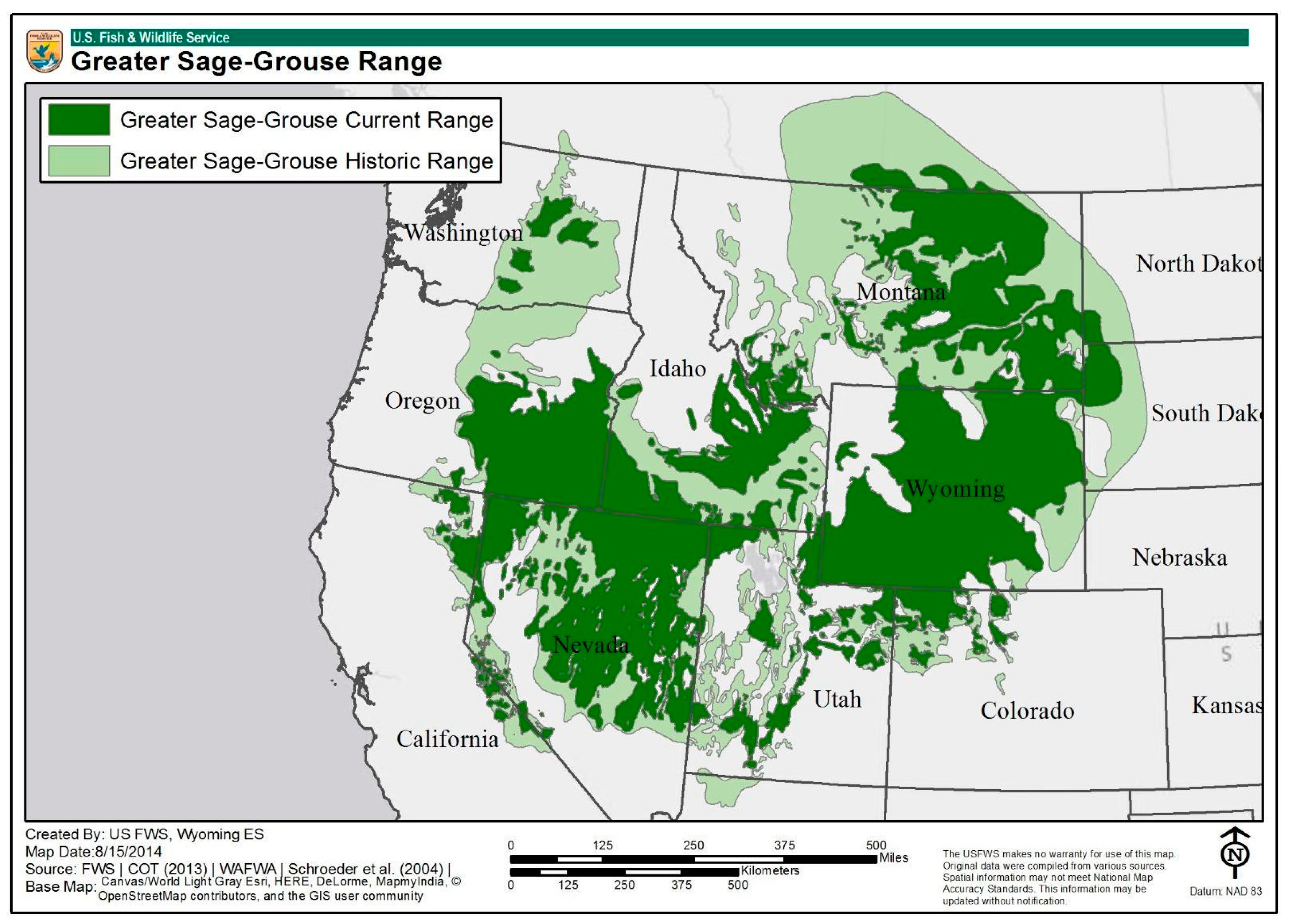
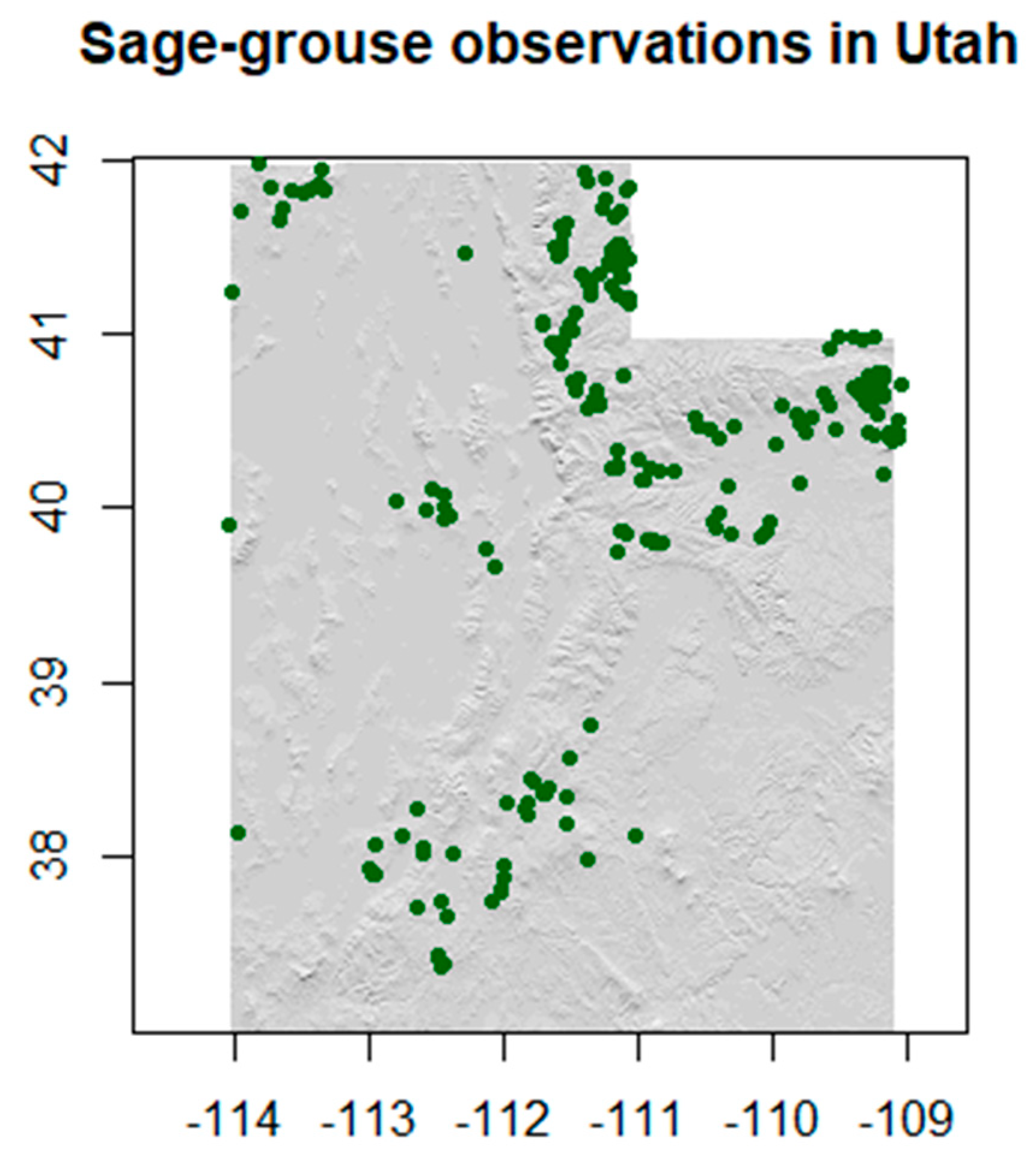
2.1. Study Area

Utah, located in the western United States, is characterized by three major land areas: the Rocky Mountains, the Basin and Ridge region and the Colorado Plateau [19]. Due to the geographical diversity across the state, regions of varying climate persist; however, all are subject to the impacts of climate change [6]. It has been estimated that within the next 30 years, air temperatures will rise by 1.67–2 °C in the summer months. This will result in a higher number of extreme weather events; for instance, a 1.67 °C rise in the average temperature will increase the frequency of droughts in Utah by 2500% [20]. These looming issues have resulted in the State’s necessity for, and implementation of, wildlife conservation efforts. The average yearly investment in state conservation between 1998 and 2005 was USD 13,086,461, and it is evident from its ranking of fifth in the United States for the number of species found in Utah and nowhere else worldwide that safeguarding wildlife habitats will continue to rally support [21].
Other local initiatives to prevent the negative effects of climate change are also underway in certain areas of Utah; for example, carbon sequestration has become a local government talking point in Park City, and strong emphasis has been placed on tracking community progress towards carbon neutrality [22]. Utah’s educational institutions, global-scale businesses, non-profits and political activists are also raising dollars and voices to support such initiatives and protect the nature that contributes to its ecological significance.
The selection and size of the study area are also appropriate due to statewide-conserved lands for which other organizations’ modeling of sage-grouse habitats and Priority Areas of Conservation (PACs) have been established, acting as a comparison for our results. Approximately three quarters of the land in Utah is owned by government entities such as the Bureau of Land Management (BLM), State of Utah Department of Natural Resources (DNR), US National Park Service (NPS), US Forest Service (USFS) and US Fish and Wildlife Service (USFWS/FWS). This does not, however, imply that all such land is protected. Land that is publicly accessible for recreational purposes can also pose its own threats to wildlife habitats, especially when unmanaged.

2.2. Species of Interest: Greater Sage-Grouse (Centrocercus urophasianus)

Despite approximately 75% of Utah’s land being state owned, 34% (3.6 million acres) of the state’s sage-grouse population currently occupies habitats found on private property [23] and collectively inhabits only 56% of its historical range (Figure 1)—a drop from 297 million to 165 million acres in the area occupied [24]. This indicates the importance of continued conservation efforts to preserve and protect sage-grouse habitats by way of easements.
Utah’s sightings of sage-grouse provide the southernmost observations of the species and, according to the US Fish and Wildlife Services, “…evidence of historic linkages to the south” [23] (Figure 1). This indicates the likelihood of prior displacement from the south to more northern areas, a deduced observation supported by evidence of the species’ range of seasonal mobility of up to 50 km [25]. The remote nature of certain sage-grouse populations leads to the false assumption of this species’ resilience and adaptability. Despite that, a coalition of federal state and private partners worked together to implement the initial sage-grouse conservation plan in 2013. This plan was reviewed and updated over the course of 2017 to 2019, after the species was found to be “Not Warranted” under the 2015 Endangered Species Act. However, new concerns arose during this period after a new, political threat to the Sage-grouse emerged from easing of restrictions on oil and natural gas drilling [26]. According to the USFWS, the species remains a potential candidate for their list of threatened or endangered species.
Sage-grouse are currently managed by the Utah Division of Wildlife Resources (DWR), who reported a 40% population increase between 2013 and 2014 [27] following a significant, century-long population decline. However, Utah’s Sage-grouse habitats are still highly fragmented in comparison to those in the other ten states that accommodate the species [27]. This is caused by the loss of sagebrush (Artemisia tridentata) to wildfires, the encroachment of invasive species and livestock grazing, as well as the shrub’s inability to regenerate quickly [28]. The increasing numbers of wildfires over the previous two decades have resulted in more cleared acreage for non-native species, such as cheatgrass, conifer, juniper and pinyon. These forcibly take over and prompt heightened disruption of the shrub that sage-grouse are dependent on for both annual food supply and coverage [25]. Urbanization and unsustainable agricultural practices have also contributed to the fragmentation of the sage-grouse populations in Utah in addition to the variation in soil, topography and temperature.
In 2002, the initial Strategic Management Plan for sage-grouse was implemented [29]. This is important to consider for all the species distribution modeling methods performed, as it is indicative of the importance of historical observation sites for sage-grouse as potential future habitats. Furthermore, attention should be paid to the documented elevation range of 4000–9000 feet for currently established sage-grouse habitats.
In nature, sage-grouse survival is attributed to low productivity rates and successful reproduction upheld by sagebrush-steppe ecosystem cover that extends 17% of Utah state’s area. A diet consisting of such encourages generative success and plays a critical role in the endurance and growth of sage-grouse young. The consumption of sagebrush increases over the course of spring and through summer; the importance of forbs and insects when feeding in the former season is also of utmost importance when considering nutritional content. The lack of these additional food sources can lead to both decreased growth and an increased mortality rate among chicks within as short a time span as ten days [25]. In winter, the sage-grouse diet consists almost solely of sagebrush, and in contrast to other birds, the species cannot obtain additional nutrients from seeds or nuts due to an inability to digest them [30]. Unsurprisingly, it is not uncommon for individual sage-grouse weights to fluctuate considerably between seasons.

3. Data

3.1. Wildlife Data

Due to the obvious constraints of time and geography, obtaining in situ data was not feasible. Instead, we referred to the Global Biodiversity Information Facility (GBIF), a cooperatively managed, standardized and open-source database of biodiversity data [31]. GBIF data are frequently used as a resource for SDMs, and after weighing the benefits and costs of using VGI and citizen science, they were deemed both appropriate and necessary for this study. Therefore, the GBIF was used to obtain observation data on sage-grouse by searching by the scientific the name of the species and the country of occurrence, and then, they were downloaded as a tab delimited CSV file. The file contained, among other information, the coordinates and the date and number of individuals per observation, and could be read as a point object in the R and GIS software.

3.1.1. Data Processing

RStudio was used to pre-process and clean the data, in order to tackle some of the dataset constraints. We removed occurrences where the coordinates and the date of occurrence were invalid or non-existent, or where there were missing fields. The data were also filtered to only include species’ actual observations. To reduce the effect of the bias in the sampling effort, we also eliminated duplicated observations, to ensure only one observation was recorded per location and limit overrepresentation of the species in some of the locations. To further reduce this bias, we also filtered the data, assuming that each observation corresponded to the presence of an element of the species instead of n number of individuals, and compared the dataset with an official map of sage-grouse distribution made by the USFWS to ensure that the data represented the presence areas of the species. Finally, we deleted the points that fell on urban areas and lakes, where the accuracy of the location was therefore uncertain. For the final dataset, we only included the observations with occurrence after the year 2000.
The point dataset includes observations across different seasons of the year, with different density in space and time (over the different years). The final observations dataset, after preprocessing and before merging with the environmental variables for our models, included a total of 239 occurrences of sage-grouse present in our study area (Figure 2). Since the use of spatial points for the representation of the observation data is widely used in ecological models across the literature, we adopted the same approach in this study [32].

3.1.2. Creating Background/Pseudo-Absence Data

Background data can be chosen purely at random over the entire study area or with geographical restrictions based on the presence data [33]. When using the latter, the generation of the background data can be performed by selecting pseudo-absence points within (or outside) a certain geographic distance from the presence points, thereby limiting their extent [34]. This can be done based on knowledge of the species. In this study, we know that the sage-grouse does not move great distances, varying from 2 to 14 km [35]. Hence, we used this knowledge to create a 10 km buffer around the presence points, generating a “presence area” and using the rest of the region to randomly create pseudo-absence points.
Therefore, we generated random background points outside the buffer area around the presence points to use in the different models. It is suggested in the literature that it is important to use an amount good enough to be representative of the area. However, most ML algorithms perform best when selecting a number of background points similar to that of the presence data [34,36]. With this in mind, we generated 300 absence background points, obtaining a similar number of presence-background points.

3.2. Environmental Data

The environmental dataset was composed of 27 raster files of different environmental variables from different sources (Table 2).

Data Processing

All the raster files gathered were pre-processed in ArcMap. They were all clipped to Utah’s boundary extent and projected to the same coordinate system (GCS_WGS_1984 or EPSG 4326). The shapefiles acquired for the environmental data were also transformed to raster layers and clipped to the study area extent. Since the raster layers from WorldClim had the lowest resolution (1 km) and were larger in number, they served as the base for resampling the different layers with finer resolution, in order to maintain the overall accuracy. The data used from WorldClim were also used to process all the raster layers to the same extent as well as resample the cell sizes to 0.00833 by 0.00833 degrees and resolutions to 1 km so that it would be possible to stack the layers together in RStudio to fit the models.
The Elevation data were acquired as tiles of the Auto-Correlated Digital Elevation Model for Utah from the Utah Automated Geographic Reference Center (AGRC), mosaicked together in order to obtain a single output raster, and projected and resampled to the same geographic coordinate system and cell size.

3.3. Future Estimated Data

The future environmental dataset was composed of three raster files of different environmental variables from different sources (Table 3). The elevation raster layer was the same one used for the current data variables. The remaining raster corresponded to both future bioclimatic and land cover variables. The future bioclimatic variables were represented as bands in a single raster layer. Therefore, we downloaded one Global Climate Model projection raster per Shared Socioeconomic Pathway (SSP) emission scenario used, whose bands were then segregated in R, and recompiled into a new stack using only the relevant bioclimatic variables (the same as those determined for the current models).

3.3.1. Climate Data Future Scenarios

Future climate data are generated with Global Climate Models (GCMs), also referred to as General Circulation Models. Approximately 100 models are used by the Intergovernmental Panel on Climate Change (IPCC) in the generation of cyclical assessment reports on climate change, nine of which are accessible from WorldClim.
The latest future climate projections from the 2021 IPCC sixth assessment report, Coupled Model Intercomparison Project Phase 6 (CMIP6), set new drivers for climate models called Shared Socioeconomic Pathways (SSPs). As per the information presented in 2.1 Study Area, current research estimates a rise in Utah’s temperature of up to 2 °C within the next 30 years—a trajectory that will be arrived at by 2050. The temporal resolution 2041–2060 was therefore selected along with SSPs that would likely reach the projected temperature within the boundaries of this time period. Thus, the selected SPPs were SSP2-4.5 (limit warming to 3 °C by 2100 with a slow decline in CO2 emissions) and SSP3-7.0 (newly added CMIP6 “middle of the road” scenario showing 4.5 °C of warming).
In addition to SSPs, the resolution of available data was also considered. Generally, GCMs’ output is coarse due to the computational intensity required for them to run. The highest resolution available for CMIP models is generally 1 km (30 s), uniform with the bioclimatic variables used for current prediction algorithms. However, due to ongoing testing of CMIP6, the release date for varying spatial resolutions has been staggered, with the highest one accessible at present measuring approximately 4.5 km (2.5 min). WorldClim accomplishes this resolution through their processes of “downscaling” and “calibration”, explained on the future data download page [37].
The future emission scenarios were each downloaded as single raster layers, where 19 individual bands each represented a corresponding bioclimate variable. The raster bands were read into R as separate layers, renamed, resampled to match the resolution of the original layers, clipped to Utah’s extent, and stacked.

3.3.2. Land Cover Future Scenarios

An estimate of future land cover in the region of Utah was added to the models along with the future climate scenarios. These land cover data [38] are a Conterminous United States Land Cover Projection that extends to the year 2100. The source of these data is the same as the one utilized for the models with present data, and they follow the same categorization.
Based on the IPCC Special Report on Emission Scenarios, four scenarios for land cover change are available for download, each one representing different lines of human development and sustainability measures approached [38].
We selected B2, a scenario that describes a world in which the emphasis is on local solutions for economic, social and environmental sustainability. It is a world with intermediate levels of economic development and a continuously increasing global population at a rate lower than that in scenarios where no measures are taken, as well as less rapid and more diverse technological change than that in those scenarios [38]. It is an “in between” climate change scenario, and it was selected because it seems more in line with the current measures and conservation efforts being taken as well, as they are more locally focused rather than global, as seen in the description of our study area (2.1). The pre-processing of these layers was the same as that performed with the current land cover variable.

4. Methods

4.1. Machine Learning Algorithms

For our study, we used RStudio for most of the data processing, as well as for model building and evaluation. For this, we used different imported packages, which are add-ons that extend the capabilities of what it is possible to do in R. The main packages used were raster, caret and dismo. The other packages used are used as side packages that are necessary for small tasks. This can also be implemented using Python, with packages such as scikit-learn [39] for implementing the machine learning algorithms contained in the caret package, and rpy2 [40] to allow the usage of the dismo package in Python. During the implementation of the study, we used different methods for processing the data, centered predominantly on feature selection. However, we also applied data transformation and feature extraction, mainly to understand and visualize our data structure. The full code can be accessed in the supplementary materials.
In this section, we describe the ML algorithms selected for this project. The chosen algorithms were RF, SVM, ANN and MaxEnt, as these four are among the most popular models in ecological applications and SDM [4].

4.1.1. Random Forest

Decision Tree (DT) algorithms provide a basis for RF where predictor variable data are repeatedly split depending on whether they meet a certain requirement [41]. Rules are inferred from the training data, which are derived from the division of validation data into two groups: training and testing. Despite the efficiency of the data partitioning that follows and its speed of executing computationally intensive datasets, any changes made to these training data can cause substantial alteration to the DT structure. The DT can apply different rules at decision nodes and still result in various leaves that fall within the same category.

4.1.2. Support Vector Machine

SVM is an often-used ML algorithm when incorporating data derived from Remote Sensing (RS) imagery. This binary or multi-class approach to data segregation works based on boundary conditions dictated by distance from support vectors. When faced with a non-linear boundary, “kernel trick” can be applied along with the transformation of dimensionality. This ability to deal with non-linearity data complexity is one of SVM’s strengths, coupled with the elimination of local minima through quadratic programming.

4.1.3. Artificial Neural Network

ANNs classify information in a way that mimics biological nervous systems. Variables are inputs to the algorithm, where they are connected to the basic units called “neurons” via synapses. Additionally referred to as nodes, these connections can be weighted to communicate each one’s strength and ultimately affect the final model outputs. The weights of these nodes are combined before being passed through a function [42] that ultimately translates input into output with a value range of 0–1. This process is known as “feedforward”.

4.1.4. MaxEnt

MaxEnt is a general-purpose method for making predictions from incomplete information, such as Presence Only (PO) data. MaxEnt takes a list of species presence locations as the input and a set of environmental predictors across a user-defined landscape that is divided into grid cells. From this landscape, MaxEnt extracts a sample of background locations, where presence is unknown, that it later uses to contrast against the presence locations [43]. Ultimately, it is a presence-background method that only provides estimates of relative suitability regardless of how the background sample is specified [44].

4.1.5. Model Tuning

The different model algorithm hyperparameters needed to be set with a fixed value. There are different methods for determining the optimal setting of hyperparameters to use for the specific model. A general approach that can be applied to almost any model is to define a set of candidate values, test them and evaluate their performance with the model, and then apply the optimal results for the model.
For the models used in this study, a brief description of the specific hyperparameters for each of them can be seen in Table 4.
We implemented the random search through the caret package, in order to discover the optimal values for each individual hyperparameter of our models whilst considering the high dimensionality of our dataset. We did this such that it was made possible to run all the models in the same way and compare them afterwards. This method does not include MaxEnt, which has its own model settings.

4.1.6. Implementation
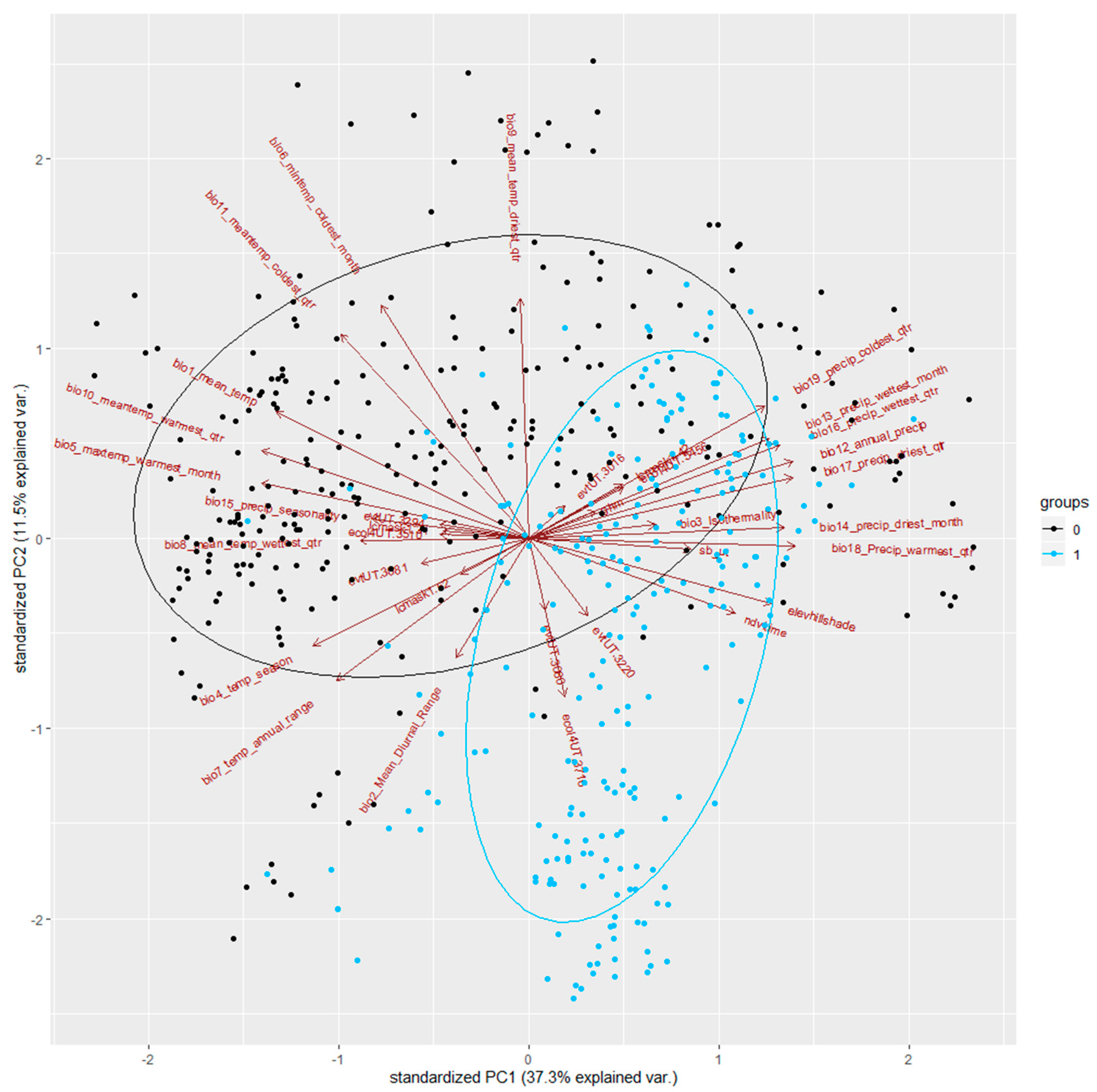
We extracted the predictors’ values where the wildlife data points were located and merged this list with the wildlife data frame, resulting in a final dataset, where we had values for each predictor for each observation and absence point (an example of a predictor can be seen in Figure 3).
In order to understand the importance of the different variables for the dataset, we performed a Principal Component Analysis (PCA), focused on gaining a better understanding of the structure of our data. We transformed the skewed predictors, and scaled and centered the data beforehand. We also needed to apply the one-hot encoding method, to create dummy variables for the categorical variables (land cover, ecoregions and Existing Vegetation (EVT)), followed by a preprocessing method in order to avoid a zero or near-zero value, which reduced the dataset to 34 variables.
In Figure 4, we can inspect the observations and pseudo-absences across the environmental space that PCA produces. To interpret the biplot, the rules are:
(1).
The X-axis represents PC1, the first component of the PCA, and the Y-axis represents the second component, PC2;
(2).
The points in blue are presence points, and those in black, absence points;
(3).
The ellipses represent the average distributions of the presence and absence points;
(4).
The arrows represent variables, and when two variables are pointing in the same direction or opposite directions, they are highly dependent (thus, independent when pointing in orthogonal directions);
(5).
The longer the arrow, the higher the importance of the variable for the overall environmental variation.
We can see that most of the presence points (in blue) occupy a specific space, defined by PC1 and PC2, where the variation is largely explained by PC2. It is also possible to identify some variables that are correlated with each other (collinearity). We can see that all the remaining ecoregion categories were positively correlated with most of the EVT categories, explaining the same variations. The same observation can be drawn for some of the temperature and precipitation layers, where some of the latter are negatively correlated with some of the former. The importance of the temperature variables is also visible, by the fact that some of the arrows representing these (such as Bio2_Mean_Diurnal_Range) follow the longest axes of the species’ ellipses (sage-grouse distribution).
At the same time, we also computed a correlation matrix, with all our environmental variables, so we could understand and detect collinearity between the variables. We used the corrplot function of the corrplot package [45], a package dedicated to the visualization of correlation matrices. The correlation matrix (Figure 5) shows the pairwise correlation between two variables, where the areas of the squares show the absolute value-corresponding correlation coefficients.
At first glance, it is easy to detect a strong correlation between the climatic variables, especially among the precipitation and temperature variables. It is also possible to detect some correlation of these climatic variables with elevation. The other variables have very little- or less-relevant values.
We calculated the Pearson correlation coefficients between all the 27 environmental variables and then proceeded to check both correlation and importance with a pairs plot function. We applied a threshold of 0.85 for the correlation coefficient, selecting those variables that had a higher correlation and excluding the ones that were of least importance for explaining the variation of our data. The layers that were finally excluded are the following: Bio2, Bio4, Bio5, Bio6, Bio10, Bio11, Bio15, Bio16, Bio17, Bio18, Bio19 and the ecoregions, with a remaining final total of 15 predictors.
We extracted the environmental data for each of the points in the dataset, obtaining a data frame with both the presence and background sage-grouse points, and we then split the data into training (70%) and testing (30%) data [46]. The split was made with a function that creates stratified random splits within each class, so that the distribution under each class is preserved as much as possible (function createDataPartition from caret package) [47]. To guarantee reproducibility, we set a seed number prior to the partition.
For RF, SVM and ANN model training, the caret package was utilized, while for MaxEnt, we used the dismo package. For all the models, we used the same partitioned data.

Setting up for RF, SVM and ANN Models

For this paper, supervised classification was used as the approach for ML algorithms, which can be automated for larger areas, a benefit when studying the statewide area of Utah, which covers 219,887 km2. Using ML algorithms, present sage-grouse sites were mapped, and thereafter, the probabilistic modeling of future sites could be predicted. The visualization of the maps resulting from the outputs can be accessed in the supplementary materials.
The classification algorithms used were deemed suitable for our study due to the absence of any assumption of normal distribution; their abilities to deal with the complexities of feature space, patterns and relationships; and the robustness of each model. Moreover, the choice of both categorical and continuous input allowed for flexibility in the predictor variables used.
To perform the training model, some parameters had to be included:
  • trainControl: defines the type and number of resampling, as well as the search method. We used cross-validation with 10 folds, and with random search.
  • metric: determines how the final model is defined, by selecting the tuning parameters with the highest value of the objective function. Amongst the functions available, we set it to “Accuracy”.
  • tuneLength: sets the size of the default grid of the tuning parameters; set to 15 for all our models.
  • preProcess: we selected to center and scale before resampling.
The parameters were selected according to the literature, as well as by exploring different possible combinations, and their effects on the performance of the model. For the RF model, it was necessary to define the number of trees, which was set to 1000. For reproducibility, we set a seed number before each model. After completing our training set up, we ran each model and studied their outputs. After their final tuning, we ran the predictions for each model based on the trained model and on the layer of stacked predictors. This produced a plotted output of a suitability map that presented the areas predicted as habitats and non-habitats in the study area. The process of setting up MaxEnt was slightly different: MaxEnt is included in the dismo package, and the presence/background vectors could not be used in the form of a factor, unlike for the other models, but categorical data had to be transformed into a factor.
Once the model was created, we generated a first prediction map, which gave a map with the probabilities of each pixel in the area being suitable/unsuitable, ranging from 0 to 1. This was performed with the raw output of the model and differed from the other algorithms in that the default output was not a binomial suitability map. To create the binomial map, it is necessary to apply a threshold to the prediction map. Then, we proceeded to evaluate the MaxEnt model with the test data by using the evaluate function from dismo. The evaluation required the test data (with the environmental data) to be separated into presence and absence. Therefore, the test data were split according to these two categories. Then, the evaluation was performed with the test data, and the MaxEnt model was created.
The output is an evaluation model file that includes all the parameters necessary to evaluate the model. Since the other algorithms’ prediction maps are binomial ones showing suitable/unsuitable habitats, it was necessary to apply the True Skill Statistic (TSS) threshold to the predicted probability map from MaxEnt to transform it into a binomial map that we could compare with the outputs from the other models. We based the evaluation of each model’s credibility on performance-based statistics: Cohen’s kappa, Omission and Commission errors, Accuracy, and the confusion matrices; all provide relevant and useful information in model analysis.
The Omission and Commission Error can be used to analyze the accuracy of the models when classifying the input points. The Omission Error refers to reference points that were left out (or omitted) from the correct class in the classified map, while the Commission Error refers to sites that are classified as reference points that were left out (or omitted) from the correct class in the classified map.
From these errors, it is also possible to calculate the User’s and Producer’s Accuracy. The Producer’s Accuracy is calculated as 1−Omission Error, and it translates into the percentage of reference points that were not omitted, whilst the User’s Accuracy is calculated as 1−Commission Error for each of the classes and accounts for the percentage of correctly classified sites or pixels. For further assessment of the models, an external evaluation was performed for the state of Idaho, addressed later on in the paper.

Future Predictions for Each Scenario

For the future predictions, we used only the environmental data that were available with future scenarios, namely, the climatic variables from WorldClim, Land Cover and Elevation. Other environmental layers used previously were not included, since the same variables were needed for current and future scenarios.
Once all the data were collected and preprocessed, we followed the same steps in building the models as we did before for the present data, following the same code. Once the models were created again, we loaded the future layers into R to prepare for the predictions. The future raster layers were read into R and stacked accordingly. We performed two predictions with each algorithm, one for each of the climate change scenarios selected (SSP2-4.5 and SSP3-7.0). Once run through future habitat prediction models for each of the algorithms, the outputs were saved in .tif and .grd formats, which could then be read into a GIS software for further visualization and post-processing. All the outputs can be visualized in the supplementary materials.

5. Results

5.1. Present

In all the models, we can see that the pseudo-absence class is the one with the most uncertainty, having a higher Omission Error and lower Producer’s Accuracy, and hence was not being classified as unsuitable habitats but mistakenly included into the suitable class (Table 5). On the other hand, all the models work better when classifying the presence class, omitting between 8 and 12% of the total of the actual presences, which are then included in the unsuitable habitat class.
Overall, looking at the Producer’s Accuracy, all the models seem to perform better when classifying the presences, which translates into fewer errors when predicting unsuitable habitats. The misclassified sage-grouse in unsuitable habitats range from 6 to 8%, the User’s Accuracy for the unsuitable habitat class being the highest for all the models. On the other hand, the lowest accuracy for all the models is exhibited by the User’s Accuracy for the suitable class, which means that the models do not perform as well when classifying the absences and thus wrongly include them into the suitable habitat class 15 to 24% of the time. The model with the lowest performance for this is SVM. This means that, when we look at the predictions made by these models, we can trust the unsuitable habitat prediction more because, although the models classify the presence points really well, they are less able to distinguish absence points and often misclassify them into suitable habitats. However, the User’s Accuracy for all the models is high, correctly predicting 75–84% of suitable habitats, meaning that they still perform well regardless of the errors.
After examining the models’ Confusion Matrices (CMs) and accuracies, it is possible to see that some models perform better than others. Based on the User’s and Producer’s Accuracy, the best performing model is the RF, closely followed by MaxEnt. These are also the best-performing models when looking at the overall accuracy of the models (Table 6).
Based on the kappa value interpretation by Landis and Koch [48], a kappa value between 0.61 and 0.80 indicates that there is substantial agreement, while 0.81–1.0 indicates perfect agreement. In our case, all the kappa values can then be considered good. In this case, the best classifier would be MaxEnt, being approximately 80% better than a random classification, being nearly in perfect agreement. The worst kappa value is the one obtained with the SVM model, although it still falls in the range where there is substantial agreement. However, this low kappa along with the lower accuracies indicates that this model did not perform as well with the current data and the tuning used for the models, thus providing the least accurate outcomes.
Overall, it seems that the RF and MaxEnt models are the most robust of them all under these circumstances (tuning and data), obtaining very high parameters, which implies that they are both accurate in the classification of these data.

External Validation

As a final test of the suitability of our model, it underwent an external validation to ascertain whether the model was making good predictions or was simply overfitted to the training data. In our case, the state of Idaho was selected because it also has a significant area of sage-grouse habitats and is adjacent to Utah, running north of the state’s border.
For our external validation, we used the same input variables as those used to create the model, clipped to the state of Idaho. We used the VGI sage-grouse observations for Idaho, also taken from the GBIF database. The idea of this external validation was that, if a habitat prediction for Idaho was made using the same input variables using the RF model, then, ideally, all or most of the VGI observations would be in areas our prediction designated as ”habitat”.
The classification rate indicates only a 65% success rate in confirming areas as habitats or non-habitats based on the VGI points (Table 7). Although these results are reasonable, they certainly leave room for improvement. Figure 1 shows both the current and historical ranges of the sage-grouse, and it is evident that there is agreement between our model’s results and the official distribution map.
Interestingly, there is a region in the south-west of Idaho (Figure 6) where a population of sage-grouse is observed in an area that our model designates as a non-habitat. This suggests shortcomings in our model, most likely due to inadequate tuning or a sub-optimal combination of input variables.

5.2. Future

From the predictions made with future environmental data, we obtained several maps representing the results from the different models and different climate change scenarios (Figure 7). The predictors chosen were those that had the highest variable importance as seen in Figure 8.
We can see that the sage-grouse habitat is reduced in all the future emission scenario models. Most of the habitat loss seems to occur in the center of the study area, leaving two relatively large disconnected areas of habitat in the north and south of the state, which are also patchier than in the current situation. Thus, all the models show that the habitats for sage-grouse will be greatly reduced in future scenarios, but also that landscape connectivity will be highly affected.

6. Discussion

6.1. Current Situation and Overall Performance of the Models

6.1.1. How Accurately Can Sage-Grouse’s Habitats Be Classified Using Each of the Selected Machine Learning Algorithms Based on Both Continuous and Categorical Variables?

Based on the results obtained from all the models, we can see that MaxEnt and RF seem to greatly outperform the other two models in terms of accuracy, which is further consolidated by the kappa. Within this section, however, we decided to focus on the results of the RF model. MaxEnt is a very robust model and one that is especially made for PO data. However, RF is equally robust and has more room for improvement in terms of model tuning and data. When, in the future, true absence data might be available, RF could be recommended over MaxEnt, as MaxEnt is not a presence–absence model [44]. Thus, we decided on RF, not only thinking about the current study but also potential improvements.
As seen in the results, the RF model performed best when classifying the presence points, showing a higher sensitivity. This, however, translates into a higher Omission Error for the absence points, which results in a more inaccurate prediction of the suitable class, as more absence points are misclassified into this class. This might be related to the creation of the pseudo-absences. We decided to create random pseudo-absences outside a presence area, generating a number that was close to the number of presences, as this was the best method for RF suggested by the literature reviewed. However, the User’s Accuracy for the suitable habitat was still high, as 83% of the predicted suitable habitat was, in fact, suitable, while only 17% of the predicted suitable habitat was incorrectly included in this class.
The inclusion of different types of environmental data proved to be beneficial for the overall prediction of the sage-grouse habitats in Utah. At the initial stage of building our models, a bigger focus on having different layers of temperature and precipitation led to satisfactory results concerning the performance of the models. However, it also showed a “thin” understanding of the variations of the habitat areas across the study area and of the ecological meaning of the variables for sage-grouse. Gathering a more comprehensive set of environmental data, based on the ecological aspects of the species whose habitats we are predicting [14,49,50,51], is best practice considering our modelling objective.
The downside of including environment layers with different levels and dimensions of measurements is reflected in the difficulty in making sure the data are preprocessed in order to fit the different models. Data transformation is part of some of the literature’s techniques to deal with variations in the levels of values in a dataset, so the important and necessary information is included in the model (also frequently expressed as “garbage in, garbage out”). Using supervised and unsupervised methods for this goal allowed us to identify the layers with the higher correlation and thus reduce multicollinearity. With the correlation threshold set to 0.85, we could identify that many of the temperature and precipitation layers demonstrated high correlation. According to Guisan et al. (2017) [51], there is no real consensus on an acceptable threshold to use, where much of the literature chooses to use r = 0.8 or r = 0.7. Therefore, we could reduce our variables into a final group that led to a compromise between having good model performance and reflecting an approximation of the true components of the species habitat.
The final dataset of environmental variables can be considered a fair representation of the characteristics of the habitats where sage-grouse are present. We know that sagebrush is greatly important and a main element of the sage-grouse diet, and that the weather conditions can affect the breeding period, besides the overall balance of the habitat. The sage-grouse is also found in areas with an elevation range of 4000 to 9000 feet (1200 to 2700 m, approximately) and prefers sagebrush landscapes [52]. Our final predictors provide a strong summary of these characteristics.
The different models were responsive to the input of both categorical and continuous layers in their prediction, where each model had a different set of important variables for their results. The RF model had, as the most important variables, the annual temperature, elevation and time-integrated Normalized Difference Vegetation Index (NDVI) (Figure 9). During the validation stage for the models, we took out each of these variables and ran the model again. We could see that, except for the elevation layer, the models would produce worse results as expected from previously stated species preferences. However, according to Guisan et al. (2017) [51], elevation can help in explaining variations in other variables at a finer scale in areas with less or little climate gradient and, in this case, help to narrow down areas where the main vegetation inherent to the sage-grouse habitat is present (sagebrush).
Besides the components that help to predict the species’ habitats, we can also observe the impact of variables in order to predict non-habitat areas: where it is less likely to observe sage-grouse. The global Human Modification (gHM) has a considerable effect on the RF model, showing that the human modification of the territory can help to identify areas where the sage-grouse is less likely to be present. This might also add meaning to the fact that the sage-grouse habitat in Utah is characterized as fragmented, which is one of the reasons that the many stressors that the gHM reflects (such as continued human development, agricultural land conversion or irrigated pastures) can have an influence on the non-habitat prediction.
In this way, it is possible to gain an overview of what type of variables can be important for prediction models for a species’ habitat suitability. We can firstly say that there is a mechanistic relationship between the predictors and the observation data of the species’ distribution, where the biological and ecological processes are the basis of the data used for the models [51]. Secondly, when choosing variables for SDMs, we also need to consider the scale of our study area, since that will affect the decision of whether we should include both direct and indirect variables. In our study, the inclusion of different types of variables is important for predicting the habitats of sage-grouse, although, to exactly understand what drives the spatial distribution of our species, we would need to narrow down to the more direct variables. Consequently, we would need to have a longer period of studying the species, and include their seasonal behavior and breeding conditions, among other ecological processes, to understand which type of data to add. For a further development of this work, this could involve the addition of more RS imagery. This would then be useful for studying the species at a larger scale than the state of Utah, where it would be relevant. In summary, the direct and indirect data we have included in our models are useful for predicting the distribution of the sage-grouse, at the scale of our study area. Our analysis leads to a developed understanding of important mechanistic variables and their direct impact on the distribution of our species (for example, temperature, elevation, NDVI or EVT) but also variables that have an impact in limiting the distribution (such as the gHM and land cover).

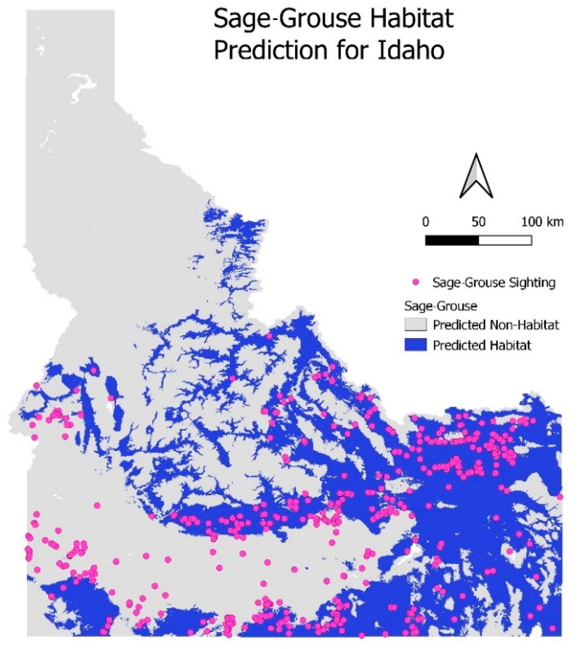
6.1.2. External Validation—Sage-Grouse Habitats in Idaho

The results here shed light on the feasibility of using ML techniques to make future predictions in general. While we achieved promising results with some of the models, the question is whether a model that is trained on present-day geographic data and volunteered sighting observations can be used with any confidence when considering future species distribution. The strongest indication we have of the suitability of our model for future use, or for areas other than Utah, are the results of the present-day species distribution prediction.
The results of the RF algorithm for the test data (Section 5 Results) indicate very good predictive power for the testing data. However, when conducting an external validation of the model with the same variables, paired with sage-grouse observations from the same VGI source, we see an immediate reduction in accuracy. Where the model in Utah achieved a correct classification rate of 89.7%, the same model used for prediction in Idaho predicted at only 65% accuracy.
There is a reduction in classification power when leaving the study area. The results achieved within the external validation suggest that there is room for improvement within the model. The immediate drop in predictive power once leaving the study area suggests that the model is overfitted to the data. An issue that could explain this is the inherent clustering of the data by species distribution. When dividing the data between training and testing, in most cases, the test data are taken from a cluster of either presences or absences. In this way, the algorithm has an easier job of classifying the testing points; if a testing point is removed from a cluster of “presence” training data, the likelihood that this point also is a “presence” point is very high. We saw this when experimenting with the number of pseudo-absence points that were used; when the number of pseudo-absences was increased, we saw a subsequent noticeable increase in the specificity of the model, as the areas these new points occupied already had classified areas of “absence”. However, this led to worse results for Sensitivity. This is to say that the model was very good at classifying absence points as more and more were included; however, the overall suitability of the model suffered. Future research could look at ways to remove this clustering problem by investigating alternative sources or formats for observation data.
As a side note, it is also important to remember that we are working with volunteered data that might contain some biases and inaccuracies, which could also negatively affect the results of the validation, for instance, unexpected presences outside the suitable habitats.

6.2. Future Predictions: Implications and Limitations

6.2.1. How Will the Sage-Grouse Habitats in Utah Be Impacted by the Varying Future Emission Scenarios That Represent the State’s Temperature Change Trajectory Most Closely?

As previously described, it has been estimated that air temperatures in Utah will rise by 1.67–2 °C within the next 30 years, with especially high temperatures during the summer [20], disturbing seasonal patterns, increasing drought and negatively impacting the present vegetation and, subsequently, all the wildlife in the state (i.e., [6,53]).
These predictions seem to be in line with our results. As seen in the maps obtained from the different ML algorithms, sage-grouse habitats will be negatively impacted by the changes in environmental factors caused by the temperature rise.
This loss of habitat is considerable from the present conditions, especially when looking at the SSP3-7.0 scenario. In this specific case, when comparing the original habitat prediction to the one obtained with this climate scenario, we see that the reduction in suitable habitat for the sage-grouse goes up to 69% (Figure 9).
For the SSP2-4.5 scenario, the loss of habitat is approximately 60%, which is still considerable since it means that, even in a more optimistic scenario, approximately two thirds of the current sage-grouse habitat will be lost within the next 30–40 years.
Moreover, the prediction maps obtained for both future climate scenarios seem to be in line with current predictions made specifically for sage-grouse habitats, in which they estimate that the species range will decrease by 71% for their breeding range and up to 92% for their winter range by 2080 [54]. Our predictions were made for the time period between 2041 and 2060, but since the temperature rise is expected to continue up to 2100, we can only expect that this trend will continue, and sage-grouse habitats will be further reduced.
Additionally, these predictions emphasize not only the loss of habitat but also the increase in habitat fragmentation, resulting in, as a result, a habitat composed of several small, unconnected patches. The sage-grouse is a very specialist species, having great difficulties in adapting to habitat change [55]. Going out of its habitat and through the inhospitable matrix to move from one patch to another is unlikely, and it would increase its mortality rate [56]. The edge effect, diverse physical and biotic alterations associated with the boundaries of the habitat fragment [57], will be more acute in these small patches, which might even be too small for the species to live in. Ultimately, the fragmentation could cause the isolation of some subpopulations of the species, which would likely become extinct due to problems such as inbreeding, diseases or bottleneck effects [58]. Since this species has very important seasonal movements [55], the fragmentation could greatly impact it by impeding its movement from its wintering areas to the breeding ones.
Of course, it is necessary to point out that, even though layers such as NDVI and sagebrush presence are important for sage-grouse and thus could have some effect on the predictions, they could not be added into the future predictions, as no estimates for the coming years were available. However, a land cover estimate was used (Section 3.3.2 Land Cover Future Scenarios), which shows how all different land uses, including vegetation and sagebrush, will change over time. Nevertheless, the land cover estimates already show that most vegetation, including bushy habitats, will decrease, and the effects of climate change will induce droughts and wildfires, negatively impacting vegetation [6]. This means that the predicted maps would probably not be too different from how they are now, even if NDVI and sagebrush estimates were available, as vegetation cover is expected to decrease, and loss of vegetation is ultimately linked to habitat loss for sage-grouse.

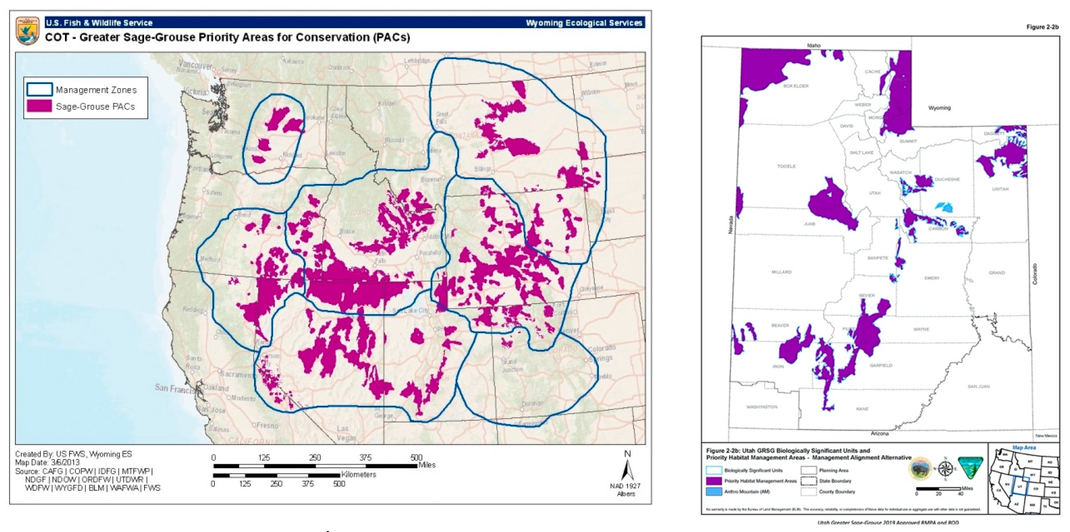
6.2.2. Based on the Prediction Maps for Future Scenarios Obtained from the Models, How Will the Change in Sage-Grouse Habitats Affect Current Conservation Areas?

Comparing the future prediction model outputs to already existing sage-grouse management plan maps further stresses the significance of negative impacts on biodiversity. The 2013 USFWS Greater Sage-grouse Conservation Objectives Final Report [59] established Priority Areas of Conservation (PACs) for sage-grouse habitats. These were areas defined as long-term key habitats for sage-grouse as well as areas for the potential restoration and maintenance of sagebrush shrub [59]. Statewide areas of conservation value were acknowledged as imperative for maintaining and representing resilient sage-grouse populations by way of lek counts, telemetry, the collection of observation data, nesting area identification and assessing previously known species distributions. According to the documentation, the FWS PACs aligned well with BLM’s preliminary priority sage-grouse habitat maps (Figure 10).
Despite being significantly reduced in total area, future models align similarly in the direction and placement of the USFWS and BLM PAC areas. However, the top performing model, RF, demonstrates a larger reduction of the conservation area in existing southern and central Utah sage-grouse habitats. In addition, RF exposes areas that could prove to be of critical importance for the future safeguarding of this species that have not been considered high value in these organizations’ planning efforts.
When analyzing the models under future emission scenario SSP2-4.5, a substantial area of the north-eastern corner can be seen to represent potential future habitats for sage-grouse that, again, has not been identified by either FWS or BLM as priority land. The variances are unsurprising due to a statement made in the FWS report indicating that the uncertainty of PACs cannot be reduced when considering the effects of climate change, as no climatic variables were used in their mapping process. Additionally, it appears that uncertainties surrounding energy development, sage-grouse population connectivity, demographic factors and vegetative health-related concerns are all flagged as reasons that conservation assessments based on these maps must remain flexible.
The RF future outputs from this study produced one of the more highly fragmented distributions of future sage-grouse habitats in comparison with the FWS and BLM maps. Some of these smaller, fractured, future-predicted parcels that were deemed suitable by the algorithm were insufficiently sized for inclusion after the post-processing of the future model output data. The reason for their removal, in addition to audience interpretability, was the average sage-grouse nest-to-lek distance.
Ultimately, RF shows that future changes in sage-grouse habitats renders some current PACs impractical and calls for additional areas to be considered for protection under conservation easement. Attention should be focused on maintaining connectivity between the habitats as much as possible between the south and northern habitat patches to avoid isolation between subpopulations of sage-grouse inhabiting these habitat patches. Although sage-grouse can travel through inhospitable habitats to get from one patch to another, this still increases their mortality, as previously discussed. Moreover, failure in maintaining connectivity could result in the complete isolation of some subpopulations of sage-grouse if their habitat is further reduced and the distances between patches increase. Maintaining connectivity will allow sage-grouse to easily migrate from small patches that are at risk of disappearing to bigger habitat patches that could support them, thus reducing the risk of extinction of the local subpopulations in the area. Additionally, it is important that sage-grouse can move not only within the state but also to other states to maintain the genetic diversity of the population, ensuring overall health and fitness [60].

How Do These Suggestions Follow the UN’s SDGs and the CBD Goals?

These suggestions directly incorporate the biosphere facet of the United Nations (UN) Sustainable Development Goals (SDGs) and could lead to further indirect impacts on both society and the economy as a result of progress in conservation assessment. Although suggesting deviations from current conservation framework construction could be met with resistance towards ML technology due to a lack of time or monetary resources for equipment, learning and implementation, the benefits seem to far outweigh the costs. Because this study used ML algorithms to measure the effect of climate change on the distribution of sage-grouse habitats, it conforms to the UN SDG mission slogan “If you can’t measure it, you can’t manage it.”. These future model outputs offer an opportunity to reassess current conservation strategies and potentially play other roles in following the UN SDGs [3] by the ways in which they can be put into practice for other future uses.
It is under the Goals 13 and 15 that this work directly approaches the UN SDGs. The future impacts of climate change could result in (and are already resulting in) dire outcomes for the entire biosphere of the planet, and it is necessary to integrate climate change measures into the responsible authorities’ strategies and planning (Target 13.2). The conservation authorities responsible for the management of protected areas should be urged to incorporate climate change-related measures not only to mitigate the fragmentation of sage-grouse habitats but also to prevent the further aggravation of the habitat deterioration, by taking a stance of identifying and protecting climate refugia, in order to cope with climate-driven changes [12]. It is an achievable and possible approach, to focus on vulnerability assessment and management for change (instead of static conditions), to be adopted in the overall mitigation, adaptation, impact reduction and early-warning for climate change (Target 13.3).
The protection of sage-grouse habitats will also have other positive restoration effects on the land, as we are dealing with a semi-arid region at risk of increasing land fires, drought and floods. By conserving and restoring bushy vegetation, the responsible authorities will also combat desertification and halt land degradation, striving to achieve a land degradation-neutral world (Target 15.3). Of course, the protection of sage-grouse habitats would also stop the obvious degradation of natural habitat and halt the loss of biodiversity, preventing the extinction of threatened species (Target 15.5).
Moreover, taking the measures discussed to protect not only sage-grouse habitats per se but also landscape connectivity to maintain their genetic diversity and overall population fitness will closely follow the main CBD goals.
With our current results, we can see that the future for sage-grouse and their habitats is uncertain, with a high risk of them disappearing. Moreover, this will not only mean the extinction of sage-grouse populations, but many other plant and animal species will also be affected by these changes in the ecosystem, decreasing the overall biological diversity in the area. Taking measures to protect this habitat will be key for many species apart from sage-grouse and will help in maintaining the current biodiversity in Utah, following the goals of the CBD and the UN SDGs.

7. Limitations

An obvious limitation of our model was that the raster climate variables used were assembled from data collected in 2010, while the VGI sage-grouse data were collected during the time period of 2000–2020. Ideally, our sage-grouse observations would be taken during the same time period as that during which our climate variables were produced. With the rapid changes caused by climate change, we introduce the possibility that sage-grouse habitats have already begun to change and that, particularly with older observations, sage-grouse have been observed in areas that no longer would be classified as its habitat. Thus, the results might change slightly when using more recent data, if they become available.
Moreover, and as discussed in the previous section, not all environmental layers have future estimations that can be used for future predictions, and they could be a useful addition for predicting changes in the sage-grouse habitats should they become available.
Additionally, we used volunteered PO data. As explained before, volunteered data can contain errors and biases. As we lacked the time and resources to obtain a better dataset, we decided to use them, since they were reliable enough for the purpose of this work. However, a higher-quality, unbiased, non-clustered dataset could bring improvements to the results obtained from the models, which could be seen with the drop in predictive accuracy on the external validation in Idaho. Similarly, the dataset would also improve if the pseudo-absences could be validated to some extent.

8. Conclusions

Ecosystem degradation and biodiversity loss is a reality that is already underway and advancing at a rapid pace, at risk of further aggravation from climate change. The goals outlined by the United Nations are set in order to avoid exceeding climate system tipping points, which can be aided by innovative techniques and tools, such as SDMs. For this study, we intended to analyze this problem by building a prediction model with a focus on the sage-grouse as a species, using ML algorithms, in addition to studying the impacts of climate change on the species’ habitat in Utah.
Using algorithms of different classes (maximum entropy, machine learning, and regression trees), which are also based on different conceptual approaches and statistical methods, is a useful approach to capturing the different relationships between the observation data and the predictor variables. Considering the analysis performed on the different models used, we can conclude that MaxEnt, with an accuracy of 0.897, is a very solid model, but RF—with an accuracy of 0.897 and a sensitivity and specificity of 0.917 and 0.885, respectively—seems to perform equally as well and has more room for improvement.
Although the future predictions of sage-grouse habitats for the state of Utah are limited, due to the lack of some environmental data, the predictions obtained for the different scenarios of temperature rise seem to align with current literature, with the loss of up to 70% of sage-grouse habitat. More work can be performed in this area with different datasets to improve the accuracy of the predictions.
We can also conclude that conservation efforts should be directed to mitigating the fragmentation of the sage-grouse habitat in Utah. The predictions produced in this study show that future changes in the species’ territory are not exactly in line with current PACs, calling for additional areas to be considered for protection under conservation easement. We point out that the emphasis of additional efforts should be placed on maintaining connectivity between the habitats in certain areas of the state, in order to avoid isolation between the subpopulations of sage-grouse present in these areas.
All in all, ML can play a crucial role in contributing to the UN SDGs, including the use of Earth Observation in the environmental dataset. SDMs coupled with ML can provide a better overview of the distributions of species and their habitats, current and future, and create awareness for conservation planning and decision-making as well as for demanding accountability.

9. Future Extension

A possible future extension of the paper’s findings includes the implementation of a Spatial Decision Support System (SDSS), the purpose of which would be to give stakeholders direct access to SDMs via Web GIS. This would enable the selection of species, variables and study areas for generating a distribution prediction, present or future. An additional extension would be to incorporate ensemble modeling. An ensemble model would take several input models—for example, RF, MaxEnt, SVM and ANN, which were used in this study—and would generate a model that is a combination of these input models, the rationale being that the result would be more adaptable. Finally, the development of PCA for prediction could further improve the performance of the algorithms by including the PCs in the models directly. This would require the further investigation of PCA/Non-Linear PCA techniques and their combination with prediction models.

Supplementary Materials

The following are available online at https://www.mdpi.com/2071-1050/12/18/7657/s1. The scripts created for and maps produced throughout this study are available as supplementary materials.

Author Contributions

Conceptualization, A.C.M.F., R.Q.G., M.A.L.-C., E.F.L.T. and J.J.A.; supervision, J.J.A.; writing—original draft, A.C.M.F., R.Q.G., M.A.L.-C. and E.F.L.T.; writing—review and editing, A.C.M.F., R.Q.G., M.A.L.-C., E.F.L.T. and J.J.A. All authors have read and agreed to the published version of the manuscript.

Funding

This research received no external funding.

Conflicts of Interest

The authors declare no conflict of interest.

References

  1. European Commission. 4 August 2009. Available online: https://ec.europa.eu/environment/nature/info/pubs/docs/climate_change/en.pdf (accessed on 25 May 2020).
  2. Convention on Biological Diversity. “Introduction,” Convention on Biological Diversity. 2012. Available online: https://www.cbd.int/intro/ (accessed on 31 May 2020).
  3. United Nations. About the Sustainable Development Goals. 2020. Available online: https://www.un.org/sustainabledevelopment/sustainable-development-goals/ (accessed on 31 May 2020).
  4. Zhang, J.; Li, S. A Review of Machine Learning Based Species’ Distribution Modelling. In Proceedings of the 2017 International Conference on Industrial Informatics—Computing Technology, Intelligent Technology, Industrial Information Integration, Wuhan, China, 2–3 December 2017. [Google Scholar]
  5. Burnett, C. Modeling Habitat Use of a Fringe Greater SageGrouse Population at Multiple Spatial Scales. Utah State University. July 2013. Available online: https://extension.usu.edu/wildlife-interactions/ou-files/faqs/Modeling-Habitat-Use-of-a-Fringe-Greater-Sage-Grouse-Population.pdf (accessed on 23 May 2020).
  6. United States Environmental Protection Agency. What Climate Change Means for Utah. August 2016. Available online: https://19january2017snapshot.epa.gov/sites/production/files/2016-09/documents/climate-change-ut.pdf (accessed on 20 May 2020).
  7. Bureau of Land Management. State Threatened and Endangered Information. Bureau of Land Managment. 2019. Available online: https://www.blm.gov/programs/fish-and-wildlife/threatened-and-endangered/state-te-data/utah (accessed on 23 May 2020).
  8. Climate Central. Utah. 2020. Available online: https://statesatrisk.org/utah/all (accessed on 31 May 2020).
  9. Wilson, M.C.; Chen, X.Y.; Corlett, R.T.; Didham, R.K.; Ding, P.; Holt, R.D.; Holyoak, M.; Hu, G.; Hughes, A.C.; Jiang, L.; et al. Habitat fragmentation and biodiversity conservation: Key findings and future challenges. Lands. Ecol. 2016, 31, 219–227. [Google Scholar] [CrossRef] [Green Version]
  10. Crooks, K.R.; Burdett, C.L.; Theobald, D.M.; King, S.R.; di Marco, M.; Rondinini, C.; Boitani, L. Quantification of habitat fragmentation reveals extinction risk in terrestrial mammals. Proc. Natl. Acad. Sci. USA 2017, 114, 7635–7640. [Google Scholar] [CrossRef] [PubMed] [Green Version]
  11. Huettmann, F. Machine Learning for ‘Strategic Conservation and Planning’: Patterns, Applications, Thoughts and Urgently Needed Global Progress for Sustainability. In Machine Learning for Ecology and Sustainable Natural Resource Management; Springer: Berlin, Germany, 2018. [Google Scholar]
  12. Game, E.T.; Lipsett-Moore, G.; Saxon, E.; Peterson, N.; Sheppard, S. Incorporating climate change adaptation into national conservation assessments. Glob. Chang. Biol. 2011, 17, 3150–3160. [Google Scholar] [CrossRef]
  13. Oliver, T.H.; Smithers, R.J.; Bailey, S.; Walkmsley, C.A.; Watts, K. A decision framework for considering climate change adaption in biodiversity conservation planning. J. Appl. Ecol. 2012, 49, 1247–1255. [Google Scholar] [CrossRef]
  14. Baltensperger, P.; Huettmann, F. Predictive spatial niche and biodiversity hotspot models for small mammal communities in Alaska: Applying machine-learning to conservation planning. Lands. Ecol. 2015, 30, 681–697. [Google Scholar] [CrossRef]
  15. Shaw, R. The 10 Best Machine Learning Algorithms for Data Science Beginners. Dataquest Labs, Inc. 2019. Available online: https://www.dataquest.io/blog/top-10-machine-learning-algorithms-for-beginners/ (accessed on 31 May 2020).
  16. Elith, J.; Leathwick, J.R. Species Distribution Models: Ecological Explanation and Prediction across Space and Time. Annu. Rev. Ecol. Evol. Syst. 2009, 40, 677–697. [Google Scholar] [CrossRef]
  17. Aguirre-Gutiérrez, J.; Raes, N. A Modeling Framework to Estimate and Project Species Distributions in Space and Time. Mt. Clim. Biodivers. 2018, 309–320. [Google Scholar]
  18. Sofaer, H.R.; Jarnevich, C.S.; Pearse, I.S.; Smyth, R.L.; Auer, S.; Cook, G.L.; Edwards, T.C., Jr.; Guala, G.F.; Howard, T.G.; Morisette, J.T.; et al. Development and Delivery of Species Distribution Models to Inform Decision-Making. BioScience 2019, 69, 544–557. [Google Scholar] [CrossRef]
  19. Netstate. Utah: The Geography of Utah. NSTATE, LLC. 25 February 2016. Available online: https://www.netstate.com/states/geography/ut_geography.htm (accessed on 26 May 2020).
  20. Utah Rivers Council. Climate Change. 2020. Available online: https://utahrivers.org/climate-change (accessed on 28 May 2020).
  21. NatureServe. Utah Conservation Summary. 2020. Available online: http://www.landscope.org/utah/overview/ (accessed on 29 May 2020).
  22. Park City Municipal. Community & Municipal Carbon Footprint. 2020. Available online: https://www.parkcity.org/departments/sustainability/community-municipal-carbon-footprint (accessed on 4 May 2020).
  23. USFWS. Greater Sage-grouse Conservation in Utah. U.S. Fish & Wildlife Service. 2020. Available online: https://www.fws.gov/greatersagegrouse/factsheets/UTGrSGFactSheet_FINAL.pdf (accessed on 15 May 2020).
  24. Opar, Tick Tock Goes the Sage-Grouse Conservation Clock; National Audobon Society: October 2015. Available online: https://www.audubon.org/magazine/september-october-2015/tick-tock-goes-sage-grouse (accessed on 16 May 2020).
  25. Connelly, J.W.; Knick, S.T.; Schroeder, M.A.; Stiver, S.J. Conservation Assessment of Greater Sage-Grouse and Sagebrush Habitats. DigitalCommons@USU; Western Association of Fish and Wildlife Agencies: Cheyenne, WY, USA, 2004. [Google Scholar]
  26. Stauffer, M.; Curtis, L.D. Governor: Utah Will Implement New Controversial Plan for Sage Grouse. KUTV. 15 January 2019. Available online: https://kutv.com/news/local/governor-utah-will-implement-new-plan-to-conserve-sage-grouse (accessed on 15 May 2020).
  27. Utah DNR. Greater Sage-Grouse. State of Utah. 1 May 2019. Available online: https://wildlife.utah.gov/greater-sage-grouse.html (accessed on 15 May 2020).
  28. Institute for Applied Ecology. Five Things You Didn’t Know About Sagebrush. 2020. Available online: https://appliedeco.org/five-things-you-didnt-know-about-sagebrush/ (accessed on 20 May 2020).
  29. Strategic Management Plan for Sage-grouse; Utah Division of Wildlife Resources: Salt Lake City, Utah, 2002.
  30. The National Wildlife Federation. Greater Sage-Grouse. The National Wildlife Federation. 2020. Available online: https://www.nwf.org/Educational-Resources/Wildlife-Guide/Birds/Greater-Sage-Grouse (accessed on 5 May 2020).
  31. Global Biodiversity Information Facility. 2020. Available online: https://www.gbif.org/ (accessed on 23 May 2020).
  32. Aarts, G.; Fieberg, J.; Matthiopoulos, J. Comparative interpretation of count, presence–absence and point methods for species distribution models. Methods Ecol. Evol. 2012, 3, 177–187. [Google Scholar] [CrossRef]
  33. Phillips, S.J.; Dudik, M.; Elith, J.; Graham, C.H.; Lehmann, A.; Leathwick, J.; Ferrier, S. Sample Selection Bias and Presence-Only Distribution Models: Implications for Background and Pseudo-Absence Data. Ecol. Appl. 2009, 19, 181–197. [Google Scholar]
  34. Senay, S.D.; Worner, S.P.; Ikeda, T. Novel Three-Step Pseudo-Absence Selection Technique for Improved Species Distribution Modelling. PLoS ONE 2013, 8, e71218. [Google Scholar]
  35. Dahlgren, D.K.; Messmer, T.; Crabb, B.A.; Larsen, R.T. Seasonal Movements of Greater Sage-grouse Populations in Utah: Implications for Species Conservation. Wildl. Soc. Bull. 2016, 40, 288–299. [Google Scholar] [CrossRef]
  36. Barbet-Massin, M.; Jiguet, F.; Albert, C.H.; Thuiller, W. Selecting pseudo-absences for species distribution models: How, where and how many? Methods Ecol. Evol. 2012, 3, 327–338. [Google Scholar]
  37. WorldClim. Downscaling Future and Past Climate Data from GCMs; WorldClim. 2020. Available online: https://worldclim.org/data/downscaling.html (accessed on 14 May 2020).
  38. Sohl, T.; Sayler, K.; Bouchard, M.; Reker, R.; Freisz, A.; Bennett, S.; Sleeter, B.; Sleeter, R.; Wilson, T.; Soulard, C.; et al. Conterminous United States Land Cover Projections—1992 to 2100, ScienceBase-Catalog. 2017. Available online: https://www.sciencebase.gov/catalog/item/5b96c2f9e4b0702d0e826f6d (accessed on 24 May 2020).
  39. Scikit-learn. Scikit-learn: Machine learning in Python. Scikit-learn. 2020. Available online: https://scikit-learn.org/stable/ (accessed on 25 August 2020).
  40. Gautier, L. rpy2 3.3.5. pypi.org. 2020. Available online: https://pypi.org/project/rpy2/ (accessed on 25 August 2020).
  41. Maxwell; Warner, T.; Fang, F. Implementation of machine-learning classification in remote sensing: An applied review. Int. J. Remote Sens. 2018, 39, 2784–2817. [Google Scholar]
  42. Zhou, V. Machine Learning for Beginners: An Introduction to Neural Networks. Towards Data Science. 2019. Available online: https://towardsdatascience.com/machine-learning-for-beginners-an-introductionto-neural-networks-d49f22d238f9 (accessed on 27 May 2020).
  43. Merow, C.; Smith, M.J.; Silander, J.A., Jr. A practical guide to MaxEnt for modeling species’ distribution: What it does, and why inputs and settings matter. Ecography 2013, 36, 1058–1069. [Google Scholar]
  44. Guillera-Arroita, G.; Lahoz-Monfort, J.J.; Elith, J. Maxent is not a presence–absence method: A comment on Thibaud et al. Methods Ecol. Evol. 2014, 5, 1192–1197. [Google Scholar]
  45. Wei, T.; Simko, V. Package ‘corrplot’. 17 October 2017. Available online: https://cran.r-project.org/web/packages/corrplot/corrplot.pdf (accessed on 31 May 2020).
  46. Bungaro, L. How to Evaluate your Machine Learning Model. Medium. 31 July 2018. Available online: https://medium.com/coinmonks/debugging-a-learning-algorithm-ef7c16936864 (accessed on 25 May 2020).
  47. Kuhn, M. Caret Package. J. Stat. Softw. 2008, 28, 1–26. [Google Scholar]
  48. Landis, J.R.; Koch, G.G. An Application of Hierarchical Kappa-type Statistics in the Assessment of Majority Agreement among Multiple Observers. Biometrics 1977, 33, 363–374. [Google Scholar] [CrossRef]
  49. Duan, R.-Y.; Kong, X.-Q.; Huang, M.-Y.; Fan, W.-Y.; Wang, Z.-G. The Predictive Performance and Stability of Six Species Distribution Models. PLoS ONE 2014, 9, e112764. [Google Scholar] [CrossRef] [Green Version]
  50. Elith, J.; Graham, C.H.; Anderson, R.P.; Dudı´k, M.; Ferrier, S.; Guisan, A.; Hijmans, R.J.; Huettmann, F.; Leathwick, J.R.; Lehmann, A.; et al. Novel methods improve prediction of species’ distributions from occurrence data. Ecography 2006, 29, 129–151. [Google Scholar] [CrossRef] [Green Version]
  51. Guisan, A.; Thuiller, W.; Zimmermann, N.E. Habitat Suitability and Distribution Models: With Application in R, Vols. Ecology, Biodiversity and Conservation; Cambridge University Press: Cambridge, UK, 2017. [Google Scholar]
  52. Rowland, M.M.; Vojta, C.D. A Technical Guide for Monitoring Wildlife Habitat; Forest Service: Washington, DC, USA, 2013. [Google Scholar]
  53. Shultz, L. Pocket Guide to Sagebrush. 2012. Available online: http://www.sagegrouseinitiative.com/wp-content/uploads/2013/07/SGI_Sagebrush_PocketGuide_Nov12.pdf (accessed on 20 May 2020).
  54. National Audubon Society. Greater Sage-Grouse. 2019. Available online: https://climate2014.audubon.org/birds/saggro/greater-sage-grouse (accessed on 21 May 2020).
  55. Connelly, J.W.; Rinkes, E.T.; Braun, C.E. Chapter Four Characteristics of Greater Sage-Grouse Habitats: A Landscape Species at Micro-And Macroscales. In Greater Sage-Grouse: Ecology and Conservation of a Landscape Species and Its Habitats; University of California Press: Berkeley, CA, USA, 2011. [Google Scholar]
  56. Knick, S.T.; Connelly, J.W. Greater Sage-Grouse: Ecology and Conservation of a Landscape Species and Its Habitats; University of California Press: Berkeley, CA, USA, 2011; p. 664. [Google Scholar]
  57. Laurance, W.F.; Nascimento, H.E.M.; Laurance, S.G.; Andrade, A.; Ewers, R.M.; Harms, K.E.; Luizão, R.C.C.; Ribeiro, J.E. Habitat Fragmentation, Variable Edge Effects, and the Landscape-Divergence Hypothesis. PLoS ONE 2007, 2, e1017. [Google Scholar] [CrossRef] [PubMed]
  58. Davis, D.M.; Reese, K.P.; Gardner, S.C.; Bird, K.L. Genetic structure of Greater Sage-Grouse (Centrocercus urophasianus) in a declining, peripheral population. Condor 2015, 117, 530–544. [Google Scholar]
  59. U.S. Fish and Wildlife Service. Greater Sage-grouse (Centrocercus urophasianus) Conservation Objectives: Final Report. February 2013. Available online: https://www.fws.gov/greatersagegrouse/documents/COT-Report-with-Dear-Interested-Reader-Letter.pdf (accessed on 31 May 2020).
  60. Vrijenhoek, R.C. Genetic Diversity and Fitness in Small Populations. In Conservation Genetics; Birkhäuser: Basel, Switzerland, 1994; pp. 37–53. [Google Scholar]
Figure 1. Map showing the current and historic range of sage-grouse in the US (US Fish and Wildlife Service (USFWS), 2020).
Sustainability 12 07657 g001
Figure 2. Sage-grouse observations.
Sustainability 12 07657 g002
Figure 3. Example of a predictor plot (Bio1—Mean Temperature).
Sustainability 12 07657 g003
Figure 4. Biplot of PC1 and PC2 for all transformed data.
Sustainability 12 07657 g004
Figure 5. Correlation Matrix of all variables.
Sustainability 12 07657 g005
Figure 6. External validation: current habitat prediction for sage-grouse in Idaho using selected model.
Sustainability 12 07657 g006
Figure 7. Comparison between the model’s predictions for present conditions (left) and future predicted scenarios (right).
Sustainability 12 07657 g007
Figure 8. Plot and output expressing the general effects of the predictors on the model.
Sustainability 12 07657 g008
Figure 9. RF model predictions for current and future sage-grouse habitats.
Sustainability 12 07657 g009
Figure 10. USFWS (left) and Bureau of Land Management (BLM) (right) identified areas of importance for sage-grouse (USFWS 2014, BLM 2019).
Sustainability 12 07657 g010
Table 1. Comparative summary of previous research on Machine Learning (ML) in Species Distribution Models (SDMs).
MethodologyUseStrengthsWeaknessesSource
Use of Remote Sensing imagery to calculate vegetation extent, several environmental layers as background data and museum observations for species data. The MARXAN software was used for all planning strategies and run multiple times with target set dataConservation strategy, implementation and assessment in response to biodiversity loss in Papua New GuineaAddresses the static, unproductive approach to current conservation assessment efforts in this location, addresses impact of climate change on species relocation. Discovery that geophysical data should be used in conjunction with environmental layers for reliability of resultsTheoretically based research, more concentrated on current conservation assessment procedures and limited in terms of tools used[12]
Machine Learning algorithm Decision Trees is used to determine current and future species distribution Creation of a decision framework enabling the identification and prioritization of current conservation-related actionEnables an adaptive strategy plan, inclusive of science, policy and practice. Can be used for local management for species at risk on a universal level. Combines both theoretical and practical knowledge of conservation, where restricted information can inhibit rational planningRequires expert insight when determining answers for each of the three potential Decision Tree algorithm outputs regarding species adaptability; Adversely Sensitive, Climate Overlap, and New Climate Space[13]
Use of both archived and openly accessible records for presence data of species, confirmed by ground truthing methods. Random Forest Machine Learning algorithm, in addition to TreeNet, Mars, CART and MaxEnt, in combination with top-performing predictor variables, assessed future conservation areas for investigated species Establish present distribution and territory of small mammals at northern latitudes whilst considering forced relocation as a consequence of habitat alteration due to climate changeConcludes points for successful methodology and provides an initial framework for species mapping and monitoring that can be implemented on a broader spatial–temporal scale. Provides advanced material for Machine Learning algorithms used in species distribution modeling. Offers insight into understanding predictor variables and resolutions [14]
Machine Learning algorithm MaxEnt is used alongside Very High Frequency telemetry technology and predictor variables in locating undiscovered seasonal distributions of sage-grouseDetermine and model habitat preferences of periphery populations of sage-grouse Considers both environmental and anthropogenic variables. All four final models produced demonstrated excellent predictability upon visual inspection. Contributes to the further understanding of Machine Learning algorithms, Species Distribution Models and individual characteristics of sage-grouse speciesCertain areas highlighted by results indicated necessary further investigation in order to determine species distribution[5]
Table 2. Data variables and sources for current data. (* The data shaded in gray were not included in the final dataset.).
NameSub-CategoryTypeResolutionYearSource
Bioclimatic VariablesBIO1 Annual Mean TemperatureContinuous1 km1970–2000worldclim.org
* BIO2 Mean Diurnal Range (Mean of monthly (max temp-min temp))
BIO3 Isothermality (BIO2/BIO7) (x100)
* BIO4 Temperature Seasonality (standard deviation x100)
BIO5 Max Temperature of Warmest Month
BIO6 Min Temperature of Coldest Month *
BIO7 Temperature Annual Range (BIO5–BIO6)
BIO8 Mean Temperature of Wettest Quarter
BIO9 Mean Temperature of Driest Quarter
* BIO10 Mean Temperature of Warmest Quarter
* BIO11 Meant Temperature of Coldest Quarter
BIO12 Annual Precipitation
BIO13 Precipitation of Wettest Month
BIO14 Precipitation of Driest Month
BIO15 Precipitation Seasonality (Coefficient of Variation)
* BIO16 Precipitation of Wettest Quarter
* BIO17 Precipitation of Driest Quarter
* BIO18 Precipitation of Warmest Quarter
* BIO19 Precipitation of Coldest Quarter
* EcoregionsLevel IVCategoricalN/A (.shp)2012United States Environmental Protection Agency
ElevationAuto-correlated DEMContinuous2 m2018Utah AGRC
Global Human Modification (gHM) Continuous1 km2016Conservation Science Partners, GEE
Multi-Resolution Land CharacteristicsCONUS Urban ImperviousnessContinuous30 m2016MRLC Consortium
CONUS Land CoverCategorical 2016
CONUS Sagebrush Shrubland Fractional ComponentContinuous 2016
Existing Vegetation (EVT) Categorical30 m2014LANDFIRE
Normalized Difference Vegetation Index (NDVI)Time integratedContiguous1 km2013USGS Earth Explorer
Table 3. Data variables and sources for future data.
NameSub-CategoryTypeResolutionYearSource
Bioclimatic VariablesBIO1 Annual Mean TemperatureContinuous4.5 km2041–2060worldclim.org
BIO3 Isothermality (BIO2/BIO7) (x100)
BIO7 Temperature Annual Range (BIO5–BIO6)
BIO8 Mean Temperature of Wettest Quarter
BIO9 Mean Temperature of Driest Quarter
BIO12 Annual Precipitation
BIO13 Precipitation of Wettest Month
BIO14 Precipitation of Driest Month
BIO15 Precipitation Seasonality (Coefficient of Variation)
ElevationAuto-correlated DEMContinuous2 m2018Utah AGRC
Multi-Resolution Land CharacteristicsCONUS Land CoverCategorical250 m2100MRLC Consortium
Table 4. Summary of hyperparameters for each model algorithm.
ModelHyperparameters
Support Vector Machines (RBF)Sigma: determines the reach of a single training instance
Random forestsC (cost): controls training errors and margins
Artificial Neural NetworksMtry: number of variables randomly sampled as candidates at each split
Table 5. Result table of the Confusion Matrix, Omission and Commission Errors, and Producer and User Accuracies for all the models.
01 Omission ErrorCommission ErrorProducer AccuracyUser Accuracy
0797860.1770.08140.8230.919SVM
11753700.1170.2430.8830.757
9660156
0828900.1460.0890.8540.911ANN
11452660.1330.2120.8670.788
9660156
0855900.1150.0560.8850.944RF
11155660.0830.1670.9170.833
9660156
0866920.1040.0650.8960.935MaxEnt
11054640.10.1560.90.844
9660156
Table 6. Model accuracy and performance comparison.
AccuracyKappaSensitivitySpecificity
SVM0.8460.6850.8830.823
RF0.8970.7870.9170.885
ANN0.8590.7080.8670.854
MaxEnt0.8970.8030.9000.896
Table 7. Classification result table for external validation.
Incorrectly ClassifiedCorrectly ClassifiedCorrect Classification Rate (%)
RF15429265

