Article

Characterizing Farmers and Farming System in Kilombero Valley Floodplain, Tanzania

by
Bisrat Haile Gebrekidan
*,
Thomas Heckelei
and
Sebastian Rasch
Institute for Food and Resource Economics, University of Bonn, D-53115 Bonn, Germany
*
Author to whom correspondence should be addressed.
Sustainability 2020, 12(17), 7114; https://doi.org/10.3390/su12177114
Submission received: 30 June 2020 / Revised: 14 August 2020 / Accepted: 24 August 2020 / Published: 31 August 2020

Abstract

:
Recognizing the diversity of farmers is crucial for the success of agricultural, rural, or environmental programs and policies aimed at the sustainable use of natural resources. In this study, based on survey data collected in the Kilombero Valley Floodplain (KVF) in Tanzania, we design a typology of farmers to describe the range of farm types and farming systems systematically, and to understand their livelihood and land use behavior. The KVF is the largest, low-altitude, seasonally-flooded, freshwater wetland in East Africa. Despite its values, KVF is a very fragile ecosystem threatened by current and future human interventions. We apply multivariate statistical analysis (a combination of principal component analysis and cluster analysis) to identify farm groups that are homogenous within and heterogeneous between groups. Three farm types were identified: “Monocrop rice producer”, “Diversifier”, and “Agropastoralist”. Monocrop rice producers are the dominant farm types, accounting for 65 percent of the farm households in the valley, characterized by more than 80 percent of the land allocated to rice, showing strong market participation and high utilization of labor. Diversifiers, on the other hand, allocate more land to maize and vegetables. Agropastoralists account for 7 percent of the surveyed farmers and differ from the other two groups by, on average, larger land ownership, a combination of livestock and crop production, and larger household sizes. This typology represents the diversity of farmers in KVF concerning their land use and livelihood strategy, and will allow to target policy interventions. Besides, it may also inform further research about the diverse landscape of floodplain farming, through the classification and interpretation of different socio-economic positions of farm households.

1. Introduction

The Kilombero Valley Floodplain (KVF) in Tanzania is the largest, low-altitude, seasonally-flooded, freshwater wetland in East Africa. The valley was designated as a Ramsar site in 2002, due to its international, national and regional importance for a wide array of ecosystem services: waterflow regulation, fisheries, dry-season grazing, tourism, and hunting. Besides, it is part of the “Southern Agricultural Growth Corridor”, an area earmarked for future investments in agricultural development [1,2].
Despite its values, KVF is a very fragile ecosystem, which is threatened by human interventions. Conversion to cropland and excessive exploitation by improperly planned development activities in the valley is having, and will continue to have, severe, adverse, and irreversible impacts on its capacity to provide services in the future [2]. In both neighboring districts (Ulanga and Kilombero), population density has been increasing steadily. As a result, productive agricultural land is scarce, and clearing wetland vegetation for crop farming is impossible. The problem is further aggravated by intense competition between smallholder farmers, migrating pastorals, large scale commercial ventures, governmental and non-governmental conservation groups [1,3,4,5,6]. Many studies have provided evidence for the perilous situation the smallholders are in, from the degradation of ecosystems to the fragility of their livelihoods [1,7,8,9,10], characterized by persistant food insecurity and high inequality. The government of Tanzania has recognized the need for increasing smallholder welfare and the achievement of economic growth and poverty reduction through sustainable intensification pathways [2,11,12]. Backed by international donors (DFID, USAID, UNDP, FAO, Norwegian Embassy) and multinational companies (Bayer CropScience, Monsanto, Syngenta, Yara, Unilever, Nestle, SAB Miller, and others), the government has shown renewed interest to invest in both large scale and smallholder farmers in KVF [13]. Efforts have been made to remove critical obstacles through increasing supply and efficiency of input use, training and capacity building, finance, infrastructure, value-chains, and markets [1,11,14,15].
However, there are many different types of farm households in KVF, which differ in terms of the available natural resource base, the dominant pattern of farm activities, household livelihoods and the way that they allocate household resources (labor, land, fertilizers, machinery, technology, etc.) to agricultural production [5,16,17]. Diversity among farmer households, in terms of resource endowment, land size, and household characteristics, will have an implication on how they will respond and benefit from policies and investments.
Such diversity among farmers, has received increased interest from the public and private sector in recent years. The latter especially became aware of Sub-Saharan Africa (SSA), where the majority of the population is rural, and agriculture is considered the engine of growth. Generally, SSA’s farming systems are highly heterogeneous and are driven by a complex set of socio-economic and biophysical factors [18,19,20]. Such heterogeneity has important policy implications, as [21] (p. 51) argues that, “the diversity of farming systems in Africa is greater than in any other part of the world … and generic policy assessments related to resource management or production are usually inappropriate and are often downright misleading”. Yet, initial efforts to understand the diversity of farmers in the SSA are based on distinct points of polarization, including crop production vs. livestock breeding, food crops vs. cash crops, subsistence farming vs. market-oriented [17], rather than on more contextualized typologies. As a result, international development programs and national policymakers have struggled to “reconcile their recognition of heterogeneity and complex systems, with the reductionist inclinations that come with a focus on large scale, or even on global priorities” [22] (p. 6). This struggle can possibly be resolved by adding more contextualized types from case study research to the empirical wealth on farmer diversity, upon which more profound and largescale generalizations can be built in the future.
The case is not different in KVF, where blanket policies and interventions are implemented. For example, [23] reported that a large-scale agricultural investment (LSAI) scheme, as promoted by the SACGOT initiative, exhibits a negative association with the welfare of female-headed households, and they recommend specific targeting of potential beneficiaries. Similarly, [24] denotes considerable heterogeneity among households in terms of benefits from the effect of out-grower schemes under SAGCOT. Land rich outgrowers benefit more than land-poor ones, and farmers under sugarcane outgrower schemes are benefiting more than those under rice outgrower schemes. Moreover, land poor and landless households are benefiting more from wage employment than from outgrower projects. A case study from a program initiated by Kilombero Plantation Limited (KPL) and “Feed the Future Tanzania NAFAKA” on sustainable rice intensification (SRI) also shows that farm households with higher labor supply were able to increase their income due to the implementation of SRI [25].
To this end, understanding farmer diversity through typologies is now considered as a ‘requirement’ and a ‘tool’ in the analysis of farm households capacity to increase output and yields in an environmentally sustainable manner, while taking into account economically viable pathways [17,26,27]. Generating a typology means “reducing the assumed or known variety of different types of farm households concerning their sources of livelihood and their ‘socio-economic status’ into a reasonably small number of groups which — in some respect — can be treated as a unit” [27] (p. 262–263).
There is a vast number of studies conducted to characterize farmers through typologies. The aims of these studies vary, and determine the type of methodological approach, the variable selection, and the characterization of the identified groups. Typologies are constructed to generally understand the farming systems [28,29], explore land use and intensification [26,30,31,32,33], technology adoption [34], livelihood strategy [35,36,37,38], vulnerability to climate change and environmental assessment [39,40,41,42,43]. Although there are attempts to provide an international typology of farmers (see) [17], it is often constructed for a specific case study site (country or region). Moreover, [44,45] provide a comprehensive review of the development of farming system typologies, illustrate those that include environmental aspects, and consider their broader setting.
In this paper, we develop a typology of farmers in KVF that captures their heterogeneity and elicits the diversity of farm-households that might be expected to exhibit different land-use behavior and livelihood strategies. By combining principal component analysis (PCA) and clustering [46,47,48], we classify farm households into homogenous groups facing similar constraints, incentives, and other exogenous factors. The reasons why the characterization of farm households through a robust typology in KVF is appealing are threefold: (1) Despite the aforementioned renewed interest for agricultural intensification in KVF by the government, there is no concise classification scheme (except the smallholder farmer vs. large-scale commercial ventures narrative) that would form the basis to understanding how different farm households are likely to respond to changes in policy and environment. (2) The different types of farm households identified also shed light on current agricultural practices and provide vital information needed for targeted interventions per farm type [17,49]. (3) The resulting farm types can be subsequently used in further research as a basis for building prototype farms [49] as case study objects and to parameterize agent-based models, similar to those of [33,40,50,51]. Besides, our paper provides two methodological contributions. First, we use a combination of hierarchical clustering and K-means clustering to elicit better and robust clusters [48]. This will avoid the problem of local minima associated with K-means clustering. Second, based on independent data, we validate the stability of the groups we identified. Thus, we contribute methodologically by outlining a quantitively more rigorous way to construct typologies. The remaining paper is structured as follows. Section 2 introduces the study site, data, and variable selection, and the methodological approach used in the construction of farm typologies. Section 3 presents the results and the validation exercise and Section 4 provides discussion in relation to the current policy landscape. Section 5 concludes the paper.

2. Material and Method

2.1. Study Site

Location: The valley is positioned at the foot of the Great Escarpment of East Africa in the southern half of Tanzania, about 300 km from the coast [5,6], and lies between longitudes 34.563 and 37.797 E and latitudes 7.654 and 10.023 S (See Figure 1) [52]. It covers an area of about 11,600 km 2 , with a total length of 250 km and a width of up to 65 km. The floodplain is surrounded by the Udzungwa mountains in the northwest and the Mbarika Mountains and Mahenge Highlands in the southwestern parts [53]. The peak elevation drops from an altitude of more than 1800 mamsl to about 300 mamsl in a few kilometers. Generally, the floodplain is humid with high temperatures ranging from 26 C to 32 C. While the relative humidity in the mountains is between 70–87%, the lowlands experience 58–85% humidity with average potential evaporation of 1800 mm [52]. KVF is a typical fertile alluvial floodplain with loamy, clay, clay loamy and sandy soils and is an essential source of nutrients and sediment [1,6].
Hydrology: The Kilombero Valley forms one of the four principal sub-basins of the Rufiji River Basin and comprises a myriad of rivers and seasonally flooded marshes and swamps [4]. The valley receives annual precipitation between 1200 and 1400 mm. The rainy season spans between December and April, while the dry season is between June and September [52]. The seasonal hydrological variation is substantial. The plain becomes inundated during the wet season, while it dries up during the dry season, except for the rivers and river margins, as well as for areas with permanent swamps and water bodies [5,54].
Conservation: The KVF is of global, regional and national importance in terms of ecology and biodiversity. The valley contains a diverse flora of around 350 species of plants, including both endemic and threatened species [4,6]. Since 1956, the Kilombero floodplain and adjacent areas of woodland have been designated as a Game Controlled Area (GCA), and since 2002, as a RAMSAR site [55]. Due to the low enforcement of protection zoning [56], the Kilombero GCA has been managed by the Belgium Tanzania Corporation (BTC) and the European Union, in partnership with the SAGCOT [57]. Efforts are underway to redefine the borders of the GCA and to create wildlife management areas [58]. One of the main tradeoffs of conservation areas in the valley is that the reserved land for tourist hunting is not used directly or indirectly by villagers [58].
Population and livelihood: According to the 2012 national census, the floodplain is home to more than 673,000 thousand people [59]. The majority of the population lives in rural areas with low population density. Mang’ula and Ifakara are the two most populated divisions in Kilombero, with a population density of 22 persons/km 2 . The high population density is attributed to being a district capital and large-scale sugar cane plantation, respectively [2]. Immigration into the valley has increased dramatically due to the perceived availability of high quality and cheap farmland. Conflicts between pastoralists and farmers over land use are a chronic and widespread problem, which has resulted in injury and litigation disputes [6,60].
The KVF has a diverse ethnic profile. Ndamba, Mbunga, and Pogoro are considered native to the valley and arrived in the early 19th century from Malawi. Other groups who migrated to the valley include the Sagara (central Tanzania), Hehe (Iringa), Ndedeule (Zambia), Sukuma (Mwanza), Ngoni (Southern Tanzania), Ngindo (Rufiji), and Chaga (Kilimanjaro) [2].
Within the floodplain, socio-economic drivers generate a multitude of productive activities, primarily for farming [5,52]. Important activities include agriculture and forestry, urbanization and transport, flood protection, hydropower production, navigation, and recreation, that all, but in different ways, add pressure to the floodplain ecosystem [52]. In recent years, a rapid increase in agricultural land use has been observed [61]. According to the 2007 Agriculture sample survey, most of the district’s land in Ulanga and Kilombero was used for the temporary annual crop planted in monoculture, with paddy and maize being the dominant ones. The valley contributed close to 70 percent of the regional planted area under paddy rice. Livestock production has notably increased in the valley since 2006. The natives generally do not keep livestock, and most of the livestock are owned by either pastoralists or agropastoralists who migrated into the valley [2].

2.2. Data and Variable Selection

The data used in the current study were collected using a household survey in 21 villages in two districts of the Kilombero Valley, Ulanga and Kilombero. In total, 304 farm households were interviewed using a structured questionnaire with an extensive set of questions that were selected to discover the farming system in terms of resources, land use, and sources of livelihoods. The selection of households to be interviewed was based on a multi-stage sampling strategy. In the first stage, 12 wards were purposively selected based on the occurence of floodplain farming. In the second stage, 21 villages were randomly selected within the wards. In the final stage, households were randomly selected from the list provided by each village’s leader. The number of interviewees per village ranges from 5 in smaller villages to 15 in the biggest. A GIS coverage incorporating the land use map form GLC30 [62], the administrative boundary and the 2012 census data [59] from the Tanzania statistics office was used to estimate the boundaries and total population size in the study area. From the sample survey, we selected those variables considered most relevant to explain the livelihood strategy and land use of farmers in KVF. Using the sustainable livelihood framework [63], we selected 12 variables (that can be mapped into human, physical, natural, and financial capital) considered to shape people’s livelihood strategies. Besides, we added three variables for farmer’s land use decision and crop choices (percentage of the total cultivated land allocated for rice, maize, and vegetables). The descriptive statistics of the key variables used for the typology are presented in Table 1.

2.3. Methods of Typology Construction

There are two broader strands of methodologies that can be used to construct a typology. The first category comprises qualitative constructions of typologies, also known as subjective methods of classification [29]. They rely on literature and on the knowledge and judgment of the researcher in interpreting patterns to define the specific partition of different groups [17,37,64]. Although they are more descriptive than explanatory [29], qualitative methods provide a fast determination of relevant farm types based on a small number of characteristics. Examples of studies in this category include [33,39,40,65]. The most notable statistical approaches applied include principle component analysis (PCA), multi-dimensional scaling (MDS), multiple-correspondence analysis (MCA), and factor analysis for dimension reduction and hierarchical or non-hierarchical clustering. Some of the studies that apply a quantitative approach include [29,66,67] and [26,30,31,36,37,38,42,64,67,68]. On the other hand, [31,46,69], provide a comparison and discuss the complementarity of quantitative and qualitative approaches. A multivariate approach that combines principal component analysis (PCA) and both hierarchical and partitioning clustering is used in this study. PCA is a multivariate statistical technique that linearly transforms a large number of independent variables into smaller, conceptually more coherent set of variables called principal components [70]. Components account for decreasing proportions of the total variance of the original variables. The first component being the best linear combination of variables that accounts for the highest share of the variance in the data than any other linear combination. The second component is then the second-best linear combination of variables from the residual variance subject to the constraint that its orthogonal to the first component. The process continues to extract components until all of the variances are accounted for [71].
Performing PCA involves several steps. (1) We check the validity of our sample data for PCA using Bartlett’s test of sphericity to test the statistical significance that the correlation matrix has significant correlations among at least some of the variables [71]. (2) Variables are then standardized (converted to z scores) to avoid an inappropriately strong influence of variables with large variance [48]. (3) The next specifies similarities between two different observations using Euclidean distance [48]. (4) Using the commonly employed latent root criterion (Kaiser’s–Guttman Rule), we extract components having eigenvalues greater than 1 [70,71]. We use the PCA to separate signal and noise in the original dataset. Maintaining the extracted components representing the essential information and applying the clustering on the PCA without the noise leads to a stable and more precise cluster [72].
In order to support the aim of combining strong heterogeneity between the types while showing homogeneity within a group, we perform the cluster analysis on the retained components from the PCA. Cluster analysis, also called Q analysis, typology construction, unsupervised pattern recognition, or numerical taxonomy, is a group of multivariate techniques whose primary purpose is to segment objects based on the characteristics they possess [71,73]. The two most commonly used clustering methods are hierarchical clustering and partitioning. Hierarchical clustering consists of a series of partitions which proceed either by a series of successive subdivisions (divisive hierarchical method) or mergers of observations into groups (agglomerative hierarchical approach). The agglomerative hierarchical approach starts with as many clusters as observations. In each subsequent step, the two most similar clusters are combined to build a new aggregate cluster [71]. A divisive hierarchical method, on the other hand, starts with an initial single group of observations and successively dividing into sub-groups, such that objects in one group are dissimilar to objects in the other group [71,74]. In contrast to hierarchical methods, partitioning clustering does not involve the treelike construction process. Instead, they work by portioning the data into a user-specified number of clusters and then iteratively reassigning observations to clusters until some numerical criterion is met [48,71,73].
In this study, we combined agglomerative hierarchical clustering and K-means clustering. The rationale for combining the two methods is discussed in detail in [48,71,72]. The agglomerative hierarchical clustering is used to select the number of clusters and profile cluster centers using Ward’s minimum-variance method. This method allows us to decompose the total inertia (total variance) in between and within-group variance. The total inertia can be decomposed [72] (p. 4):
k = 1 K q = 1 Q i = 1 I q ( x i q k x ¯ k ) 2 = k = 1 K q = 1 Q I q ( x q k x ¯ k ) 2 + k = 1 K q = 1 Q i = 1 I q ( x i q k x ¯ q k ) 2
with x i q k the value of the variable k for the individual i of the cluster q, x ¯ q k the mean of the variable k for cluster q, x ¯ k the overall mean of variable k and I q the number of individuals in cluster q.
A division into N clusters is made when the increase of between-inertia between N−1 and N clusters is much higher than the one between N and N + 1 clusters. In the next step, K-means clustering is performed, using the seed points and number of clusters from the hierarchical tree to provide more accurate and improved cluster memberships. Both the PCA and clustering methods are implemented using FactoMineR: A Package for Multivariate Analysis [75] and Factoextra: Extract and Visualize the Results of Multivariate Data Analyses [76] in R statistical software [77].

3. Results

Based on the methodology outlined in Section 2, a cluster analysis on the principal components was performed to understand the diversity of farm households in KVF, based on their livelihood strategy and land use. In the following section, a descriptive analysis of the variables in the cluster analysis is presented.

3.1. Descriptive Statistics

The average household size in our sample was 5 (SD = 2.15, n = 300), with a minimum of 2 members and a maximum of 11 members. Forty-four percent of respondents have a family size of fewer than four members, which can be considered as a small family. Furthermore, 41% are medium-sized with 5–8 members. Moreover, 12% of households in the sample are extended families, with more than eight members. Most of the households in the surveyed villages obtain their livelihood from agriculture. Crop production, mainly rice and maize, are the essential crops both for home consumption and income generation. Some households also integrate crop production with livestock rearing. Although income from farming is the dominant livelihood strategy for the majority of the farmers, 26% of the households have received some form of non-farm income, accounting for close to 10% of their total annual income. The most common sources for non-farm income in the area include remittances, rental of land, brick selling, and small business shops. The amount of land to which a household has access and the terms on which it utilizes that land are factors that influence its decisions on how to use the land resources to earn a livelihood. The average farm size in the valley is 2.6 hectares (sd = 2.8). Farmers typically own multiple parcels, with 62% of them holding two or more parcels. Usually, one large parcel is located in the seasonally flooded area which is used for rice and maize production and the smaller plots are often in proximity of the homesteads. Households plant some vegetables for home consumption on the latter.
Paddy rice is the dominant crop cultivated in the area, usually prioritized both for its local consumption and income-generating potential. On average, farmers allocate 80% of their land for rice production, 13% to maize. Additionally, some farmers also produce vegetables, cassava, and other permanent crops and fruits. Farmers market different proportions of their crops for cash. The survey result shows that, on average, 60% of the rice and maize cultivated is sold for cash and that the remaining 40% is retained for home consumption. Farmer commercialization index, which is a composite index of farmer’s total crop sales to total crop cultivation, is 46% in the valley. The marketing channel is characterized by a large number of small traders operating between the farmer and the rice mills or maize market located in Ifakara (the district market center). The local traders buy small quantities directly from farmers and transport them to mills where it is milled and the rice sold to inter-regional traders, local retailers or directly to consumers.
Having sufficient labor is a key factor for the livelihood of households in the valley. Labor is provided either by household members or hired from the local labor pool. The result shows that hiring and exchanging labor occur frequently in the area. Overall, 94% of surveyed households have hired laborers to help with different stages of cultivation, the majority being hired during land preparation and cultivation stages. On average, 63% of the total man-day is provided by family labor, and the remaining 37% is from hired labor.

3.2. Principal Component Analysis

Once the variables are standardized, and outliers are identified and removed, we checked the validity of our sample data for PCA using Bartlett’s test of sphericity. The significant value of the test [Chi-Square = 1060.663, p = 0.0] shows that the correlation matrix has significant correlations among at least some of the variables [71] and we can proceed to PCA.
In total, 15 variables were included in the PCA, and based on the latent root criterion (eigenvalue greater than 1), we extracted six components as input for the cluster analysis (Table 2). The six components together account for 66.56% of the total variance in the original data set. Table 2 also shows the correlation between the variables and each component. The bold values identify the top three strongly correlated variables with the respective PC. The first component (PC1) accounts for 16% of the variance, and it is positively correlated with farm household size, farm size in ha, and tropical livestock unit owned by the household. Hence, the PC1 represents the resource endowment of the household. The second component, which accounts for 14.4% of the total variance, is positively correlated with the share of land allocated to rice and the size of the farm owned by the household. Moreover, it is negatively correlated with the share of land allocated to maize and vegetables. Generally, the second component represents the land use decision of the farm household. PC3 explains 11.23% of the variance, and it is strongly correlated with per capita income, percentage of income from non-farm activity, and percentage of labor hired. Hence, PC3 represents the financial capital of the farm household. PC4, on the other hand, explains 9.17% of the variance in the original data, and it is correlated with total expenditure on agrochemical inputs, access to the river, and the percentage of land allocated to vegetables. PC5 and PC6 account for 8.5% and 7.2% of the total variance, respectively. While PC5 is highly correlated with age of the household head, years of schooling, and share of land allocated for vegetables, PC6 is associated with per capita income, market participation, and distance from the river. These six components were used in subsequent cluster analysis.

3.3. Cluster Analysis

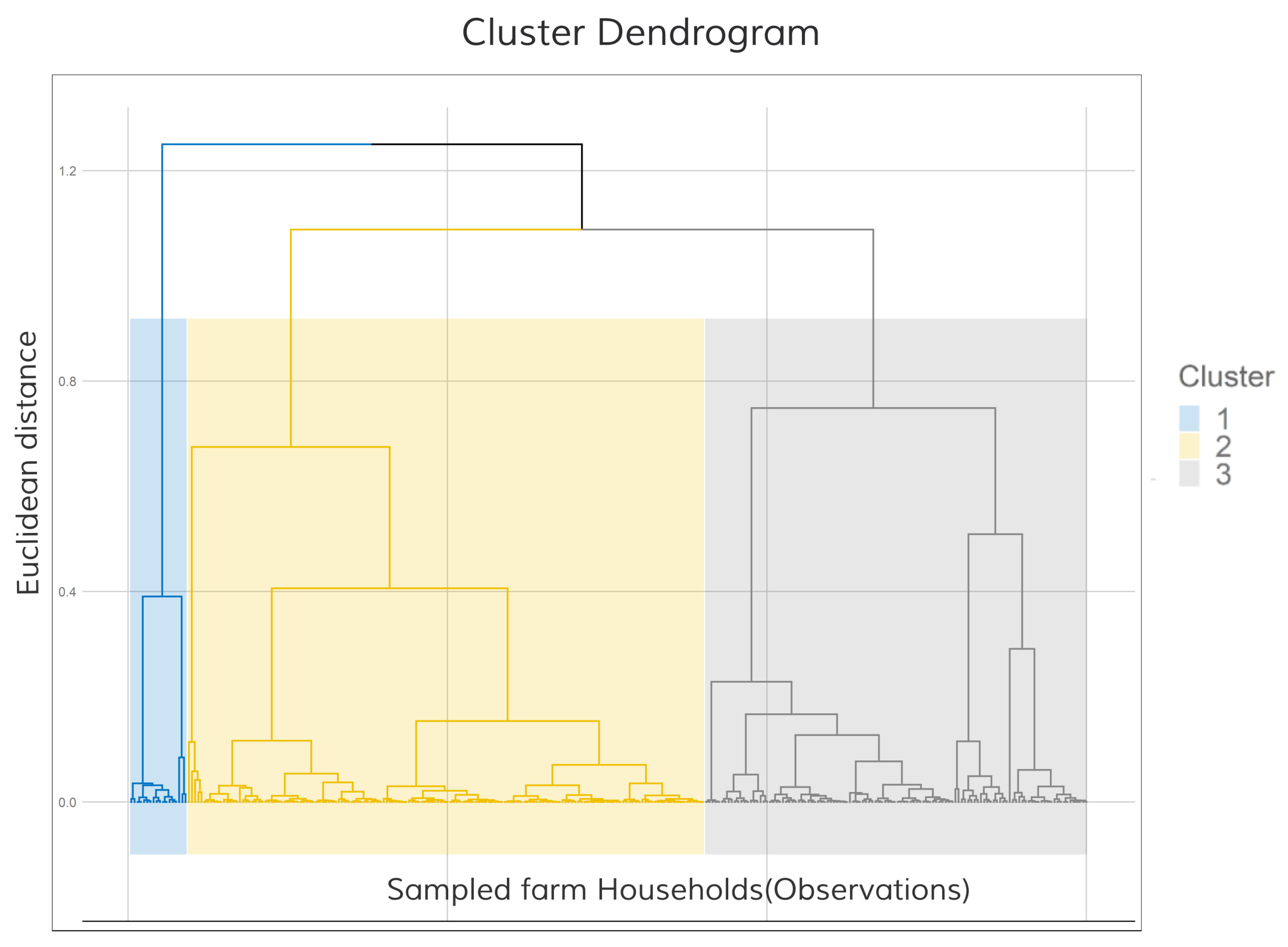
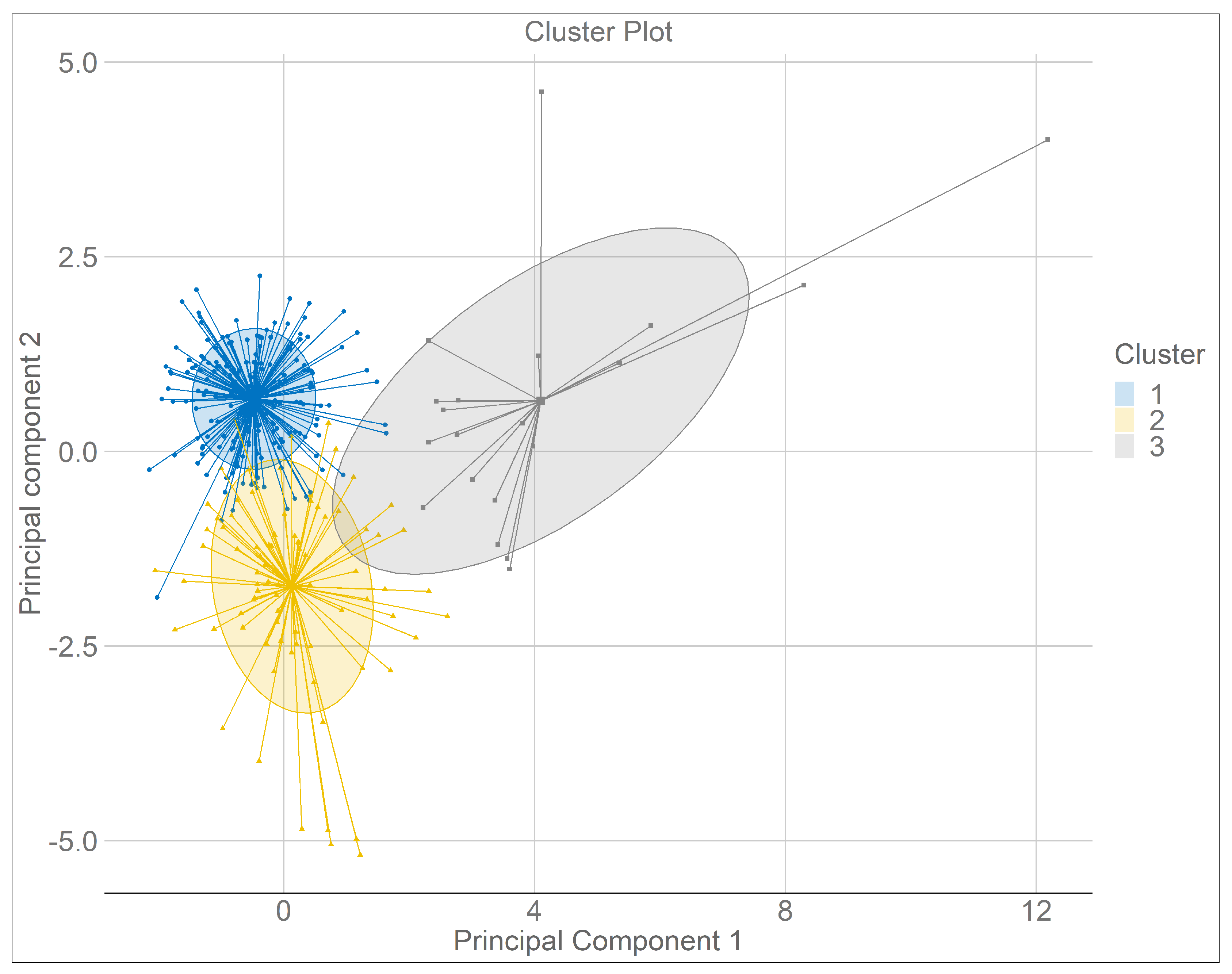
Using the hierarchical and k-means clustering, a three-cluster solution was obtained. Figure 2 provides the tree-based representation of the observation, also known as a dendrogram. Moreover, partitioning in three clusters is represented on the scatter plot produced by the first two principal components, and the dots (representing farmers) are colored according to their cluster group Figure 3. The cluster dendrogram shows explicitly three different farm groups identified by the cluster analysis. Table A1 presents the variables that discriminate each cluster group.
Cluster I accounts for 68.4% of the farm households in KVF. Share of rice, share of hired labor and the household commercialization index are significantly and positively associated with the first cluster. Given the importance of these variables, we labeled the first cluster as “Monocrop rice producers” (MCRPs), with almost 92 percent of their land allocated to rice (compared to 79% for all farmers). Considering the main crop, they tend to have a larger share of hired labor and higher input intensity. Almost 50 percent of their rice harvests are sold to the market to cover the costs of inputs and basic household needs. In terms of livelihood, they are dependent on farm income without livestock integration. They own less land, with an average of 1.97 hectares compared to an average of 2.5 hectares in the study site. Although there is limited off-farm income opportunity, monocrop rice producers also receive income from non-farming activities.
Cluster II accounts for 25.2% of the sampled farm households. Share of land allocated to maize, rice, and vegetables as well as share or hired labor are most significantly associated with cluster two. Hence, we labeled the second cluster of farmers as “Diversifiers”. Diversifiers are different from the other two groups, mainly in terms of their land-use decision. Although the highest share of land is allocated to rice (47%), they also produce maize (40%) and vegetables (10%). Households in this group mainly rely on family labor, with only 24% of the labor provided by wage labor.
Cluster III comprises 6.4% of the farm households. The third cluster is strongly associated with farm size, TLU, household size, and per capita income. Given the mix of farming and livestock keeping, we labeled it as “Agropastoralists”. The Agropastoralists own relatively more land and TLU, have larger household sizes, and earn larger per capita income relative to their peers in the valley. Moreover, they are characterized by lower market participation (crop) and lower labor person-days per year per hectare. Agropastoralists are recently migrated farmers from other parts of the country who have cleared new land for cultivation of crops and livestock keeping. One possible explanation for the lower market participation (commercialization index of 31 compared to the overall average 47) is the large household size, which might require them to keep a significant portion of their output for home consumption.
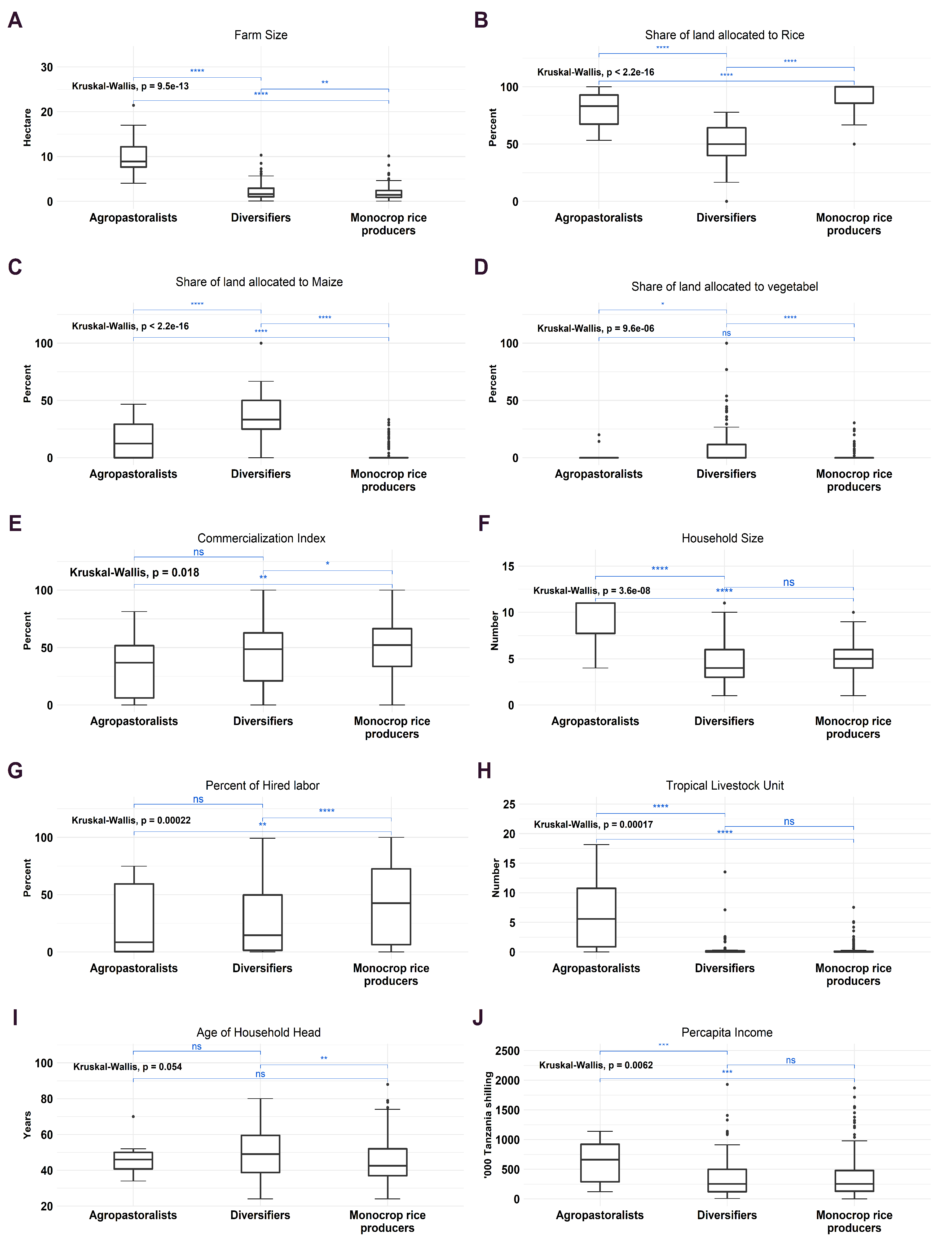
Figure 4 provides the box plots for the characterization of the three farm groups. To test if there is a significant difference between the groups, a pairwise mean comparison is conducted. As shown in the plots, there is a significant difference between the Agropastoralist and Diversifier types in terms of farm size (Figure 4A), land allocated to crops (Figure 4B–D), household size (Figure 4F), TLU (Figure 4H) and per capita income (Figure 4J). Similarly, the results show a significant difference between Agropastoralists and MCRP in terms of farm size (Figure 4A), land allocated to crops (Figure 4B–D), commercialization index (Figure 4E), household size (Figure 4F), share of hired labor (Figure 4G), TLU (Figure 4H) and per capita income (Figure 4J). Looking at the difference between MCRP and diversifiers, there is a significant difference between the two farm groups in farm size (Figure 4A), land allocated to crops (Figure 4B–D), commercialization index (Figure 4E), the share of hired labor (Figure 4G) and age of the household head (Figure 4I).

3.4. Validation of Typology

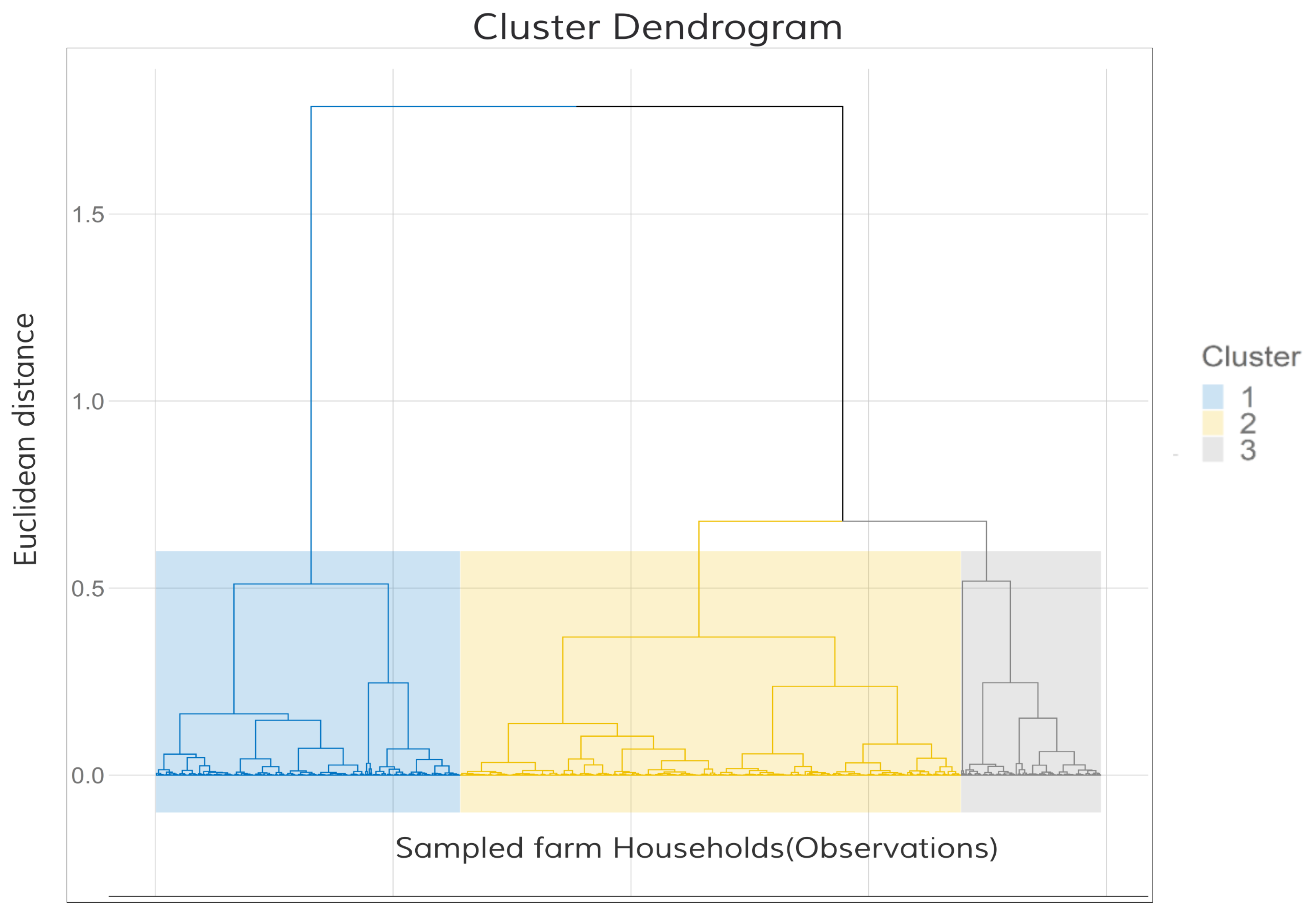
In order to check the validity and stability of the clusters identified above, we conduct a validation exercise using the 2007 Agriculture Sample Survey (ASS) of Tanzania [78]. The data contain 810 observations across 54 villages in the Kilombero and Ulanga districts. The selection of the variables and algorithms are the same as in the above analysis (however, the ASS data miss two important variables: per capita income and amount of labor used in crop production). The typology from the new dataset reveals the same pattern as the one we found from our survey. The same number of clusters are identified(Figure 5), and the main variables that discriminate the clusters are the same (Figure A1). Besides, the typology from the 2007 agricultural sample survey also shows other interesting differences between farm types. For example, the distance of the main farmer field from the river is significantly higher for diversifiers relative to their peers of Monocrop rice producers and Agropastoralists. This might explain why diversifiers can allocate a relatively larger share of land to maize.

4. Discussion

The results presented above provide insight into the heterogeneity among farm households in the KVF. The diversity is observed not only in terms of livelihood and land use but also with respect to resource endowments and market participation. Understanding the diversity of the farmers and how the current policies and strategies are shaping the livelihood of smallholder farmers is key for several reasons: (1) KVF is one of the hotspot areas for agricultural intensification, and interventions from both state and aid funded projects will likely continue to grow. (2) It is an ecologically sensitive area that provides a range of ecosystem services and its sustainable use will have both national and regional benefits [52]. (3) It is one of the largest rice-growing areas in East Africa and rice is one of the vital commodities targeted by both the government and aid agencies for food security and export earnings [5]. (4) Despite the government’s efforts to implement different policy instruments, objectives have not been fully met, and impacts are minimal so far [79].
The current agricultural policy of Tanzania is addressed in several government strategies and policy documents, including the Agriculture Sector Development Programme-II (ASDS-II), KILIMO KWANZA Resolve, the Tanzania Food Security Investment Plan and the Southern Agriculture Growth Corridor of Tanzania (SAGCOT) [2]. ASDS-II and SAGCOT are two agricultural programs with direct implications for KVF. Although the two policy interventions represent different priorities (smallholder farmers and large scale commercial ventures, respectively), both policies envision to increase agricultural production and reduce rural poverty through training and information on agricultural technology by extension services, building infrastructure including small-scale irrigation, road and warehouses, and integration of smallholder farmers into value chains [79].
To date, these policies have tended to ignore the diversity of smallholder farmers, their needs, and constraints [57,80,81]. Effective development strategies and plans seeking to harmonize future food production and environmental sustainability in KVF should be systematically targeted and thus need to take into consideration the challenges and opportunities associated with different farm types. The variety of farm households identified through our typology can form a basis for prioritizing existing policies and for targeting future intervention to a specific farming system. For instance, the ASDS-II has vowed to increase access to agricultural mechanization services, including tractors, power tillers, weeder, and harvesters, etc., in collaboration with the private sector [79] (p. 71). The monocrop rice producer could benefit from such interventions that prioritize access to labor-saving technologies and innovations, as they use significantly more family and wage labor for land preparation, weeding, and harvesting of rice. Although the adoption of more diverse cropping systems depends fundamentally on the hydrological regime of a particular farm, Monocrop rice producers and Agropastoralists could benefit from policies and interventions, targeting a transition towards agroecology through temporal and spatial diversification of cropping practices (rotation, multiple cropping, and intercropping) accompanied by water management practices. This will help them to spread production and income risk over a broader range of crops and to reduce vulnerability to exogenous shocks. Both Monocrop rice producers and Diversifiers earn their income mainly from a single source (crop production). Thus, they could also benefit from efforts towards income diversification into non and off-farm activities and from increased credit access for investing in diversified production systems. Since all the farmers still use traditional farming practices, they could benefit from access to low cost, environmentally friendly, and improved farming technologies, as envisioned in both ASDS-II and SAGCOT [2,82]. This will allow them to increase their productivity, which might in turn reduce the speed and scale of the current transformation of natural ecosystems into agricultural production. Finally, the Agropastoralists have not been actively engaged in the current policy landscape [83] and they require additional attention. Poor infrastructure and insecurity increase the costs and risks of commercialization for Agropastoralists located in remote areas. They are less able to respond to terms of trade and sell less of their surplus production. Interventions through road infrastructure (especially between the isolated settlements and the main road) as envisioned in SAGCOT [84] (p. 19) might benefit Agropastoralists. As conflicts between the Agropastoralist and the crop farmers are increasing in recent years [85], sustainable rangeland management that ensures mobility and connectivity to key natural resources and takes into account the carrying capacity of the floodplain (as foreseen in ASDS-II [82] (p. 21)) might benefit both the farmers and the environment.

5. Conclusions

In this study, we attempted the first classification and characterization of farm households in KVF using cross-sectional data collected in 2015. By combining principal component analysis, hierarchical clustering, and K-means clustering, we segment farmers by a purely data-driven approach into groups exhibiting similarity within and differences between them, based on their livelihood and land use. Moreover, we provide an inductive generalization [27] through a concise characterization of the groups, and assign appropriate meanings to them.
Our result shows an easily comprehensible typology with three representative farm types that capture the main aspects of the heterogeneity. The majority of the farmers in the valley are Monocrop rice producers who are characterized by their higher land allocation to rice, market participation, and labor use. The second farm type identified is called Diversifier. Households in this group are similar to the Monocrop rice producers in some respect, but show a significant difference in terms of using relevant acreage for maize and vegetables in addition to rice. More so, the share of hired labor is relatively small, due to less emphasis on labor-intensive rice production. The third group of farmers is identified as Agropastoralists. Households in this group pursue their livelihood by combining crop production with livestock keeping. Furthermore, they also own significantly more land and have a higher per capita income. Our validation based on a completely independent dataset shows a similar classification and characterization of farmers, which indicates that a combination of PCA, hierarchical, and K-means clustering provides stable clusters. Understanding the diversity of farmers in KVF is essential for any effort geared towards increasing production and the reduction of poverty in the region. Recognition of this diversity may avoid a lack of success and unintended consequences of policy measures caused by ignoring the specific constraints and circumstances of each farm type. Besides, the farm typology will help us to define particular agent types and to appropriately parameterize behavioral models for future research of land use and intensification in KVF.

Author Contributions

Conceptualization, B.H.G.; methodology, B.H.G.; writing—original draft preparation, B.H.G.; writing—review and editing, S.R., T.H.; supervision, T.H., S.R.; funding acquisition, T.H. All authors have read and agreed to the published version of the manuscript.

Funding

This study was supported through The GlobE: Wetlands in East Africa project funded by the German Federal Ministry of Education and Research (FKZ: 031A250 A-H), with additional funding provided by the German Federal Ministry of Economic Cooperation and Development; Deutsche Forschungsgemeinschaft (DFG) under the CRC/Transregio 228: Future Rural Africa: Future-making and social-ecological transformation (Project number: 328966760). SR is funded by the Deutsche Forschungsgemeinschaft (DFG, German Research Foundation) under Germany’s Excellence Strategy - EXC 2070 – 390732324, project PhenoRob.

Conflicts of Interest

The authors declare no conflict of interest.The funders had no role in the design of the study; in the collection, analyses, or interpretation of data; in the writing of the manuscript, or in the decision to publish the results.

Abbreviations

The following abbreviations are used in this manuscript:
SAGCOTSouthern Agricultural Growth Corridor of Tanzania
GOTGovernment of Tanzania
TShTanzanian shelling
KVFKilombero Valley Floodplain
MCRPMonocrop rice producer
PCAPrincipal component analysis
TLUTropical livestock unit
SDStandard deviation
CVCoefficient of variation
GISGeographic information system

Appendix A

Appendix A.1. Table of Discramintory Variables

Table A1. Cluster description by main discriminatory variables.
Cluster MeanOverall MeanCluster SDOverall SDp Value
Cluster I [ Monocrop Rice Producers] [68.4%]
Share of land allocated to rice91.4779.1811.0223.910.00
Percent of labor hired43.4136.8033.6633.130.00
Commercialization index49.8747.0523.4524.750.00
Total labor person-days (ha 1 year 1 )322.11297.39259.15241.170.01
Total expenditure on
Agro-inputs (000 Tsh) (ha 1 )
36.35829.99892.56579.0860.05
Household size4.815.051.641.980.00
Share of land allocated to vegetables1.423.535.2211.510.00
Farm size in Ha1.972.371.512.170.00
TLU0.230.680.672.240.00
Share of land allocated to maize3.4113.857.4121.370.00
Cluster II [Diversifier] [25.2%]
Share of land allocated to maize39.6613.8524.4321.370.00
Share of land allocated to vegetables9.983.5319.8411.510.00
Percent of labor Hired24.4136.8027.4333.130.00
Share of land allocated to rice47.0079.1819.8723.910.00
Cluster III [Agropastoralist] [6.4%]
TLU7.070.685.362.240.00
Farm size in Ha7.672.373.062.170.00
Household size8.445.052.221.980.00
Share of land allocated to maize23.9913.8517.6721.370.04
Total labor person-days (ha 1 year 1 )151.53297.39121.15241.170.01
Years of schooling4.896.443.452.470.01
Commercialization index31.0947.0523.9524.750.00
Percent of labor hired14.8136.8022.8633.130.00

Appendix A.2. Box Plot of Validation Cluster
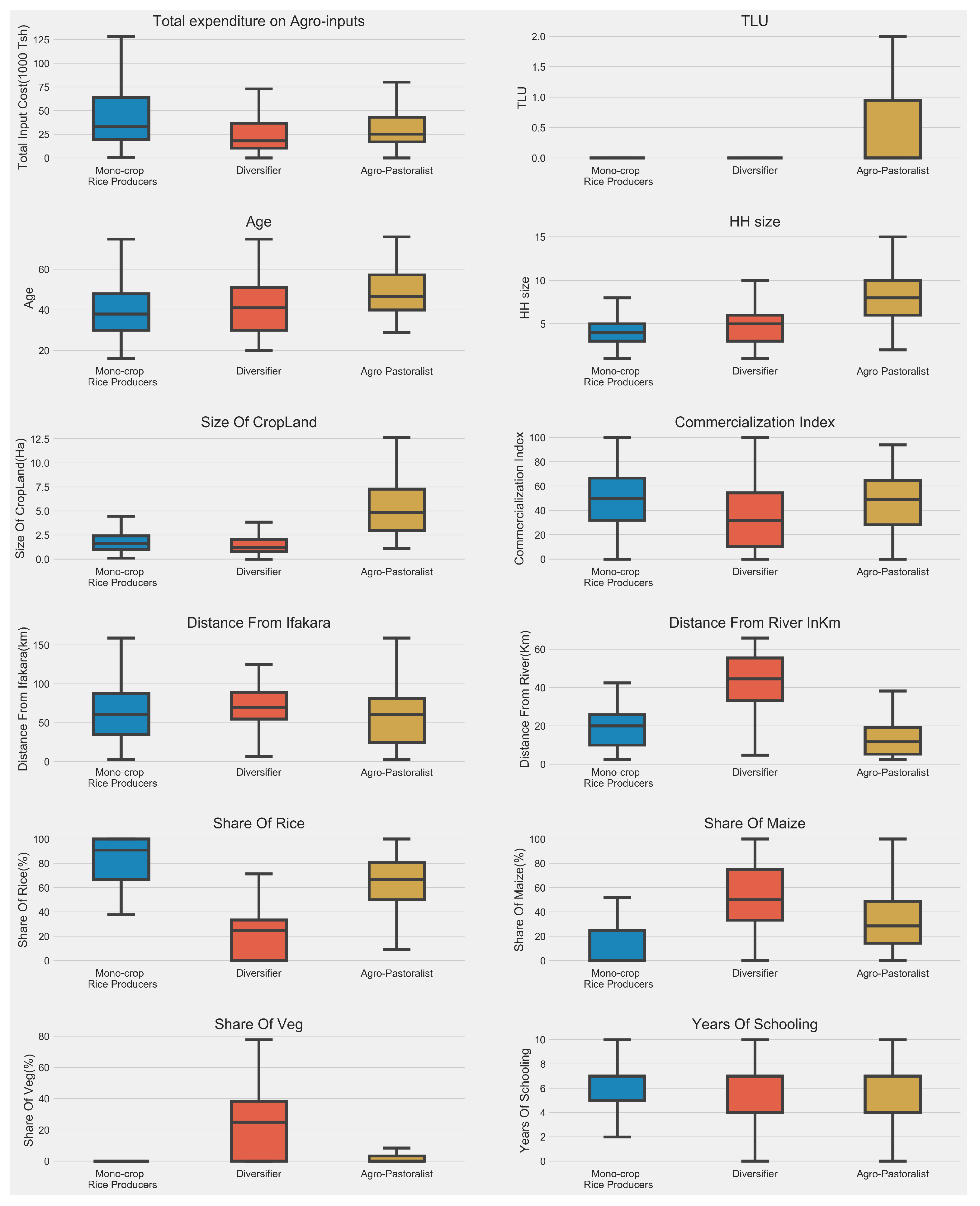
Figure A1. Box plots of main variables by farm type from the validation study (based on the 2007 agricultural Sample census [78]. [n = 800]).
Sustainability 12 07114 g0a1

References

  1. Milder, J.C.; Buck, L.E.; Hart, A. Applying an Agriculture Green Growth Approach in the SAGCOT Clusters: Challenges and Opportunities in Kilombero, Ihemi and Mbarali; Technical Report; SAGCOT Centre: Dar es Salaam, Tanzania, 2013. [Google Scholar]
  2. Environmental Resources Management. Southern Agricultural Growth Corridor of Tanzania (SAGCOT): Strategic Regional Environmental and Social Assessment; RFP Number: A/082/hq/S/Sagt/pmu/7, ERM Project Number: 0159588; Environmental Resources Management: Dar es Salaam, Tanzania, 2012; p. 144. [Google Scholar]
  3. Bamford, A.; Ferrol-Schulte, D.; Smith, H. The Status of the Ruipa Corridor between the Selous Game Reserve and the Udzungwa Mountains; Technical Report; Frontier Tanzania: Dar es Salaam, Tanzania, 2010. [Google Scholar]
  4. Dinesen, L. Kilombero Valley Floodplain (Tanzania). In The Wetland Book: II: Distribution, Description and Conservation; Finlayson, C.M., Milton, G.R., Prentice, R.C., Davidson, N.C., Eds.; Springer Netherlands: Dordrecht, The Netherlands, 2016; pp. 1–8. [Google Scholar]
  5. Kato, F. Development of a major rice cultivation area in the Kilombero Valley, Tanzania. Afr. Study Monogr. 2007, 36, 3–18. [Google Scholar] [CrossRef]
  6. Nindi, S.J.; Maliti, H.; Bakari, S.; Kija, H.; Machoke, M. Conflicts Over Land and Water Resources in the Kilombero Valley Floodplain, Tanzania. Afr. Study Monogr. 2014, 50, 173–190. [Google Scholar]
  7. Kangalawe, R.Y.M.; Liwenga, E.T. Livelihoods in the wetlands of Kilombero Valley in Tanzania: Opportunities and challenges to integrated water resource management. Phys. Chem. Earth 2005, 30, 968–975. [Google Scholar] [CrossRef]
  8. Mombo, F.; Speelman, S.; Kessy, J.; Hella, J.; Van Huylenbroeck, G. Determinants of access patterns to goods and services from wetlands in Tanzania and the impact on sustainable wetland management. Afr. J. Agric. Res. 2012, 7, 5585–5593. [Google Scholar] [CrossRef]
  9. Msofe, N.K.; Sheng, L.; Lyimo, J.; Msofe, N.K.; Sheng, L.; Lyimo, J. Land Use Change Trends and Their Driving Forces in the Kilombero Valley Floodplain, Southeastern Tanzania. Sustainability 2019, 11, 505. [Google Scholar] [CrossRef] [Green Version]
  10. Ronald, B.; Dulle, F.; Honesta, N. Assessment of the Information Needs of Rice Farmers in Tanzania: A Case Study of Kilombero District, Morogoro. Libr. Philos. Pract. e-J. 2014, 1071, 1–33. [Google Scholar]
  11. Jenkins, B. Mobilizing the Southern Agricultural Growth Corridor of Tanzania: A Case Study; The CSR Initiative at the Harvard Kennedy School: Cambridge, MA, USA, 2012. [Google Scholar]
  12. Schnitzer, P.; Azzarri, C. Tanzania Agricultural Snapshot 2007/8; Working Paper; HarvestChoice-International Food Policy Research Institute: Washington, DC, USA, 2014. [Google Scholar]
  13. Martin-Prével, A.; Frédéric, M.; Mittal, A. The Unholy Alliance, Five Western Donors Shape a Pro-Corporate Agenda for African Agriculture; The Oakland Institute: Oakland, CA, USA, 2016; pp. 1–28. [Google Scholar]
  14. Milder, J.C.; Buck, L.E.; Hart, A.K.; Scherr, S.J.; Shames, S.A. A framework for Agriculture Green Growth: Greenprint for the Southern Agricultural Growth Corridor of Tanzania (SAGCOT); SAGCOT Centre: Dar es Salaam, Tanzania, 2013. [Google Scholar]
  15. New Markets Lab; SAGCOT. A Legal Guide to Strengthen Tanzania’s Seed and Input Markets; Alliance for a Green Revolution in Africa (AGRA): Nairobi, Kenya, 2017; p. 148. [Google Scholar]
  16. Mombo, F.; Speelman, S.; Hella, J.; Van Huylenbroeck, G. How characteristics of wetlands resource users and associated institutions influence the sustainable management of wetlands in Tanzania. Land Use Policy 2013, 35, 8–15. [Google Scholar] [CrossRef]
  17. Saravia Matus, S.; Cimpoeis, D.; Ronzon, T. Literature Review and Proposal for an International Typology of Agricultural Holdings; A World Agricultures Watch Report; Food & Agriculture Org.: Rome, Italy, 2013. [Google Scholar]
  18. Dixon, J.A.; Gibbon, D.P.; Gulliver, A. Farming Systems and Poverty: Improving Farmers’ Livelihoods in a Changing World; Food & Agriculture Org.: Rome, Italy, 2001. [Google Scholar]
  19. AGRA. African Agriculture Status Report: Focus on Staple Crops; Technical Report; Alliance for a Green Revolution in Africa (AGRA): Nairobi, Kenya, 2013. [Google Scholar]
  20. AGRA. African Agriculture Status Report: The Business of Smallholder Agriculture in Sub-Saharan Africa(Issue 5); Technical Report; Alliance for a Green Revolution in Africa (AGRA): Nairobi, Kenya, 2017. [Google Scholar]
  21. Garrity, D.; Dixon, J.; Boffa, J.M. Understanding African Farming Systems; Invited paper, Food Security in Africa: Bridging research and Practise; Australian International Food Security Centre: Canberra, Australia, 2012; pp. 1–50. [Google Scholar]
  22. Whitfield, S.; Dixon, J.L.; Mulenga, B.P.; Ngoma, H. Conceptualising farming systems for agricultural development research: Cases from Eastern and Southern Africa. Agric. Syst. 2015, 133, 54–62. [Google Scholar] [CrossRef]
  23. Osabuohien, E.S.; Efobi, U.R.; Herrmann, R.T.; Gitau, C.M. Female labor outcomes and large-scale agricultural land investments: Macro-micro evidencefrom Tanzania. Land Use Policy 2019, 82, 716–728. [Google Scholar] [CrossRef]
  24. Herrmann, R.T. Large-Scale Agricultural Investments and Smallholder Welfare: A Comparison of Wage Labor and Outgrower Channels in Tanzania. World Dev. 2017, 90, 294–310. [Google Scholar] [CrossRef]
  25. Nakano, Y.; Tanaka, Y.; Otsuka, K. Impact of training on the intensification of rice farming: Evidence from rainfed areas in Tanzania. Agric. Econ. 2018, 49, 193–202. [Google Scholar] [CrossRef]
  26. Bidogeza, J.C.; Berentsen, P.B.M.; De Graaff, J.; Oude Lansink, A.G.J.M. A typology of farm households for the Umutara Province in Rwanda. Food Secur. 2009, 1, 321–335. [Google Scholar] [CrossRef]
  27. Gebauer, R.H. Socio-economic classification of farm households—Conceptual, methodical and empirical considerations. Eur. Rev. Agric. Econ. 1987, 14, 261–283. [Google Scholar] [CrossRef]
  28. Guiomar, N.; Godinho, S.; Pinto-Correia, T.; Almeida, M.; Bartolini, F.; Bezák, P.; Biró, M.; Bjørkhaug, H.; Bojnec, S.; Brunori, G.; et al. Typology and distribution of small farms in Europe: Towards a better picture. Land Use Policy 2018, 75, 784–798. [Google Scholar] [CrossRef]
  29. Köbrich, C.; Rehman, T.; Khan, M. Typification of farming systems for constructing representative farm models: Two illustrations of the application of multi-variate analyses in Chile and Pakistan. Agric. Syst. 2003, 76, 141–157. [Google Scholar] [CrossRef]
  30. Goswami, R.; Chatterjee, S.; Prasad, B. Farm types and their economic characterization in complex agro-ecosystems for informed extension intervention: Study from coastal West Bengal, India. Agric. Food Econ. 2014, 2. [Google Scholar] [CrossRef] [Green Version]
  31. Kuivanen, K.S.; Michalscheck, M.; Descheemaeker, K.; Adjei-Nsiah, S.; Mellon-Bedi, S.; Groot, J.C.J.; Alvarez, S. A comparison of statistical and participatory clustering of smallholder farming systems—A case study in Northern Ghana. J. Rural Stud. 2016, 45, 184–198. [Google Scholar] [CrossRef]
  32. Takeshima, H.; Nin-Pratt, A.; Diao, X.; Nin-Pratt, A.; Diao, X.; Nin-Pratt, A.; Diao, X. Mechanization and agricultural technology evolution, agricultural intensification in Sub-Saharan Africa: Typology of agricultural mechanization in Nigeria. Am. J. Agric. Econ. 2013, 95, 1230–1236. [Google Scholar] [CrossRef] [Green Version]
  33. Valbuena, D.; Verburg, P.H.; Bregt, A.K. A method to define a typology for agent-based analysis in regional land-use research. Agric. Ecosyst. Environ. 2008, 128, 27–36. [Google Scholar] [CrossRef]
  34. Berre, D.; Corbeels, M.; Rusinamhodzi, L.; Mutenje, M.; Thierfelder, C.; Lopez-Ridaura, S. Thinking beyond agronomic yield gap: Smallholder farm efficiency under contrasted livelihood strategies in Malawi. Field Crops Res. 2017, 214, 113–122. [Google Scholar] [CrossRef]
  35. Kuivanen, K.S.; Alvarez, S.; Michalscheck, M.; Adjei-Nsiah, S.; Descheemaeker, K.; Mellon-Bedi, S.; Groot, J.C. Characterising the diversity of smallholder farming systems and their constraints and opportunities for innovation: A case study from the Northern Region, Ghana. NJAS-Wagen. J. Life Sci. 2016, 78, 153–166. [Google Scholar] [CrossRef]
  36. Pacini, G.C.; Colucci, D.; Baudron, F.; Righi, E.; Corbeels, M.; Tittonell, P.; Stefanini, F.M. Combining multi-dimensional scaling and cluster analysis to describe the diversity of rural households. Exp. Agric. 2014, 50, 376–397. [Google Scholar] [CrossRef] [Green Version]
  37. Pienaar, L.; Traub, L.N. Understanding the Smallholder Farmer in South Africa: Towards a Sustainable Livelihoods Classification. In Proceedings of the 29th International Conference on Agricultural Economics, Milan, Italy, 8–14 August 2015; International Association of Agricultural Economists: Milan, Italy, 2015. [Google Scholar]
  38. Tittonell, P.; Muriuki, A.; Shepherd, K.; Mugendi, D.; Kaizzi, K.; Okeyo, J. The diversity of rural livelihoods and their influence on soil fertility in agricultural systems of East Africa—A typology of smallholder farms. Agric. Syst. 2010, 103, 83–97. [Google Scholar] [CrossRef]
  39. Andersen, E.; Elbersen, B.; Godeschalk, F.; Verhoog, D. Farm management indicators and farm typologies as a basis for assessments in a changing policy environment. J. Environ. Manag. 2007, 82, 353–362. [Google Scholar] [CrossRef]
  40. Daloglu, I.; Nassauer, J.I.; Riolo, R.L.; Scavia, D. Development of a farmer typology of agricultural conservation behavior in the american corn belt. Agric. Syst. 2014, 129, 93–102. [Google Scholar] [CrossRef]
  41. Hazeu, G.W.; Metzger, M.J.; Mücher, C.A.; Perez-Soba, M.; Renetzeder, C.; Andersen, E. European environmental stratifications and typologies: An overview. Agric. Ecosyst. Environ. 2011, 142, 29–39. [Google Scholar] [CrossRef]
  42. Nin-Pratt, A.; ElDidi, H.; Breisinger, C. Farm Households in Egypt: A Typology for Assessing Vulnerability to Climate Change; MENA RP Working Paper 12; International Food Policy Research Institute (IFPRI): Washington, DC, USA; Cairo, Egypt, 2018; 53p. [Google Scholar]
  43. Shukla, R.; Agarwal, A.; Sachdeva, K.; Kurths, J.; Joshi, P. Climate change perception: An analysis of climate change and risk perceptions among farmer types of Indian Western Himalayas. Clim. Chang. 2019, 152, 103–119. [Google Scholar] [CrossRef]
  44. Wezel, A.; Casagrande, M.; Celette, F.; Vian, J.F.; Ferrer, A.; Peigné, J. Agroecological practices for sustainable agriculture. A review. Agron. Sustain. Dev. 2014, 34, 1–20. [Google Scholar] [CrossRef] [Green Version]
  45. Therond, O.; Duru, M.; Roger-Estrade, J.; Richard, G. A new analytical framework of farming system and agriculture model diversities. A review. Agron. Sustain. Dev. 2017, 37, 21. [Google Scholar] [CrossRef]
  46. Alvarez, S.; Paas, W.; Descheemaeker, K.; Tittonell, P.; Groot, J. Typology Construction, a Way of Dealing with Farm Diversity General Guidelines for Humidtropics; Report for the CGIAR Research Program on Integrated Systems for the Humid Tropics; Plant Sciences Group, Wageningen University: Wageningen, The Netherlands, 2014; pp. 1–37. [Google Scholar]
  47. Hansen, P.; Jaumard, B. Cluster analysis and mathematical programming. Math. Program. 1997, 79, 191–215. [Google Scholar] [CrossRef] [Green Version]
  48. Husson, F.; Le, S.; Pages, J. Exploratory Multivariate Analysis by Example Using R; A CHAPMAN & HALL BOOK: New York, NY, USA, 2017; p. 248. [Google Scholar]
  49. Alvarez, S.; Timler, C.J.; Michalscheck, M.; Paas, W.; Descheemaeker, K.; Tittonell, P.; Andersson, J.A.; Groot, J.C.J. Capturing farm diversity with hypothesis-based typologies: An innovative methodological framework for farming system typology development. PLoS ONE 2018, 13, e0194757. [Google Scholar] [CrossRef] [PubMed] [Green Version]
  50. Le, Q.B.; Park, S.J.; Vlek, P.L.G. Land Use Dynamic Simulator (LUDAS): A multi-agent system model for simulating spatio-temporal dynamics of coupled human-landscape system. 2. Scenario-based application for impact assessment of land-use policies. Ecol. Inform. 2010, 5, 203–221. [Google Scholar] [CrossRef]
  51. Villamor, G.B.; van Noordwijk, M.; Le, Q.B.; Lusiana, B.; Matthews, R.; Vlek, P.L.G. Diversity deficits in modelled landscape mosaics. Ecol. Inform. 2011, 6, 73–82. [Google Scholar] [CrossRef]
  52. Wilson, E.; Mcinnes, R.; Mbaga, P.; Ouedraogo, P. Kilombero Valley, United Republic of Tanzania: Ramsar Advisory Mission Report; Technical Report; The Ramsar Convention Secretariat: Gland, Switzerland, 2017. [Google Scholar]
  53. Lyon, S.W.; Koutsouris, A.; Scheibler, F.; Jarsjö, J.; Mbanguka, R.; Tumbo, M.; Robert, K.K.; Sharma, A.N.; van der Velde, Y. Interpreting characteristic drainage timescale variability across Kilombero Valley, Tanzania. Hydrol. Process. 2015, 29, 1912–1924. [Google Scholar] [CrossRef]
  54. Ntongani, W.A.; Munishi, P.K.T.; More, S.R.; Kashaigili, J.J. Local Knowledge on the Influence of Land Use/Cover Changes and Conservation Threats on Avian Community in the Kilombero Wetlands, Tanzania. Open J. Ecol. 2014, 4, 723. [Google Scholar] [CrossRef] [Green Version]
  55. RAMSAR. Information Sheet on Ramsar Wetland: The Kilombero Valley Floodplain; The Ramsar Convention Secretariat: Gland, Switzerland, 2002; pp. 1–17. [Google Scholar]
  56. Munishi, P.K.T.; Chuwa, J.J.; Kilungu, H.; Moe, S.R.; Temu, R.P.C. Management Effectiveness and Conservation Initiatives in the Kilombero Valley Flood Plains Ramsar Site, Tanzania. Tanzan. J. For. Nat. Conserv. 2012, 81, 1–10. [Google Scholar]
  57. KILORWEMP. Technical Advisory Services for Biodiversity Conservation and Wetland Management in Kilombero Valley RAMSAR Site, Tanzania:Pastoralism Diagnostic Study; Technical Report; KILORWEMP Project Implementation Unit: Dar es Salaam, Tanzania, 2017. [Google Scholar]
  58. Blache, A. Grabbing Land, Catching Votes! Land and the 2015 Election Campaign in Kilombero District, Tanzania. East Afr. Rev. 2020, 53. Available online: http://journals.openedition.org/eastafrica/791 (accessed on 31 August 2020).
  59. National Bureau of Statistics. 2012 Population and Housing Census; Population Distribution by Adminstrative Areas; National Bureau of Statistics: Dar es Salaam, Tanzania, 2013.
  60. MALF. Tanzania Livelihood Baseline Profile: Kilombero-Ulanga-Lusewa Paddy, Maize, and Cassava Livelihood Zone; Zone Discription 43; Ministry of Agriculture Livestock and Fisheries— Agriculture Department: Dar es Salaam, Tanzania, 2015.
  61. Jones, T.; Bamford, A.J.; Ferrol-Schulte, D.; Hieronimo, P.; McWilliam, N.; Rovero, F. Vanishing Wildlife Corridors and Options for Restoration: A Case Study from Tanzania. Trop. Conserv. Sci. 2012, 5, 463–474. [Google Scholar] [CrossRef]
  62. Jun, C.; Ban, Y.; Li, S. China: Open access to Earth land-cover map. Nature 2014, 514, 434. [Google Scholar] [CrossRef] [Green Version]
  63. Scoones, I. Sustainable Rural Livelihood: A Framework For Analysis IDS WORKING PAPER 72; IDS: Brighton, UK, 1998. [Google Scholar]
  64. Iraizoz, B.; Gorton, M.; Davidova, S. Segmenting farms for analysing agricultural trajectories: A case study of the Navarra region in Spain. Agric. Syst. 2007, 93, 143–169. [Google Scholar] [CrossRef]
  65. Schmitzberger, I.; Wrbka, T.; Steurer, B.; Aschenbrenner, G.; Peterseil, J.; Zechmeister, H. How farming styles influence biodiversity maintenance in Austrian agricultural landscapes. Agric. Ecosyst. Environ. 2005, 108, 274–290. [Google Scholar] [CrossRef]
  66. Takeshima, H.; Edeh, H. Typology of Farm Households and Irrigation Systems: Some Evidence from Nigeria. Ssrn 2013. [Google Scholar] [CrossRef] [Green Version]
  67. Takeshima, H. Understanding Irrigation System Diversity in Nigeria: A Modified Cluster Analysis Approach. Irrig. Drain. 2016, 65, 601–612. [Google Scholar] [CrossRef]
  68. Singh, C.; Dorward, P.; Osbahr, H. Developing a holistic approach to the analysis of farmer decision-making: Implications for adaptation policy and practice in developing countries. Land Use Policy 2016, 59, 329–343. [Google Scholar] [CrossRef]
  69. Lacoste, M.; Lawes, R.; Ducourtieux, O.; Flower, K. Assessing regional farming system diversity using a mixed methods typology: The value of comparative agriculture tested in broadacre Australia. Geoforum 2018, 90, 183–205. [Google Scholar] [CrossRef]
  70. Dunteman, G.H. Principal Components Analysis; Number 69; SAGE Publications, Inc.: Newbury Park, CA, USA, 1989. [Google Scholar]
  71. Hair, J.F., Jr.; Black, W.C.; Babin, B.J.; Anderson, R.E. Multivariate Data Analysis, 7th ed.; Essex CM20 2JE; Pearson Education Limited: London, UK, 2014; pp. 1–739. [Google Scholar]
  72. Husson, F.; Josse, J.; Pages, J. Principal Component Methods—Hierarchical Clustering—Partitional Clustering: Why Would We Need to Choose for Visualizing Data? Technical Report 1; Applied Mathematics Department: Rennes, France, 2010. [Google Scholar] [CrossRef]
  73. Everitt, B.S.; Landau, S.; Leese, M.; Stahl, D. Cluster Analysis 5th Addition2011, 5th ed.; John Wiley & Sons, Ltd. Registered: West Sussex, UK, 2011; p. 848. [Google Scholar] [CrossRef]
  74. Härdle, W.K.; Simar, L. Applied Multivariate Statistical Analysis; Pearson: Upper Saddle River, NJ, USA, 2013; pp. 1–516. [Google Scholar] [CrossRef]
  75. Le, S.; Josse, J.; Husson, F. FactoMineR: An R Package for Multivariate Analysis. J. Stat. Softw. Artic. 2008, 25, 1–18. [Google Scholar] [CrossRef] [Green Version]
  76. Kassambara, A.; Mundt, F. Factoextra: Extract and visualize the results of multivariate data analyses. R Package Version 2016, 1, 337–354. [Google Scholar]
  77. R Core Team. R: A Language and Environment for Statistical Computing; R Foundation for Statistical Computing: Vienna, Austria, 2018. [Google Scholar]
  78. TNBS. National Sample Census of Agriculture 2007/08; Tanzania National Bureau of Statistics: Dar es selaam, Tanzania, 2009; Volume V, pp. 1–345.
  79. Government of Tanzania. National Agriculture Policy; Technical Report; Ministry of Agriculture Food Security and Cooperatives: Dar es selaam, Tanzania, 2016.
  80. NRGF. Natural Resource Governance in Kilombero Cluster and the SAGCOT INITIATIVE: An Assessment of Key Issues and Recommendations for Action; Technical Report; CEESP and IUCN: Gland, Switzerland, 2017. [Google Scholar]
  81. Wineman, A.; Jayne, T.S.; Isinika Modamba, E.; Kray, H. The changing face of agriculture in Tanzania: Indicators of transformation. Dev. Policy Rev. 2020. [Google Scholar] [CrossRef]
  82. URT. Agricultural Sector Development Strategy-II 2015/2016–2024/2025; Technical Report; United Republic of Tanzania: Dar es selaam, Tanzania, 2016.
  83. URT. (SAGCOT) Investment Project Public Notice. Re-Disclosure of Environmental and Social Management Framework (ESMF); Technical Report; Prime Minister’s Office: Dar es selaam, Tanzania, 2011.
  84. AgDevCo.; Prorustica. Southern Agricultural Growth Corridor of Tanzania Investment Blueprint; Technical Report; AgDevCo.: Dar es selaam, Tanzania, 2011. [Google Scholar]
  85. Bergius, M.; Benjaminsen, T.A.; Maganga, F.; Buhaug, H. Green economy, degradation narratives, and land-use conflicts in Tanzania. World Dev. 2020, 129, 104850. [Google Scholar] [CrossRef]
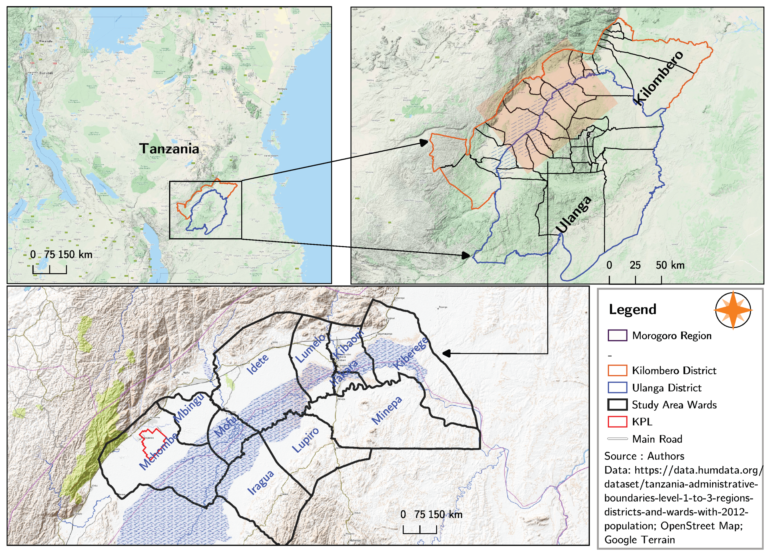
Figure 1. Location of study site.
Sustainability 12 07114 g001
Figure 2. Dendrogram of three farm types in KVF. Note: The cluster dendrogram is the standard ways of representing the hierarchical relations and allocation of samples in to groups. The cluster is based on agglomerative hierarchical clustering with Euclidean distance as the similarity measure and Ward’s linkage strategy (n = 300).
Sustainability 12 07114 g002
Figure 3. Distribution of the farmer household in three groups projected on the one and two dimensional plane. Note: Principal component 1 and 2 are the first two components from PCA that capture 30.33% of the variation.
Sustainability 12 07114 g003
Figure 4. Box plots of farmer characterization in KVF by main variables. Note: The horizontal lines between the box plots shows if there is significant differences in mean of a particular variable between groups (pairwise mean comparison) at different significant levels [ns: p > 0.05] [*: p <= 0.05] [**: p <= 0.01] [***: p <= 0.001] [****: p <= 0.0001]. Kruskal–Wallis test is a non-parametric test to compare samples from two or more groups of independent observations, p < 0.05 is considered as significant.
Sustainability 12 07114 g004
Figure 5. Dendrogram of three farm types in KVF (validation data). Note: The cluster is based on agglomerative hierarchical clustering with Euclidean distance as the similarity measure and Ward’s linkage strategy. The validation is based on data from Agriculture Sample Survey (2007) [78] (n = 800).
Sustainability 12 07114 g005
Table 1. Descriptive statistics for the variables included in typology constructions.
VariableDescriptionUnitMean
(SD)
CV
AgeThe age of the household headyears46.53
(12.92)
0.28
Household sizeNumber of individuals in the householdnumber5.12
(2.15)
0.42
Share of ricePercentage of the total cultivated
land allocated to rice
%78.77
(23.93)
0.3
Share of maizePercentage of the total cultivated
land allocated to maize
%13.92
(21.19)
1.52
Farm sizeThe size of farm land ownedha2.61
(2.78)
1.06
TLUTotal Tropical livestock unitTLU1.46
(6.56)
4.49
Percent hiredShare of labor hired%37.25
(33.21)
0.89
Commercialization indexAn index of commercializationindex47.05
(24.8)
0.53
Expenditure on Agro-inputsOverall input intensity, measured as
the total value of inputs (Fertilizer, seed
and agro-chemicals) (ha 1 )
TSh64,984.41
(349,645.18)
5.38
Distance riverDistance from plot to the nearest riverkm2.61
(3.68)
1.41
Off Farm incomePercentage of Income from non-farm
sources
%9.78
(21.74)
2.22
Share of VegetablePercentage of the total cultivated
land allocated to vegetables
%3.8
(11.92)
3.14
Per capita incomePer capita income per yearTSh (000)516.37
(1124.84)
2.18
Total labor person daysTotal labor use in the farm (ha 1 )Man-days317.36
(337.07)
1.06
Years of schoolingTotal number of years in schoolyears6.37
(2.56)
0.4
Note: SD = Standard Deviation; CV = Coefficient of Variation; TSh = Tanzanian shilling; ha 1 = per hectare; n = 300.
Table 2. Six principal components with loading, eigenvalues and cumulative explained variance.
VariablesCorrelation between a Variable and a Principal Component
PC1PC2PC3PC4PC5PC6
Age of household head0.40870.0818−0.25880.0385−0.6458−0.1076
Household size0.56340.34910.07770.15780.2715−0.1077
Share of land allocated to rice−0.48390.7854−0.33240.0160.03160.0328
Share of land allocated to maize0.5246−0.66340.2328−0.20040.22370.1673
Farm size owned in Ha0.53280.4320.42650.06020.1217−0.1854
Tropical livestock unit0.55910.31990.00820.290.33210.0207
Share of hired labor−0.47720.15360.48610.054−0.1049−0.2018
Commercialization index−0.4606−0.11680.08230.36720.2311−0.3844
Total expenditure in agro-inputs (000 Tsh)−0.20820.00560.21580.6280.04950.2937
Distance from the nearest river in Km0.0882−0.06910.18540.5091−0.06910.4159
Share of Off farm income−0.11430.16560.4908−0.2506−0.29080.2696
Share of land allocated to vegetables−0.0153−0.37910.33490.4172−0.394−0.3816
Income per capita−0.0780.28690.5297−0.1394−0.16020.4079
Total labor person days per year−0.3336−0.2853−0.42290.18840.15350.3579
Years of schooling−0.4332−0.12940.4455−0.28710.3907−0.1092
Eigenvalues2.232.011.571.281.191.02
Cumulative explained variance1630.3341.5650.7259.2766.56
Note: The bold values identify the top three strongly correlated variables with the respective PC.