Integral Application of Chemical Mass Balance and Watershed Model to Estimate Point and Nonpoint Source Pollutant Loads in Data-Scarce Little Akaki River, Ethiopia

Abstract

The quality of Little Akaki River in Addis Ababa (Ethiopia) is deteriorating significantly due to uncontrolled waste released from point and diffuse sources. In this study, pollution load from these sources was quantified by integrating chemical mass balance analysis (CMB) and the watershed model of pollution load (PLOAD) for chemical oxygen demand, biochemical oxygen demand, total dissolved solid, total nitrogen, nitrate, and phosphate. Water samples monitored bimonthly at 15 main channel monitoring stations and 11-point sources were used for estimation of pollutant load using FLUX32 software in which the flow from the soil and water assessment tool (SWAT) model calibration, measured instantaneous flow, and constituent concentration were used as input. The SWAT simulated the flow quite well with a coefficient of determination (R²) of 0.78 and 0.82 and Nash-Sutcliff (NSE) of 0.76 and 0.80 during calibration and validation, respectively. The uncharacterized nonpoint source load calculated by integrating CMB and PLOAD showed that the contribution of nonpoint source prevails at the middle and downstream segments of the river. Maximum chemical oxygen demand (COD) load from uncharacterized nonpoint sources was calculated at the monitoring station located below the confluence of two rivers (near German Square). On the other hand, high organic pollution load, biochemical oxygen demand (BOD) load, was calculated at a station upstream of Aba Samuel Lake, whereas annual maximum total dissolved solid (TDS), total nitrogen (TN), and phosphate load (PO₄-P) from the nonpoint source in Little Akaki River (LAR) were found at a river section near Kality Bridge and maximum NO_X load was calculated at station near German Square. The integration of the CMB and PLOAD model in this study revealed that the use of area-specific pollutant export coefficients would give relatively accurate results than the use of mean and median ECf values of each land use.

1. Introduction

Nowadays, urban rivers of developing countries are heavily polluted due to the release of pollutants from the point and nonpoint sources where the determination of accurate pollution load to a river is often difficult due to combined factors of financial, data quality and availability, and technical capability making the river water quality management more challenging [1]. In one way, not only is the determination of waste load from various sources, such as diffuse sources, difficult to quantify as a result of complexity in the generation and uneven distribution of wastewater from various sources [2], but also as a result of the lack of clear distinction between urban point and diffuse pollution sources [3]. On the other hand, pollutants released from point sources such as industries and institutions to the rivers are becoming a threat to the aquatic life arising from poor waste load allocation and monitoring systems, and most importantly, monitoring all the point sources in a watershed is quite difficult due to economic and time limitations [4]. Despite the wide range of challenges for the estimation of pollutant loads on different watersheds, scientists have tried to develop different approaches and come up with various best pollution management practices. The most common approaches for pollutants load estimation are based on watershed models that require extensive data, which were reported in the works of [5,6,7,8]. Similarly, the application of the land use-based pollutant export coefficient method [9] and the modified mass balance approach [10] are also alternative pollutant load estimation techniques. Researchers often recommend the study of pollutant loads rather than the concentration could ease the river pollution and pollutant load management in a river system [11].

When the data required for the estimation of pollutant loads are limited, it is often necessary to explore simple approaches that estimate the transport of loads from various land uses to water [1]. Various researchers have hence used different techniques to estimate pollutant loads from diffuse sources. One such approach, which has been widely used, is through the determination of pollutant flux based on the base flow separation [12]. However, such an approach could not be feasible for data-scarce areas like Ethiopia, which has little hydrometeorological and water quality data. Availability of monitored water quality and hydrological data is central for the accurate determination of the pollutant load that hence hinders the urban water quality management and pollution load estimation, specifically in developing worlds. In that case, an indirect approach, such as chemical mass balance (CMB) analysis, which is often considered as an economical and viable way, is used as a means of preliminary load estimation. Waseem et.al. [13] recommended the use and importance of detailed information of water and chemical mass balance analysis approach for the establishment of efficient surface and ground water management. However, the CMB approach for pollutant load estimation is more accurate if the time of travel between the river segments of monitoring stations is small and the river is assumed to be completely mixed. Many studies have been conducted to estimate the pollutant loads in a river using the CMB analysis. The application of CMB was used by Raj et.al. [14] to determine the subsurface flow contribution to a river where the load difference between the monitoring stations nearby was that contributed by the flow from a subsurface source. The method was also used for the estimation of internal processes in rivers, sediments, and chemical resuspension [15], where bottom sediment usually plays a key role by acting as both source/sink during mass flux and CMB analysis [16]. The approach was also used as a means of preliminary pollutant lateral load estimation in different watersheds such as in India [17], North America [18], and Europe [15].

In Ethiopia, due to combined limitations of finance, monitoring data, and commitment, it is nowadays becoming difficult to estimate loads from point and nonpoint sources, and hence river water quality management is neglected. However, the recent initiation of the government to reduce the point source pollution has led the nonpoint source pollution to be recognized, and it has ultimately become the primary focus area. It is apparent that pollutant load estimation specifically originating from nonpoint sources in data-scarce catchments like Ethiopia is challenging. Thus, the use of less complex, effective, economical, and reliable watershed models is highly important for better pollutant load estimation in river water quality management. Therefore, the objectives of this research were: quantification of annual pollutant loads contributions from point and nonpoint sources to the Little Akaki River (LAR), to identify the possible pollution load hotspots, and calibration of pollutant export coefficient for the study area by integrating CMB analysis and catchment nonpoint source model of pollution load (PLOAD).

2. Materials and Methods

2.1. The Study Area

Addis Ababa is the sprawling city and capital, economic, and political center of Ethiopia, found on the border of the greater rift valley at the foothill of the Entoto mountain, with a total land area of 520 square kilometers and population of more than 3 million [19]. The study area (Figure 1) is characterized by a subtropical highland climate with a mean annual maximum and minimum temperature of 24 °C and 12 °C, respectively, and a mean monthly rainfall of 260 mm [20]. The main surface water sources of the city consist of three rivers: Kebena River, Big Akaki River (BAR), and Little Akaki River (LAR), all originating at the foothills of Entoto and draining down to Aba Samuel Lake. The LAR flows from the northwest of the city to the most southern Addis Ababa, before joining the BAR at Aba Samuel Lake, and has a total length of 43 km. The LAR consists of several highly polluted tributaries, mainly located in the middle of the catchment where untreated household waste, including raw sewage, and industrial waste that increases pollution load in the river are discharged. Nearly 65% of the country’s industries, ranging from small-scale to large-scale, are concentrated in and around Addis Ababa [21], including food and beverage, textiles, tanneries, rubber, and paper products. The location of most large-scale industries within the vicinity of the LAR that are releasing their wastewater directly to the river without prior treatment (more than 90%) has augmented the pollution load, making the river’s water quality unmanageable easily [22]. The river is serving as a natural sewer line for waste originating from various sources, such as domestic, industrial, institutional, and residential areas [23]. The study area is characterized by trachytes, rhyolites, basalts, and several episodes of pyroclastic materials of older volcanic rocks, specifically prevailing in the upper catchments, whereas the western, southwestern, and eastern parts of Addis Ababa are characterized by younger volcanic of trachy-basalt.

2.2. Water Quality Sampling and Flow Simulation

A bimonthly water sample was collected for selected constituents in LAR from April 2018 to March 2019 during dry and wet seasons. A total of 11 physico-chemical parameters were collected and analyzed where dissolved oxygen (DO), water temperature, pH, total dissolved solids (TDS), and conductivity were determined onsite. For the estimation of pollutant load in LAR, water samples were collected from 15 main channel monitoring stations (

Table 1. Main channel monitoring stations and locations in LAR.

Code	Station Name	Longitude	Latitude	Area (ha)
M1	LAR at Medhanealem Square	38°43′14″	9°03′10.1″	277.15
M2	LAR near Kolfe Atena Tera Taiwan Sefer	38°43′3.1″	9°02′38.3″	74.31
M3	LAR at the Back of Coca Cola SC	38°43′38″	9°00′53.1″	437.14
M4	LAR downstream of AACRA	38°44′21″	8°59′55.5″	343.59
M5	LAR near Kera Beg Tera	38°44′44″	8°59′12.7″	400.42
M6	LAR Downstream of Likuanda Bridge	38°42′7.1″	9°02′2.13″	1202.13
M7	LAR Upstream of Alert Hospital at Augusta	38°42′35″	8°59′18.5″	461.62
M9	LAR at German Square	38°44′5.1″	8°57′57.3″	826.42
M10	LAR Upstream of Biheretsige Park	38°44′57″	8°57′28.6″	476.48
M11	LAR Downstream of Biheretsige Park	38°45′32″	8°56′58.7″	294.63
M12	LAR Downstream of Batu Tannery	38°45′45″	8°55′50.1″	777.23
M13	LAR at Kality Bridge	38°44′44″	8°54′15.4″	869.91
M14	LAR Upstream of Aba Samuel Lake	38°44′53″	8°52′51.8″	1870.96
M15	LAR Downstream of Addis Ababa Tannery	38°41′20″	9°02′19.7″	9795.4

) and 11 tributaries and point sources (Figure 1 and

Table 2. Identified point sources near LAR, station locations, flow rates, and characteristics.

PS †	Longitude	Latitude	Q	Characteristics
T2	38°43′6.6″	9°3′8.11″	172.8	A tributary with wastewater from Ethio-marble industry
T3	38°43′35″	9°1′7.81″	259.2	A tributary receiving waste mainly from domestic sources
AWF	38°43′39″	9°0′47.4″	95.01	Wastewater originating from wine factory
T4	38°44′24″	9°0′39.6″	518.4	A tributary carrying hospital and tobacco factory waste
AA_Kerawoch	38°44′51″	8°59′16″	362.9	Receive wastewater effluent from abattoirs
T6	38°43′56″	8°57′12″	18144	A tributary carrying agricultural and industrial waste
T5	38°44′59″	8°57′32″	363.04	Small but heavily polluted Kera stream
W_TAN	38°45′30″	8°56′0.6″	181.4	Waste effluent from tannery factory
B_TAN	38°45′30″	8°56′0.6″	267.8	Waste effluent from tannery factory
AA_WWTPE	38°45′9.5″	8°54′51″	4542.4	Addis Ababa waste water treatment plant effluent
M8	38°43′9.6″	8°58′57″	22982.6	Major tributary load
T1	38°43′37.1″	9°3′49.2″	86.3	Very small but highly polluted tributary

^† Point source; Q is the mean flow rate (m³/d).

). The samples were collected using a 1.5 L polyethylene bottle, placed in a cooler box, kept under 4 °C, and immediately transported to the laboratory for analysis. Samples of nitrate and phosphate were prefiltered at site and kept in a cooler box before analysis. The analytical methods and instruments used for analysis are shown in

Table 3. Analytical techniques used for the analysis of selected constituents in LAR.

No	Parameter	Analytical Method	Apparatus/Equipment
1	BOD	Modified Winklers Method	BOD Incubator
2	TDS	Digital Multiparameter	HQ40d
3	COD	Titrimetric	COD Digester, Heating Block
4	PO4-P	Spectrophotometric	HACH DR-2800
5	NOx	Spectrophotometric	UV-VIS Spectrophotometer
6	TKN	Kjeldahl Method	Kjeldahl

. All the analytical methods were done according to the standard methods for the examination of water and wastewater [24].

On the other hand, instantaneous flow in LAR was measured at the time of sample collection using the current meter (Dentan CM-1AX, Tokyo, Japan), and the gauge data for soil and water assessment tool (SWAT) model calibration were collected from the Ministry of Water, Irrigation, and Electricity. The SWAT model calibrated on Big Akaki River (BAR) outlet was used to simulate and generate flow at each of the subcatchment outlets (monitoring stations) and later used for pollutant load calculation at monitoring stations, along with the instantaneous flow and constituent concentration. The flow generated by SWAT for each subcatchment outlet was later input to the FLUX32 software for load estimation at each monitoring station.

2.3. CMB Analysis and Uncharacterized Nonpoint Source Load

In urban rivers of developing countries, the nonpoint source load estimation is a bit challenging due to uncontrolled and irregular waste release rates and unknown and uneven distribution of diffuse sources entry points [25,26,27,28]. To overcome such complexities, various software nowadays are developed to estimate the pollutant loads in a river by taking advantage of simple mathematical equations, from where the diffuse source loads are estimated. FLUX32 is one such software system, developed by the Minnesota Pollution Control Agency (MPCA) to estimate the pollutant loads carried by tributaries and streams. The software requires two data sets: event-based pollutant concentration and respective instantaneous flow and historical gauge recording or model output of the river flow for the specified period [1]. The software uses six different methods to calculate the pollutant load/flux and the choice of each method depends on the sampling approach and variability of flow and concentration [29]. Accordingly, method six (regression applied to individual daily flows) was selected for load calculation in LAR (Equation (1)).

$${\mathrm{W}}_{\mathrm{i}}={{\displaystyle \sum }}^{ }\exp [\mathrm{a}+\left(\mathrm{b}+1\right)\ln \left({\mathrm{Q}}_{\mathrm{i}}\right)+\frac{{\mathrm{SE}}^2}{2}]$$

(1)

where Q_i = mean flow on day i (m³/s), ci = measured constituent concentration (mg/L), a = intercept of ln(c) vs. ln(q) regression, b = slope of ln(c) vs. ln(q) regression, ${\mathrm{SE}}^2$ = standard error of estimate for ln(c) vs. ln(q) regression and q is instantaneous flow (m³/s), W_i = pollutant load/flux (kg/yr).

In LAR, point source load, such as from industries, was calculated by the product of the average discharge rate of wastewater effluents and the mean concentration, where similar approach was used by Amaya et.al. [30], whereas the load from tributaries was calculated by using FLUX32. This is partly because the point source load is often assumed stable and insignificant change occurs seasonally [31,32]. On the other hand, estimation of nonpoint source loads from available monitored water quality data is quite complex and in LAR it was calculated by using upstream–downstream CMB analysis integrating with the watershed model, PLOAD. Since it was difficult to explicitly estimate the nonpoint source load in LAR directly, the term uncharacterized nonpoint source load was used instead, which might include unidentified point source and unrecognized nonpoint source load, where a similar description was used by Jain et.al. [17]. A simple upstream–downstream mass balance approach could be used as an initial estimation of pollution load from lateral sources [33]. Accordingly;

$${\displaystyle \sum } {\mathrm{Q}}_{\mathrm{D}}{\mathrm{C}}_{\mathrm{D}} -{\displaystyle \sum } {\mathrm{Q}}_{\mathrm{Ui}}{\mathrm{C}}_{\mathrm{Ui}} +{\displaystyle \sum } \mathrm{Losses}={{\displaystyle \sum }}^{ }{\mathrm{L}}_{\mathrm{i}}$$

(2)

where Q_D = river flow at the downstream station, C_D = downstream constituent concentration, Q_Ui = flow of a river at a river section upstream, C_Ui = upstream constituent concentration, Σ Losses = the sum of all losses in the stream, L_i = is the net load.

The above simple approach was used in LAR lateral diffuse pollutant load (differential load) estimation for two basic reasons. First, the span length between the monitoring stations is very small, indicating that the loss is minimum and hence neglected. Second, the river constituents are assumed completely mixed. In the above simple mathematical mass balance equation (Equation (2)), the term ΣLi does not mean it is only contributed from nonpoint source loads and is not the exact net load at a point, but the combination of all loads and the losses and/or generations [34], which could be due to settlement, resuspension, and decay and the generation due to reaction.

2.4. Watershed Model Selection

The study of pollutant loads contributing to the pollution of a river is vital for better water quality management. Sekhar et.al. [34] suggested that the catchment pollution management plan should follow a complete study of three components: point sources, nonpoint (background) sources, and natural processes. Though the estimation of point source load is relatively easy, it is challenging to quantify diffuse source loads, specifically in developing countries, where the estimation is often based on simple empirical equations with limited hydro-meteorological and water quality data. To fill such gaps, many watershed models have been developed and studies were conducted to determine pollutant loads from diffuse sources at catchment scale such as the hydrological simulation program—FORTRAN (HSPF) [35], agricultural nonpoint source pollution model (AGNPS) [36], pollution load (PLOAD) [37], soil and water assessment tool (SWAT) [38], and storm water management model (SWMM) [25]. However, most of the models developed so far are complex and require a large number of data, and hence are not feasible for data-scarce areas like Ethiopia. However, watershed level nonpoint source pollution management could be achieved by using a simple but reliable and relatively accurate model with a reasonable and limited budget. In LAR, hence, we used the PLOAD model due to its versatility, simple data usage, and ease of applicability for the study area [1], integrating with the CMB analysis approach based on monitored water quality data. Most researchers prefer the use of PLOAD due to its cheaper and faster water pollution management of water bodies [2] and the capability and adaptability of the model in different watersheds [39]. On the other hand, Zinabu et.al. [1] recommended the use of the PLOAD model in Ethiopia for nonpoint source pollution management.

The PLOAD is a BASINS (better assessment science integrating point and nonpoint sources) model plugin used to estimate nonpoint source load at catchment level interpreted as an annual load [40]. The model integrates point source and GIS-based land-use data to estimate the nonpoint sources’ load contribution from each land use using two approaches: the export coefficient and simple method. Both approaches can be applied based on the data availability and applicability on a watershed, but generally the simple method is used in smaller watersheds, usually less than 1 square mile, while the export coefficient method is used in a mixed land uses [41] for the estimation of constituents such as total suspended solid (TSS), TDS, BOD, COD, NO_x (nitrate + nitrite), total Kjeldahl Nitrogen (TKN), ammonia, feacal coliforms (FC), lead, and zinc [40]. In LAR, we used the export coefficient approach where pollutant loads in PLOAD are calculated by

$${\mathrm{L}}_{\mathrm{p}}={{\displaystyle \sum }}_{\mathrm{P}}({\mathrm{L}}_{\mathrm{PU}}\times {\mathrm{A}}_{\mathrm{U}})$$

(3)

where L_p = pollutant load (kg/yr), L_PU = pollutant export coefficient for each land use (kg/ha/yr), A_U = area by certain land use, ha.

2.5. Pollutant Export Coefficient

The export coefficient (ECf) is the total amount of pollutant load transported from certain land use per unit area over a specified period of time [42]. When estimating catchment nonpoint source contribution by ECf, each land use is assumed to contribute to the pollutant load per land area and is hence expressed in kg/ha/yr. The watershed shape file was delineated by using ArcSWAT, where the land use in the study area is mostly dominated by urban and agricultural set-ups where informal settlements prevail (Figure 2). Accordingly, urban land use has the highest percentage coverage with 51.8%, followed by agricultural land (25.72%), forest (10.18%), rangeland (7.2%), bare land (4.63%), and water (0.46%).

Mathematically, the pollutant load using export coefficient with an inclusion of precipitation induced pollution can be expressed by

$${\mathrm{L}}_{\mathrm{i},\mathrm{j}}={\displaystyle \sum }_{\mathrm{k}=1}^{\mathrm{n}}\left({\mathrm{E}}_{\mathrm{k},\mathrm{i}}\times {\mathrm{A}}_{\mathrm{k},\mathrm{j}}+{\mathrm{P}}_{\mathrm{i},\mathrm{j}}\right)$$

(4)

where L_i,j is calculated load of constituent i at the subcatchment outlet j (kg/yr); n is the number of land uses contributing; E_k,i is the export coefficient of land use k for the constituent i (kg/ha/yr); A_k,j is the area of land use k for the subcatchment j; P_i,j is precipitation-induced constituent i load at a subcatchment j (kg/yr). P_i,j is assumed negligible in LAR.

Availability of the local pollutant export coefficient is a prerequisite for accurate determination of pollutants loads in a watershed. However, the study area did not have an established pollutant ECf and determination for LAR depends on the data on another watershed elsewhere with nearly similar hydrological, topographical, land use, and climatic set-up. To account for catchment variability and to select appropriate ECf values, we evaluated coefficients globally (

Table 4. Export coefficient from literature (kg/ha/yr) selected for pollution load (PLOAD) calibration in LAR.

Land Use	Pollutants Export Coefficient of Different Land Uses from Literature, kg/ha/yr
	TN	TDS	BOD	COD	NOx †	PO4-P
Urban	4.38–36.86 a	292–2263 a	2199.6 e	2343.4 e	91.44 e	1.73 s
Agriculture	2.1–79.6 d	2280 e	68.4 e	90.9 p	34.32 e	9 r
Forest	0.9–38 s	250 j	50 n	50 n	2.12 s	0.71 s
Bare land	0.51–6 b	100 n	3.46 q,o	1–5 *	67.29 r	4.81 r
Water	21.96–73.45 h	10–150 n	50 n	50 n	0.46 s	10.11 r
Rangeland	3.2–14 b	24.02–100.99 j	0.5 s,g	0.5 s,g	0.46 s	2 r,g
	Export coefficients selected for PLOAD calibration in LAR, kg/ha/yr
	TN	TDS	BOD	COD	NOx †	PO4-P
Urban	36	2260	2195	2340	91	1.7
Agriculture	79	2250	68	90	34	9
Forest	38	250	50	50	2	0.70
Bare land	6	100	3.4	5	67	4.8
Water	73	150	50	50	0.45	10
Rangeland	14	100	0.5	0.5	0.45	2

^a [48]; ^e [46]; ^s [11]; ^p [47]; ^b [1]; ^h [26]; ^j [43]; ^r [49]; ^q [40]; * Approximated from PLOAD user guide for BOD [40]; ^d [41]; ⁿ [30]; ^† reported in literature as NO₃ + NO₂; ^r,g estimated from grassland value [49]; ^s,g estimated from grassland value [11]; ^q,o value taken for open land from PLOAD user guide [40].

). For pollutant ECf in PLOAD, we reviewed literature values from Ethiopia [1], Canada [43], USA [41], China [26], Taiwan [44], New Zealand [45], Philippines [30], Egypt [46], Lithuania [47], and Japan [11]. Table 4 summarizes the ECf for pollutants and nutrients in literature and selected for LAR for preliminary estimation.

2.6. Calibration and Validation of PLOAD

PLOAD uses GIS-based input data such as land use, watershed boundary, pollutant loading rate (ECf), rainfall depth and optional best management practices (BMPs), terrain imperviousness, and point sources load based on the type of the approach used for estimation. In PLOAD, nonpoint sources from each land use were calculated based on the ECf for each land use. In LAR, once the ECf for each land use was assigned, the PLOAD was calibrated by using the uncharacterized nonpoint source load calculated by CMB analysis and validated using another set of data using an optimized ECf and measured nonpoint load through CMB. The PLOAD model performance was then evaluated by comparing the measured pollutant load (CMB analysis) with the model output until the total percentage error between the measured and model-predicted value became zero or close to zero. Since the model has no direct calibration option, an Excel (2016)-based optimization on Excel Solver was used. In the Excel Solver, the objective to be optimized was set to minimize the percentage total relative error with a possibility of zero value. We selected a GRG nonlinear optimization in Solver due to its faster performance, which uses the local optimum solution. Accordingly, the performance of the model was checked by;

$$\% \mathrm{ES}=\frac{\mathrm{MPL} - \mathrm{PPL}}{\mathrm{MPL}}$$

(5)

where ES is an error of estimation, MPL is measured pollutant load, PPL is PLOAD predicted load.

3. Results and Discussion

The results in this section are presented in a way that the pollutant load for selected segments of the LAR and monitoring stations of the catchment outlets are represented. The discussion mainly focuses on the major pollution hotspots in the watershed and the pollutant contribution of various land uses were quantified.

3.1. Point Sources Load in LAR

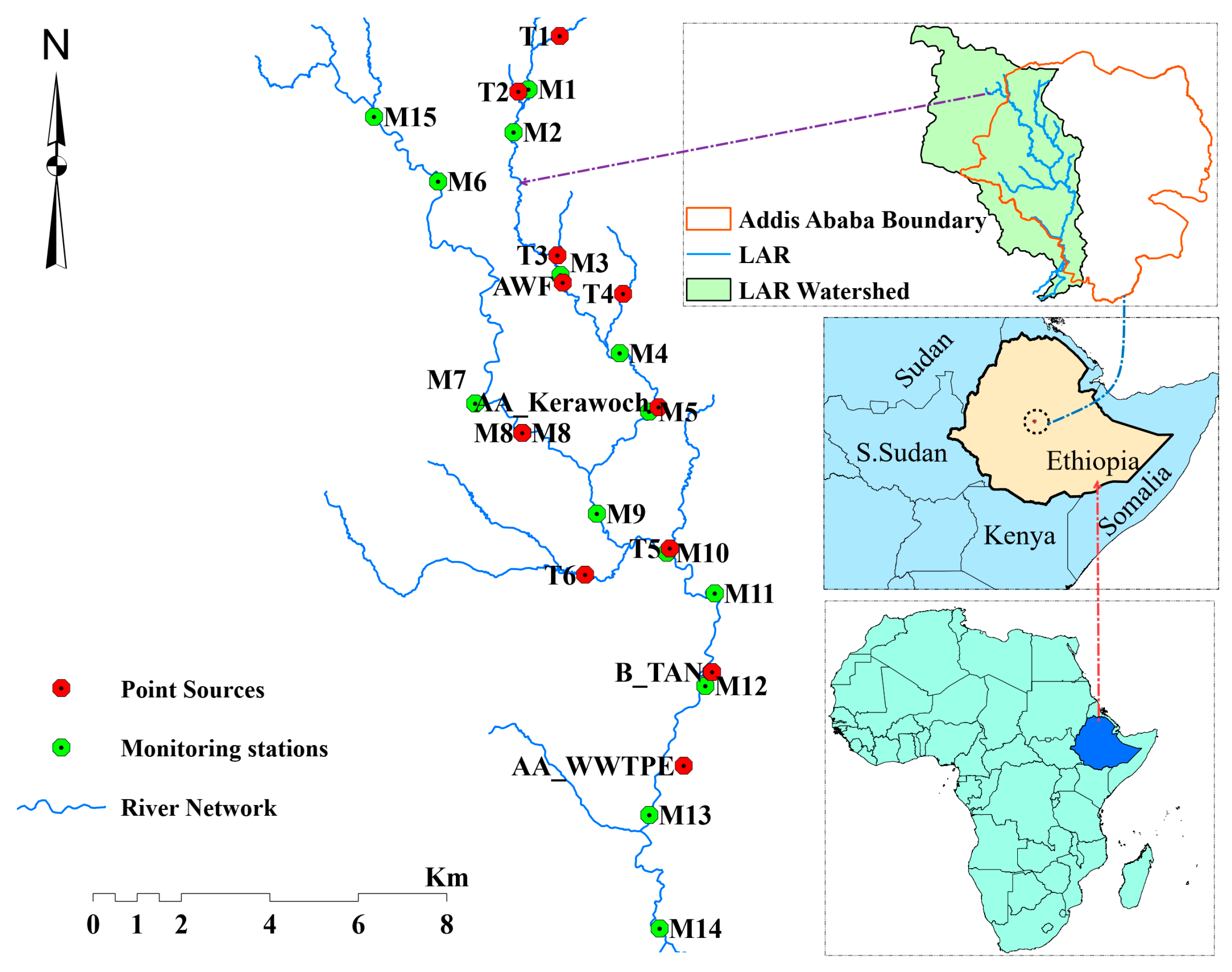
The pollutant load from point sources in LAR was much smaller than the tributaries load due to the relatively higher flow rate and pollution level of the tributaries than the point sources. However, stations M3 to M11 (Figure 1) were heavily loaded by point source pollution that contributes significant pollutant loads to LAR including, the soft drink industry, wine industry, abattoir, tobacco factory, and hospitals. Similarly, the heavily polluted Mesalemya stream that joins the main river upstream of outlet M3 and a tributary that crosses densely populated urban center, Merkato, and receives many wastewaters from industries joining the main river at M4 have highly augmented the pollutant load in LAR. Besides, the load contributed by the Addis Ababa Abattoir near Kera Beg Tera (M5) was found to be very high due to significantly higher water consumption from the slaughterhouse that generates wastewater with a higher flow rate.

Table 5. Summary of point source loads of selected physico-chemical constituents in LAR (t/yr).

Point Source	MS †	Constituents Load in LAR (t/yr)
		COD	BOD	NOx	PO4-P	TDS	TN
T2	M2	37.73	8.32	0.017	0.312	26.52	2.48
T3	M3	185.74	59.89	0.013	1.388	89.75	14.74
AWF	M4	13.69	6.39	0.12	0.447	33.76	0.585
T4	M4	189.45	98.28	0.056	1.180	178.36	10.18
AA_Kerawoch	M5	821.20	105.96	0.073	3.338	306.68	5.298
T6	M10	2867.46	1005.59	1.39	26.20	3185.59	342.65
T5	M10	341.95	98.13	0.115	3.999	358.87	22.07
W_TAN	M12	60.75	3.48	0.740	0.616	49.42	7.076
B_TAN	M12	27.32	14.53	1.912	1.767	103.46	7.617
AA_WWTPE	M13	622.17	217.12	1.005	8.137	440.96	147.26
M8	M9	11,661.75	1052.19	16.35	15.50	5874.30	223.04
T1	M1	82.624	19.99	0.023	0.584	42.69	5.275

MS ^† is downstream monitoring station where the point source load is contributing; T = tributary; AA = Addis Ababa; WWTPE = wastewater treatment plant effluent; M = main channel.

summarizes the load contributed by point sources to the LAR. Almost all of the point sources near LAR discharging the wastewater directly to the river have either no treatment plant or couldn’t fully operate. From the point source load summary on Table 5, it can be apparently seen that the contribution of stations T6, AA_Kerawoch, AA_WWTPE, and M8 were quite significant for the LAR organic and nutrient pollution.

3.2. Flow Simulation and Pollutants Flux in LAR

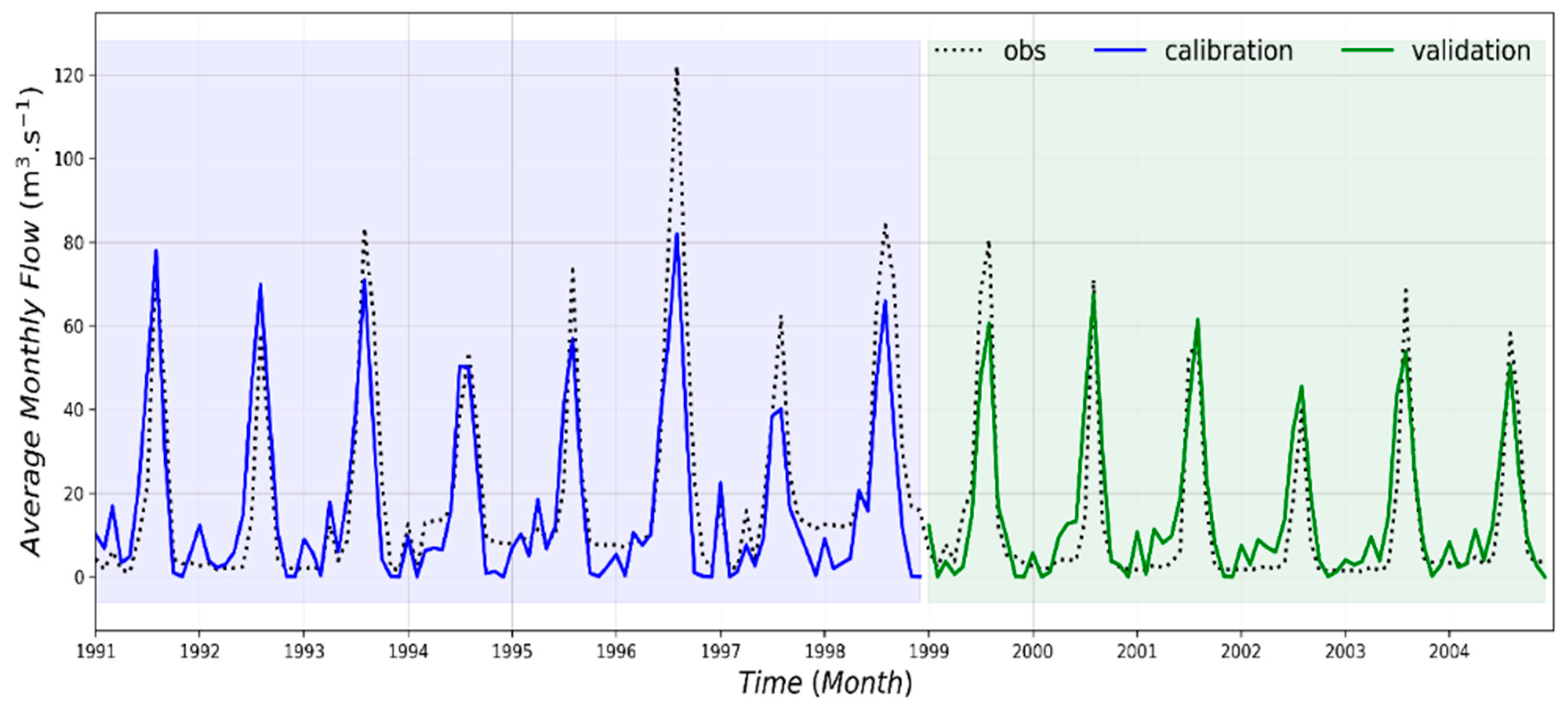
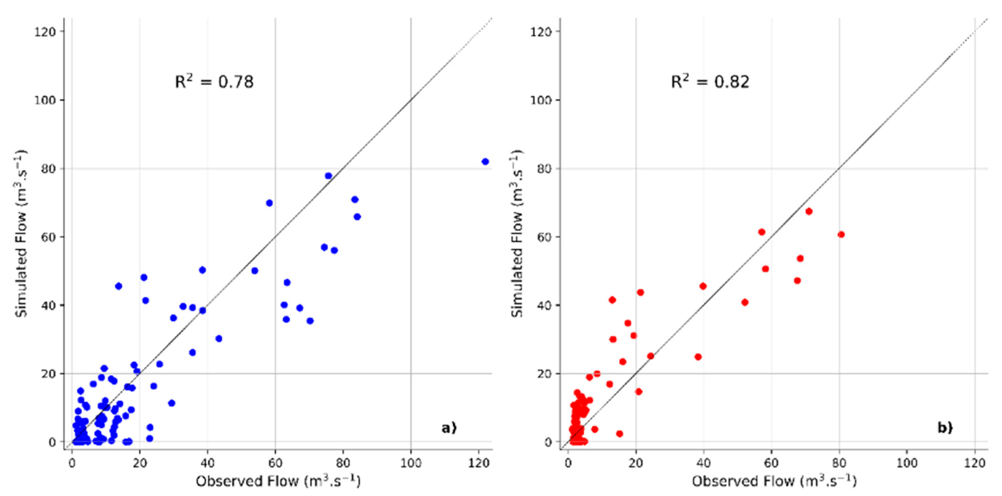
The SWAT calibrated at BAR was used to generate flow in LAR subcatchment outlets where the model output along with the instantaneous flow and constituent concentration was used in FLUX32 software to calculate the pollutant flux (load). Accordingly, the SWAT simulated the flow quite well in Figure 3 and Figure 4 with an R², NSE, and RSR value of 0.78, 0.76, and 0.49 during calibration and 0.82, 0.8, and 0.45 during validation, respectively. The model performance indicators above (R², NSE and RSR) were good enough to interpret the model output for any purpose. From Figure 3, it can be seen that the deviation between the SWAT model simulated and observed peaks. This could primarily be due to the model performance. The hydrological model performance determined by the Nash-Sutcliff (NSE) was found to be 0.76 and 0.78 during calibration and validation in the study area, which is good enough to interpret the model output [50] and the deviation between the observed and simulated flow is interpreted by the error. Similar results were reported elsewhere with similar trends between the model simulation and observation in the works of Abbaspour et.al. [51], Rostamian et.al. [52], and Shawul et.al. [53]. Sometimes the time lag between the small rainfall event and the main rain event could dictate the variation between the model simulation and observed values. This explanation is supported by the study conducted by Li et.al. [35], who used hydrological and water quality model, HSPF, where a similar trend with this study between the model simulated and observed flow was observed. The spatial location of rain meters and the heterogeneity among rainfall stations could also determine the deviation. Though there was deviation between model simulated and observed values at some peak points, the model performance indicators (specifically the Nash-Sutcliff) could suggest that the model output can be interpreted with a good accuracy. The SWAT-generated subcatchment outlet flow was used to calculate the load in FLUX32. Accordingly, the flow-weighted concentration calculated by method 6 (Equation (1)) was < ±20% of all other methods in FLUX32. The residual plot of bias (as slope) for flow, date, and month at each catchment outlet in LAR was in the range of 0–0.05, which is quite acceptable. Similarly, the plot of slope significance was in the range of 0.88–0.99 ≈ 1. The coefficient of variation (CV) is recommended to be in the range of 0–0.2 during flow-weighted load calculation and in LAR, the CV has resulted in the range of 0.03–0.101, which is quite good. During pollutant load calculation in LAR using FLUX32, the presence of the outlier was checked statistically by testing the significance level, p ≤ 0.05.

3.3. Chemical Mass Balance and Pollutants Differential Load in LAR

Once the loads were calculated at each of the subcatchment outlets by FLUX32, a CMB analysis was performed following an upstream–downstream mass balance approach (Equation (2)) to determine the differential load. A similar approach was also followed by [33,34,54]. From the calculated CMB analysis at each monitoring station (

Table 6. Uncharacterized (differential) nonpoint source pollutants load at LAR monitoring stations, chemical mass balance (CMB) analysis.

Pa	Catchment Outlet Differential Load, t/yr
	M1	M2	M3	M4	M5	M9	M10	M11	M12	M13	M14
BOD	27.8	12.7 †	269.69	94.15 †	51.9	1833.2	1867.49 †	738.49 †	395.15	157.65 †	1007.76 †
COD	181.6	87.7	471.93	108.8	65.5	5588.7	1859.55	3228.62 †	2306.9	3217.2	192.12
NOx *	0.05	0.04 †	0.61	0.18	0.04	6.05 †	15.11	2.15 †	10.59n†	0.17	6.10
PO4	0.72	0.12 †	0.43	0.24	1.99	12.43	13.92	7.46	23.63	11.79	7.82 †
TDS	80.7	6.60	162.18	54.06	36.8	581.9	59.67 †	558.85	730.78	1916.2	389.62
TN	1.77	5.39	10.22	11.38 †	15.92	157.2	674.79	97.02	708.88 †	227.65 †	76.82

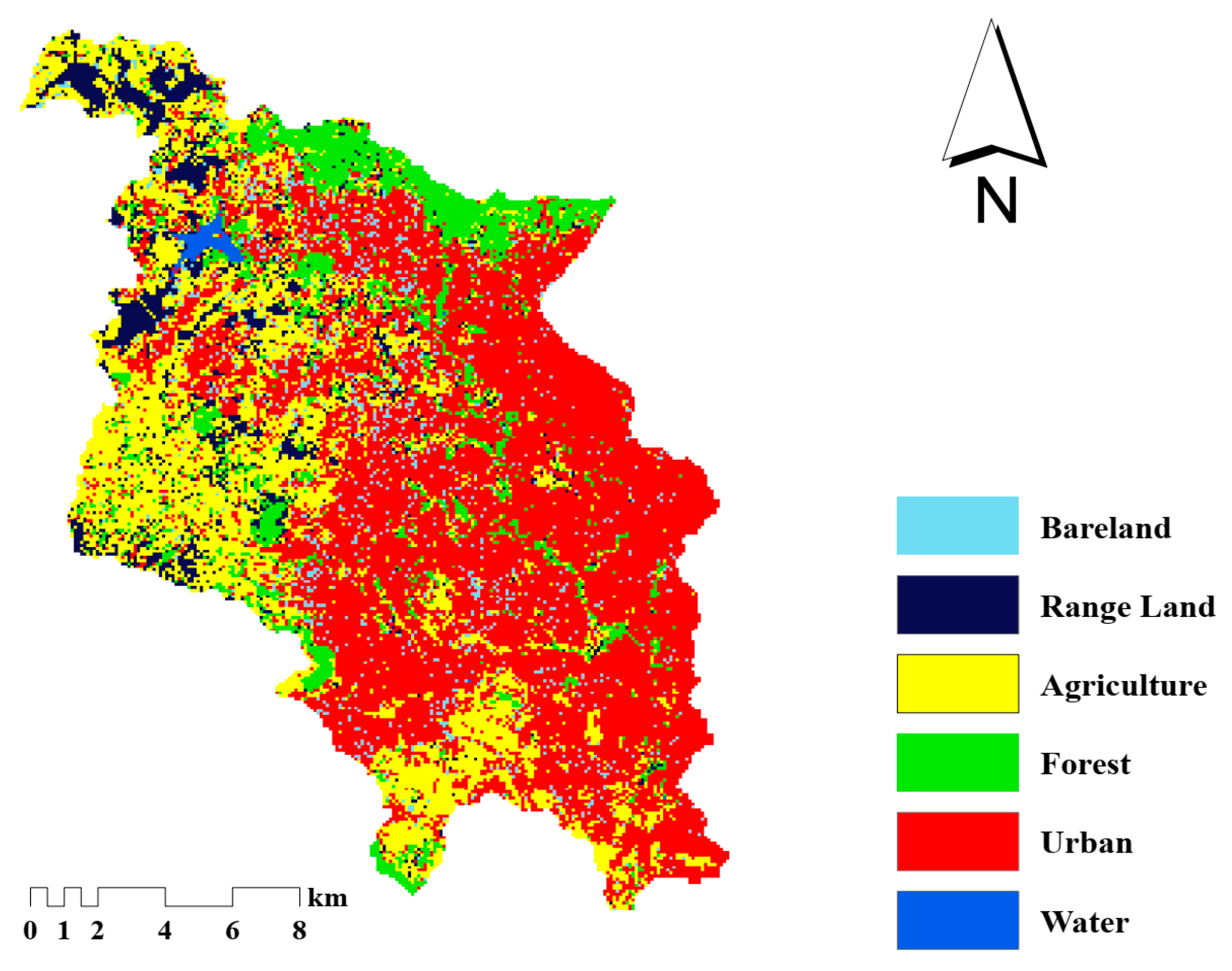
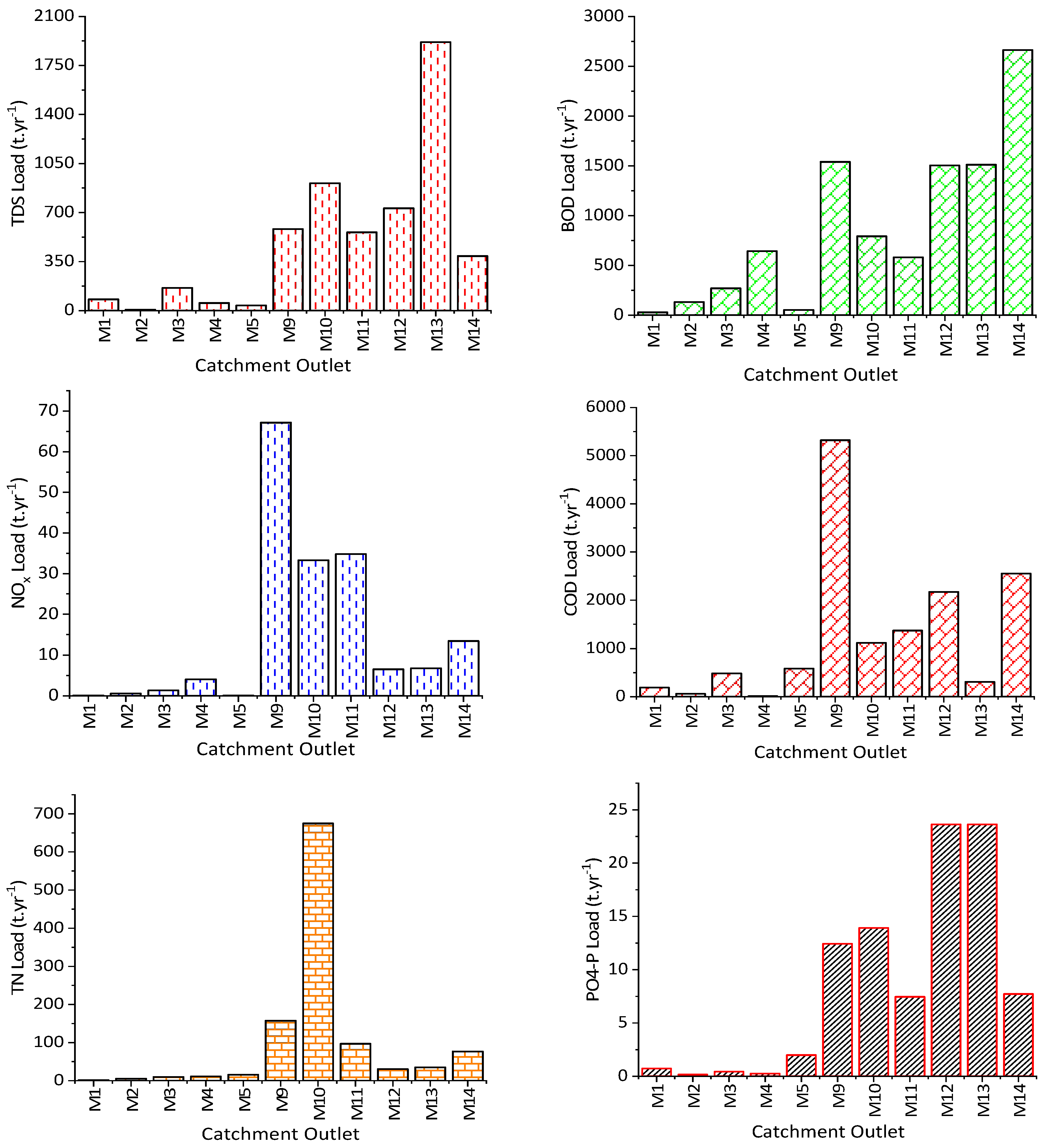
Pa = parameters; differential load = incremental load of the downstream station relative to the upstream station/s; NO_x ^* = reported as NO₃+NO₂; ^† deficit (sink).

), we found that the prevalence of differential uncharacterized nonpoint source load at the middle and downstream segment of the LAR with highest calculated differential load were BOD, COD, and TDS, which had shown highest loads at segment outlets M9, M10, M12, M13, and M14, and the influence of uncharacterized nonpoint sources were found to be significantly high (Figure 5). The areas were dominated by urban set-ups (industrial with both large and small scale), residential settlement (usually informal), and agricultural (predominantly small scale) land uses. The organic pollution contribution from the nonpoint sources prevailed in the study area where the maximum calculated differential BOD load was observed at M9 with 1833.2 t/yr, where the station is located downstream of two highly polluted but large streams that make a confluence. On the other hand, the maximum COD differential load from the nonpoint source was observed at the same station with a calculated load of 5588.7 t/yr contributed by the subcatchment having an area of 826.419 ha, followed by M13, M12, and M10, which had contributed an annual load of 3217.2 t, 2306.9 t, and 1859.55 t, respectively. Similarly, high BOD depletion was observed at downstream stations M10 (1867.49 t/yr), M11 (738.49 t/yr), and M14 (1007.76 t/yr), where the impacts of nonpoint sources were assumed to be insignificant, showing that the river is going through a high rate of recovery, possibly due to morphometric effects and the improved self-purification capacity of the river [55].

High PO₄-P differential load was calculated at most downstream stations characterized by small-scale urban agricultural activities prevailing at M12 (23.63 t/yr), followed by M10 (12.92 t/yr) and M9 (12.42 t/yr). Besides, the area is characterized by a large number of small-scale industries, dumping sites for informal solid waste including bio-waste, wastewater treatment plant effluent, and animal remains. On the other hand, from Table 6, it can be seen that high differential TN load from uncharacterized nonpoint source was calculated at monitoring stations M9 (157.2 t/yr), M10 (674.79 t/yr), and M11 (97.02 t/yr), whereas stations M4, M12, and M13 were identified as areas with TN sink. COD, BOD, TDS, and TN were found to be dominant nonpoint source load contributions and were found in large quantities prevailing in the middle and downstream segments, indicating the increased impact of washouts from agricultural and urban land uses. The CMB analysis in LAR revealed that most of the organic waste load were concentrated at the middle segment of the river, whereas the sink for these pollutants was found far downstream. The CMB analysis in LAR also showed that NO_x, TN, and BOD had sinks at most of the LAR monitoring stations calculated at outlets. Stations M9–M14 are the recognized sink areas for organic pollutants and nutrients located in the middle and downstream segments of LAR. A similar finding was reported by Elósegui et al. [56], where most of the nutrient load in river Agüera in Northern Spain was retained in the middle of the river. The station M11 is a place where the organic pollutants are highly degraded and hence the area was identified as a major nutrient sink. It is a place where a public protected park (Biheretsige Park) is located, which could reduce the impact of nonpoint source load contributions. Relative to the downstream and middle catchments, the upstream segments have low nonpoint source load contributions, where a similar result was also found by Jain et.al. [33] on Hindon River, India. This could be due to relatively low flow, less anthropogenic influence in the area, and the presence of buffer zones such as grass strips and urban forests.

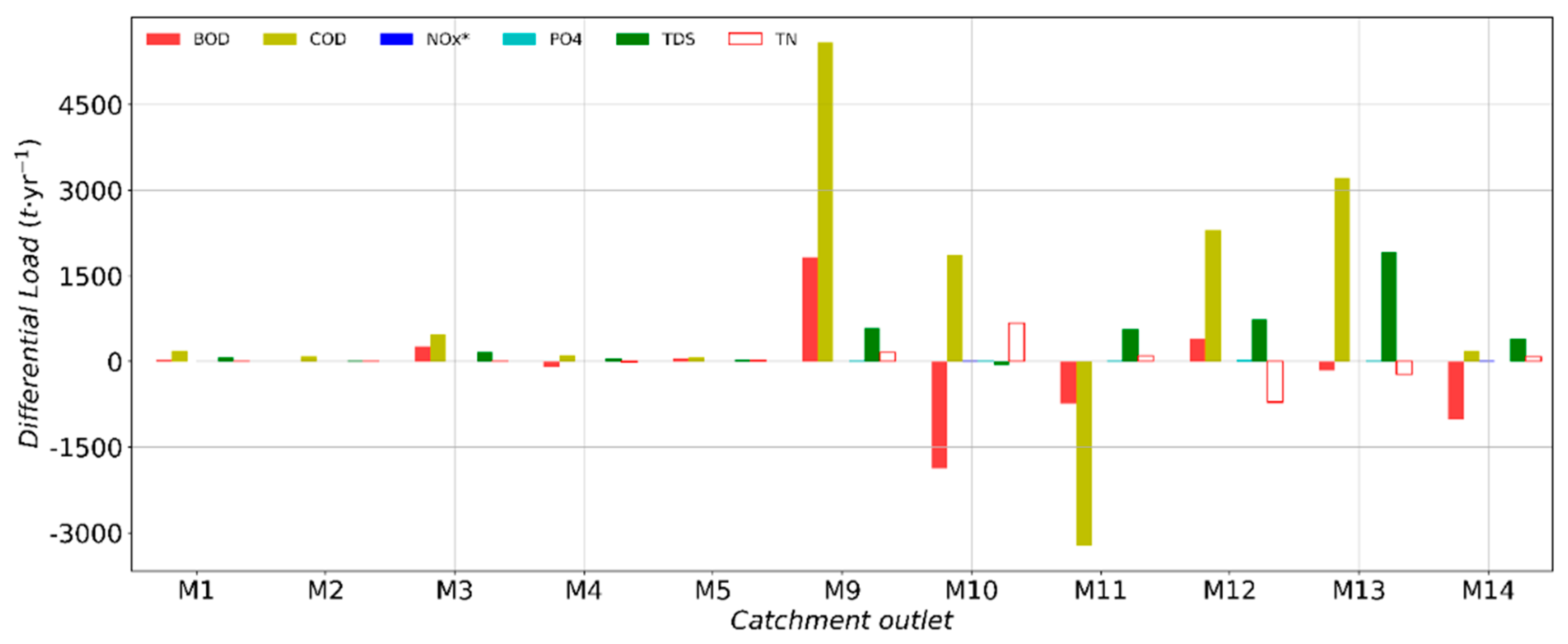
From the CMB analysis (Figure 6), it can be seen that most of the constituents in the upstream section of the LAR (M1–M5) had minimum differential load, showing reduced impact of nonpoint source pollution. Conversely, differential loads of BOD, TN, and NO_x have shown most of the sinks were observed at the middle and downstream segment of LAR, where riversides are protected by grasses and plants, predominantly at M10 and M11. Maximum loads of nutrients, such as TN, NO_x, and PO4-P, were recorded at M10, which was also identified as a major sink for BOD. Similarly, M14 was found as an area where both TN and NO_x have shown a positive differential load. The station is found downstream of the discharge point of wastewater treatment plant effluent and is also characterized by small-scale urban agriculture.

3.4. Integration of CMB-PLOAD and Uncharacterized Nonpoint Source Load

Loads calculated at selected LAR subcatchment outlets (monitoring stations) by CMB were used for PLOAD calibration and the selected ECf for LAR was used as an initial estimation for calibration. During the calibration of PLOAD in Excel Solver, the ECf were used as independent variables and the ranges were constraints by setting the upper and lower bounds of the ECf based on the literature for optimization. At the initial stage of calibration and preoptimization, the total percentage error between the model-predicted and measured load at all monitoring stations for COD, BOD, TDS, NO_X, PO₄-P, and TN were 3680.6%, 2965.64%, 767.97%, 446.8%, 750.40%, and 899.36% respectively. After the optimization of the ECf in Solver, the average percentage relative error dropped to 12.16%, 3.98%, 0.53%, 26.86%, 8.9%, and 29.22%, respectively. On the other hand, the sum of errors in COD was found to be higher than BOD, which resulted in a total sum of error at 3680.6% preoptimization, where much was attributed by station M5, at which point the PLOAD underestimated both constituents at the station.

The PLOAD prediction for TDS was relatively accurate, where the total relative error at all monitoring stations before optimization was found to be 767.97%, which sharply dropped to 0.53% after optimization. Unlike other parameters, the PLOAD model has overestimated the TDS load in the upstream section of the LAR (M1–M5, and M9), whereas the model underestimated the PO₄-P load in LAR at the downstream segment of the river. High total errors were recorded at smaller catchments of LAR than the bigger catchments, and Zinabu et.al. [1] also came up with a similar finding in Kombolcha catchment, Ethiopia. From the optimized ECf, we found that urban and agricultural land use ECf varies greatly with varying urban land-use types and has shown a significant variation spatially. The water body land-use showed minimum change over the loading of constituents across the monitoring stations, which could be due to less area coverage in the watershed.

The PLOAD was rerun using the median and mean value of the optimized and calibrated ECf. Though the median ECf gave minimum total percentage error relative to the mean value, high variation in the ranges of the ECf made the load vary greatly, and hence the loads calculated by both mean and median ECf were not acceptable. The optimized ECf values revealed that the use of average and median value resulted in an underestimation of pollutant load at some catchment outlets, whereas overestimation on others. Thus, the use of area-specific ECf was relatively acceptable and was found effective in better estimation of pollutant loads in LAR. The study conducted by Shrestha et al. [11] also recommended the use of area-specific, and development of local, ECf for effective pollutant load calculations. The optimized values can then be interpreted well for LAR and used for the management of the nonpoint source pollution load in the catchment. Similarly, the PLOAD was validated for a different data set without change in the optimized export coefficient and the error calculated from the model was acceptable enough for further interpretation. Accordingly, the percentage error between the PLOAD predicted and measured values for COD, BOD, TDS, NO_x, PO₄-P, and TN during validation were found to be 16.41%, 7.06%, 1.77%, 13.23%, 5.4%, and 18.83%, respectively.

The calibrated pollutant ECfs showed that the urban land uses had significantly varying export coefficients. Accordingly, the pollutant loading rate for urban land use ranged from 42.1–2083 kg/ha/yr, 63.3–2012 kg/ha/yr, and 0.49–1.6 kg/ha/yr for COD, TDS, and PO₄-P, respectively, varying with the subtype of urban land use (such as residential, commercial, industrial) and location. The urban land uses dominated by residential settlements and industries do have high loading rates, whereas other urban land uses have relatively lesser rates. Similarly, the urban land use pollutant ECf for BOD and NO_x also vary greatly, ranging from 120–1950.55 kg/ha/yr and 0.1–47.32 kg/ha/yr respectively. The high variation in ECf spatially is due to the high difference in the impact of nonpoint sources among various urban land uses. The upstream urban land uses have less pollutant loading than the middle and downstream catchments (

Table 7. Uncharacterized nonpoint source load in LAR by integrating CMB and PLOAD, t/y.

R ‡	TDS	BOD	COD	PO4-P	TN	NOX
M1	80.77	27.82	189.96	0.72	1.768	0.102
M2	6.56	132.09 †	62.432	0.155 †	5.391	0.572 †
M3	162.18	269.69	482.89	0.431	10.217	1.352
M4	54.055	644.28 †	14.31	0.243	11.232 †	4.063
M5	36.76	51.91	585.64	1.993	15.913	0.083
M9	581.95	1540.12	5319.119	12.428	157.242	67.168 †
M10	910.12 †	792.220	1119.375	13.921	674.791	33.304
M11	558.85	581.51 †	1367.92 †	7.460	97.018	34.825 †
M12	730.78	1504.80 †	2170.24	23.627	30.462 †	6.529 †
M13	1916.16	1511.69 †	308.91	23.628	35.453 †	6.791 †
M14	389.72	2664.75 †	2551.43	7.717†	76.825	13.454

^† Loads where the deficit was calculated by CMB analysis but PLOAD estimated the value from nearby subcatchment EC_f; ^‡ catchment outlet where PLOAD was calibrated, and hence represents catchment nonpoint source load contribution.

). The agricultural land use for all the constituents was sensitive in controlling the impact of the pollutants load on the LAR. Though the contribution of agricultural land for nonpoint COD load was quite constant with a range of 79.64–81 kg/ha/yr, an appreciable magnitude of ECf for TDS with 76.4–2005 kg/ha/yr would suggest that the agricultural land use varies spatially in contributing the TDS loading rate. Similarly, PO₄-P, NO_x, and BOD have an annual loading rate of 7.72–8.1 kg/ha, 0.1–30.16 kg/ha, and 60.25–60.8 kg/ha/yr from the agricultural land use.

4. Conclusions

In this study, conjunctive application of chemical mass balance and watershed model, PLOAD, was used to estimate the nonpoint source load in the data-scarce Little Akaki River, Ethiopia, which was found effective. The approach proved to be more efficient in the study area, which ultimately focused on the determination of organic pollutants and nutrient loads based on a continuously monitored water quality data in the river. The following major conclusions were drawn from the research findings.

• The impact of nonpoint sources in the upstream segment of the LAR catchment was relatively less than the downstream and middle segments, primarily due to the reduced impacts of unrecognized point sources, less urban settlements, better land-use protection and management. Moreover, lesser flow rate in the upper segment of the river could be playing a critical role for the lower diffuse source load in the area.
• The integration of CMB and catchment nonpoint source pollution models such as PLOAD could be an effective and alternative pollutant load estimation approach in data scarce areas.
• The nonpoint source pollutant load was found to be very high in areas where urban land uses prevail, followed by agricultural and barren land uses, indicating the nonpoint source pollution management focus areas. Mitigation measures involving these land uses is recommended.
• Area-specific (local) pollutant export coefficients were found to be more effective and accurate load estimation approach than the use of mean and median export coefficients, which ultimately give a lower error during pollutants load calculation. Despite higher accuracy of CMB for the estimation of differential uncharacterized nonpoint source load estimation, integrating with a simple watershed model was found to be a good alternative for a more accurate representation of the diffuse source load.
• Under- and overestimation of the PLOAD for pollutant load estimation was observed at some catchment outlets, which when integrated with CMB analysis gave a promising result. But adaptation of global export coefficient to the local condition with different hydro-climatic setup is the limitation of the integral modeling approach.
• The pollutant and nutrient export coefficients developed in LAR catchment could be transferred to other catchment elsewhere in the country for similar application for preliminary nonpoint source pollutant load management. The accuracy and effectiveness of the CMB for nonpoint source load estimation highly depends on a number of factors, such as frequency of data collection, distance between the monitoring stations, and identification of the major point sources to the river.

It could be concluded that the integral application of chemical mass balance and watershed models such as PLOAD could be a better option for the estimation of nonpoint source pollutant loads in areas with few monitored water quality data. Future studies incorporating the vast and long-term monitoring program at larger catchment scale would be helpful for better pollution load management in the river.

References

1. Zinabu, E.; van der Kwast, J.; Kelderman, P.; Irvine, K. Estimating Total Nitrogen and Phosphorus Losses in a Data-Poor Ethiopian Catchment. J. Environ. Qual. 2017, 46, 1519–1527. [Google Scholar] [CrossRef] [PubMed]
2. Gurung, D.P.; Githinji, L.J.; Ankumah, R.O. Assessing the Nitrogen and Phosphorus Loading in the Alabama (USA) River Basin Using PLOAD Model. Air Soil Water Res. 2013, 6, 23–36. [Google Scholar] [CrossRef]
3. Ongley, E.D.; Xiaolan, Z.; Tao, Y. Current status of agricultural and rural non-point source Pollution assessment in China. Environ. Pollut. 2018, 158, 1159–1168. [Google Scholar] [CrossRef] [PubMed]
4. Chen, D.; Dahlgren, R.A.; Lu, J. A modified load apportionment model for identifying point and diffuse source nutrient inputs to rivers from stream monitoring data. J. Hydrol. 2013, 501, 25–34. [Google Scholar] [CrossRef] [Green Version]
5. Hao, G.; Li, J.; Li, S.; Li, K.; Zhang, Z.; Li, H. Quantitative assessment of non-point source pollution load of PN/PP based on RUSLE model: A case study in Beiluo River Basin in China. Environ. Sci. Pollut. Res. 2020, 27, 33975–33989. [Google Scholar] [CrossRef]
6. Huiliang, W.; Zening, W.; Caihong, H.; Xinzhong, D. Water and nonpoint source pollution estimation in the watershed with limited data availability based on hydrological simulation and regression model. Environ. Sci. Pollut. Res. 2015. [Google Scholar] [CrossRef]
7. Liu, Y.; Li, H.; Cui, G.; Cao, Y. Water quality attribution and simulation of non-point source pollution load flux in the Hulan River basin. Sci. Rep. 2020, 10, 1–15. [Google Scholar] [CrossRef] [Green Version]
8. Wu, L.; Liu, X.; Ma, X. Spatio-temporal variation of erosion-type non-point source pollution in a small watershed of hilly and gully region, Chinese Loess Plateau. Environ. Sci. Pollut. Res. 2016, 23, 10957–10967. [Google Scholar] [CrossRef]
9. Wu, L.; Gao, J.; Ma, X.; Li, D. Application of modified export coefficient method on the load estimation of non-point source nitrogen and phosphorus pollution of soil and water loss in semiarid regions. Environ. Sci. Pollut. Res. 2015, 22, 10647–10660. [Google Scholar] [CrossRef]
10. Chen, Y.; Zang, L.; Shen, G.; Liu, M.; Du, W.; Fei, J.; Yang, L. Resolution of the Ongoing Challenge of Estimating Nonpoint Source Neonicotinoid Pollution in the Yangtze River Basin Using a Modified Mass Balance Approach. Environ. Sci. Technol. 2019, 53, 2539–2548. [Google Scholar] [CrossRef]
11. Shrestha, S.; Kazama, F.; Newham, L.T.H.; Babel, M.S.; Clemente, R.S.; Ishidaira, H.; Nishida, K.; Sakamoto, Y. Catchment scale modelling of point source and non-point source pollution loads using pollutant export coefficients determined from long-term in-stream monitoring data. J. Hydro-Environ. Res. 2008, 2, 134–147. [Google Scholar] [CrossRef]
12. Waseem, M.; Koegst, T.; Tränckner, J. Groundwater Contribution to Surface Water Contamination in a North German Low Land Catchment with Intensive Agricultural Land Use. J. Water Resour. Prot. 2018, 10, 231–250. [Google Scholar] [CrossRef] [Green Version]
13. Waseem, M.; Schilling, J.; Kachholz, F.; Tränckner, J. Improved representation of flow and water quality in a North-eastern German lowland catchment by combining low-frequency monitored data with hydrological modelling. Sustainability 2020, 12, 4812. [Google Scholar] [CrossRef]
14. Raj, P.; Lee, S.; Lee, Y.; Kanel, S.R.; Pelletier, G.J. Application of automated QUAL2Kw for water quality modeling and management in the Bagmati River, Nepal. Ecol. Modell. 2007, 202, 503–517. [Google Scholar] [CrossRef]
15. Berndtsson, R. Transport and sedimentation of pollutants in a river reach: A chemical mass balance approach. Water Resour. Res. 1990, 26, 1549–1558. [Google Scholar] [CrossRef]
16. Morris, A.W.; Allen, J.I.; Howland, R.J.M.; Wood, R.G. The Estuary Plume Zone: Source or Sink for Land-derived Nutrient Discharges? Estuar. Coast. Shelf Sci. 1995, 40, 387–402. [Google Scholar] [CrossRef]
17. Jain, C.K.; Bhatia, K.K.S.; Seth, S.M. Assessment of point and non-point sources of pollution using a chemical mass balance approach. Hydrol. Sci. J. 1998, 43, 379–390. [Google Scholar] [CrossRef]
18. Dolan, D.M.; El-Sharawi, A.H. Inferences about Point Source Loadings from Upstream/Downstream River Monitoring Data. Environ. Monit. Assess. 1989, 12, 343–357. [Google Scholar] [CrossRef]
19. Feyisa, G.L.; Dons, K.; Meilby, H. Landscape and Urban Planning Efficiency of parks in mitigating urban heat island effect: An example from Addis Ababa. Landsc. Urban Plan. 2014, 123, 87–95. [Google Scholar] [CrossRef]
20. Arsiso, B.K.; Tsidu, G.M.; Stoffberg, G.H.; Tadesse, T. Climate Risk Management Climate change and population growth impacts on surface water supply and demand of Addis Ababa, Ethiopia. Clim. Risk Manag. J. 2017, 18, 21–33. [Google Scholar] [CrossRef]
21. Yohannes, H.; Elias, E. Contamination of Rivers and Water Reservoirs in and Around Addis Ababa City and Actions to Combat It. Environ. Pollut. Clim. Chang. 2017, 1, 1–12. [Google Scholar] [CrossRef]
22. Aschale, M.; Sileshi, Y.; Kelly-Quinn, M.; Hailu, D. Evaluation of potentially toxic element pollution in the benthic sediments of the water bodies of the city of Addis Ababa, Ethiopia. J. Environ. Chem. Eng. 2016, 4, 4173–4183. [Google Scholar] [CrossRef]
23. Beyene, A.; Addis, T.; Kifle, D.; Legesse, W.; Kloos, H.; Triest, L. Comparative study of diatoms and macroinvertebrates as indicators of severe water pollution: Case study of the Kebena and Akaki rivers in Addis Ababa, Ethiopia. Ecol. Indic. 2009, 9, 381–392. [Google Scholar] [CrossRef]
24. APHA; AWWA; WEF. Standard Methods for the Examination of Water and Wastewater. In American Public Health Association (APHA); American Public Health Association: Washington, DC, USA, 2017. [Google Scholar]
25. Lai, Y.C.; Yang, C.P.; Hsieh, C.Y.; Wu, C.Y.; Kao, C.M. Evaluation of non-point source pollution and river water quality using a multimedia two-model system. J. Hydrol. 2011, 409, 583–595. [Google Scholar] [CrossRef]
26. Han, L.; Huo, F.; Sun, J. Method for calculating non-point source pollution distribution in plain rivers. Water Sci. Eng. 2011, 4, 83–91. [Google Scholar] [CrossRef]
27. Falconer, L.; Telfer, T.C.; Ross, L.G. Modelling seasonal nutrient inputs from non-point sources across large catchments of importance to aquaculture. Aquaculture 2018, 495, 682–692. [Google Scholar] [CrossRef] [Green Version]
28. Jamwal, P.; Mittal, A.K.; Mouchel, J.M. Point and non-point microbial source pollution: A case study of Delhi. Phys. Chem. Earth 2011, 36, 490–499. [Google Scholar] [CrossRef]
29. Walker, W.W. Simplified Procedures for Eutrophication Assessment and Prediction: User Manual; U.S. Army Corps of Engineers: Washington, DC, USA, 1999. [Google Scholar]
30. Amaya, F.L.; Gonzales, T.A.; Hernandez, E.C.; Luzano, E.V.; Mercado, N.P. Estimating Point and Non-Point Sources of Pollution in Biñan River Basin, the Philippines. In Proceedings of the International Conference on Environmental Science and Development-ICESD, Hong Kong, China, 5–7 January 2012; Volume 1, pp. 233–238. [Google Scholar]
31. Xin, X.; Yin, W.; Li, K. Estimation of non-point source pollution loads with flux method in Danjiangkou Reservoir area, China. Water Sci. Eng. 2017, 10, 134–142. [Google Scholar] [CrossRef]
32. Albek, E. Estimation of point and diffuse contamination loads to streams by non-parametric regression analysis of monitoring data. Water. Air. Soil Pollut. 2003, 147, 229–243. [Google Scholar] [CrossRef]
33. Jain, C.K.; Singhal, D.C.; Sharma, M.K. Estimating nutrient loadings using chemical mass balance approach. Environ. Monit. Assess. 2007, 134, 385–396. [Google Scholar] [CrossRef]
34. Sekhar, M.C.; Sreenivasulu, D. Modelling Nutrients Contributed by Overland Flow from the Krishna River Basin. In Proceedings of the Diffuse Pollution Conference: Water Resouces Management, Dublin, Ireland, 17–21 August 2003; pp. 20–23. [Google Scholar]
35. Li, Z.; Luo, C.; Jiang, K.; Wan, R.; Li, H. Comprehensive Performance Evaluation for Hydrological and Nutrients Simulation Using the Hydrological Simulation Program—Fortran in a Mesoscale Monsoon Watershed, China. Int. J. Environ. Res. Public Health 2017, 14, 1599. [Google Scholar] [CrossRef] [PubMed] [Green Version]
36. Wang, X.; Yang, H.; Cai, Y.; Yu, C.; Yue, W. Identification of optimal strategies for agricultural nonpoint source management in Ulansuhai Nur watershed of Inner Mongolia, China. Stoch. Environ. Res. Risk Assess. 2016, 30, 137–153. [Google Scholar] [CrossRef]
37. Kipyego, S.; Ouma, Y. Analysis of Nonpoint Source Pollution Loading on Water Quality in an Urban- Rural River Catchment Using GIS-PLOAD Model: Case Study of Sosiani River. Civ. Environ. Res. 2018, 10, 70–84. [Google Scholar]
38. Santhi, C.; Arnold, J.G.; Williams, J.R.; Dugas, W.A.; Srinivasan, R.; Hauck, L.M. Validation of the SWAT Model on a Large River Basin with Point and Nonpoint Sources. J. Am. Water Resour. Assoc. 2001, 37, 1169–1188. [Google Scholar] [CrossRef]
39. Shen, Z.; Hong, Q.; Chu, Z.; Gong, Y. A framework for priority non-point source area identification and load estimation integrated with APPI and PLOAD model in Fujiang Watershed, China. Agric. Water Manag. 2011, 98, 977–989. [Google Scholar] [CrossRef]
40. USEPA PLOAD: An ArcView GIS Tool to Calculate Nonpoint Sources of Pollution in Watershed and Stormwater Projects- version 3.0; United States Environmental Protection Agency: Washington, DC, USA, 2001.
41. Lin, J.P. “Review of Published Export Coefficient and Event Mean Concentration (EMC) Data” WRAP Technical Notes Collection (ERDC TN-WRAP-04-3); U.S. Army Engineer Research and Development Center: Vicksburg, MS, USA, 2004. [Google Scholar]
42. Ma, X.; Li, Y.; Zhang, M.; Zheng, F.; Du, S. Assessment and analysis of non-point source nitrogen and phosphorus loads in the Three Gorges Reservoir Area of Hubei Province, China. Sci. Total Environ. 2011, 412–413, 154–161. [Google Scholar] [CrossRef]
43. Jeje, Y. Export coefficients for total phosphorus, total nitrogen and total suspended solids in the southern Alberta region: A review of literature. In Alberta; Alberta Environment: Calgary, AB, Canada, 2016; pp. 1–22. [Google Scholar]
44. Chang, N.; Chen, H.W.; Jeng, K.S.; Ning, S.K.; Lee, C.S. Evaluation of non-point source loads in the reservoir watershed using the GIS/GPS/RS information technologies and numerical models. Water Int. 2001, 26, 239–251. [Google Scholar] [CrossRef]
45. Alexander, R.B.; Elliott, A.H.; Shankar, U.; McBride, G.B. Estimating the sources and transport of nutrients in the Waikato River Basin, New Zealand. Water Resour. Res. 2002, 38, 4-1–4-23. [Google Scholar] [CrossRef]
46. Fleifle, A.; Saavedra, O.; Yoshimura, C.; Elzeir, M.; Tawfik, A. Optimization of integrated water quality management for agricultural efficiency and environmental conservation. Environ. Sci. Pollut. Res. 2014, 21, 8095–8111. [Google Scholar] [CrossRef]
47. Povilaitis, A. Source apportionment and retention of nutrients and organic matter in the merkys river basin in southern Lithuania. J. Environ. Eng. Landsc. Manag. 2010, 16, 195–204. [Google Scholar] [CrossRef]
48. Haith, D.A.; Mandel, R.; Wu, R.S. GWLF Generalized Watershed Loading Functions Version 2.0 User’s Manua; Department of Agricultural and Biological Engineering, Cornell University: Ithaca, NY, USA, 1992. [Google Scholar]
49. Wali, U.G.; Nhapi, I.; Ngombwa, A.; Banadda, N.; Nsengimana, H.; Kimwaga, R.J.; Nansubuga, I. Modelling of Nonpoint Source Pollution in Akagera Transboundary River in Rwanda. Open Environ. Eng. J. 2011, 4, 124–132. [Google Scholar] [CrossRef] [Green Version]
50. Moriasi, D.N.; Arnold, J.G.; Van Liew, M.W.; Bingner, R.L.; Harmel, R.D.; Veith, T.L. Modeling Evaluation Guidelines for Systemiatic Quantification of Accuracy in Watershed Simulations. Am. Soc. Agric. Biol. Eng. 2007, 50, 885–900. [Google Scholar] [CrossRef]
51. Abbaspour, K.C.; Rouholahnejad, E.; Vaghefi, S.; Srinivasan, R.; Yang, H.; Kløve, B. A continental-scale hydrology and water quality model for Europe: Calibration and uncertainty of a high-resolution large-scale SWAT model. J. Hydrol. 2015, 524, 733–752. [Google Scholar] [CrossRef] [Green Version]
52. Rostamian, R.; Jaleh, A.; Afyuni, M.; Mousavi, S.F.; Heidarpour, M.; Jalalian, A.; Abbaspour, K.C. Application of a SWAT model for estimating runoff and sediment in two mountainous basins in central Iran. Hydrol. Sci. J. 2008, 53, 977–988. [Google Scholar] [CrossRef]
53. Shawul, A.A.; Chakma, S.; Melesse, A.M. The response of water balance components to land cover change based on hydrologic modeling and partial least squares regression (PLSR) analysis in the Upper Awash Basin. J. Hydrol. Reg. Stud. 2019, 26, 100640. [Google Scholar] [CrossRef]
54. Jain, C.K. Application of chemical mass balance approach to determine nutrient loading. Hydrol. Sci. 2000, 45, 577–588. [Google Scholar] [CrossRef]
55. Setiawan, A.D.; Widyastuti, M.; Hadi, M.P. Water quality modeling for pollutant carrying capacity assessment using Qual2Kw in bedog river. Indones. J. Geogr. 2018, 50, 49–56. [Google Scholar] [CrossRef] [Green Version]
56. Elósegui, A.; Arana, X.; Basaguren, A.; Pozo, J. Self-purification processes along a medium-sized stream. Environ. Manag. 1995, 19, 931–939. [Google Scholar] [CrossRef]
Figure 1. The Little Akaki River (LAR) water quality monitoring stations and point source locations.
Sustainability 12 07084 g001
Figure 2. Land use map of the study area.
Sustainability 12 07084 g002
Figure 3. Soil and water assessment tool (SWAT) simulation for flow at Big Akaki River (BAR) (calibration and validation).
Sustainability 12 07084 g003
Figure 4. Plot of SWAT simulated versus observed flow in BAR (a) calibration and (b) validation (black diagonal line is a one to one (equality) line).
Sustainability 12 07084 g004
Figure 5. Nonpoint source pollutant loads at selected catchment outlets of LAR (t/yr).
Sustainability 12 07084 g005
Figure 6. Differential pollutants load calculated at selected monitoring stations in LAR (t/yr).
Sustainability 12 07084 g006