Article

Protected Landscapes in Spain: Reasons for Protection and Sustainability of Conservation Management

by
Nicolas Marine
1,*,
Cecilia Arnaiz-Schmitz
2,*,
Cristina Herrero-Jáuregui
2,
Manuel Rodrigo de la O Cabrera
1,
David Escudero
1 and
María F. Schmitz
2
1
Department of Architectural Composition, Escuela Tecnica Superior de Arquitectura de Madrid, Universidad Politécnica de Madrid, 28040 Madrid, Spain
2
Department of Biodiversity, Ecology and Evolution, Complutense University of Madrid, 28040 Madrid, Spain
*
Authors to whom correspondence should be addressed.
Sustainability 2020, 12(17), 6913; https://doi.org/10.3390/su12176913
Submission received: 10 July 2020 / Revised: 15 August 2020 / Accepted: 23 August 2020 / Published: 25 August 2020

Abstract

:
Landscape conservation efforts in many European countries focus on cultural landscapes, which are part of the cultural identity of people, have a great heritage significance, improve the living standards of local populations and provide valuable cultural biodiversity. However, despite a wide arrange of protective measures, the management of preserved areas is seldom effective for the protection of cultural landscapes. Through a multi-approach analysis, we characterise the main heritage attributes of 17 Protected Landscapes in Spain and assess their management effectiveness by quantifying the evolution of the spatial pattern inside and outside protected landscapes. Our method has proven useful to quantitatively describe the spatial-temporal patterns of change of the protected and unprotected landscapes studied. We highlight the following results: (i) the concepts of uniqueness and naturalness are not appropriate to preserve cultural landscapes; (ii) the land protection approach currently adopted is not useful for the protection of cultural landscapes, particularly of the most rural ones; (iii) the landscapes studied with greater rural features can be considered as “paper parks”. We recommend that different protection measures focused on the needs and desires of the rural population are taken into account in order to protect cultural landscapes that are shaped by traditional rural activities.

1. Introduction

As a consequence of relevant international initiatives concerning landscape protection, at the end of the 20th century [1,2,3] the effectiveness of already implemented legal mechanisms for land management has been questioned [4,5]. The assumption that landscape conservation policies are a multi-sector concern essential for sustainable land development calls for an adjustment of existing legal frameworks to more contemporary criteria. Thus, several authors have analysed the capability of existing legislation for the protection of landscape values and for granting collaborative and integrated land management [6,7,8,9]. Conservation efforts in many European countries have therefore focused on landscapes depending on human intervention. These cultural landscapes, which are part of the cultural identity of people, have a great heritage significance, improve the living standards of local populations and provide valuable cultural biodiversity [10,11,12,13].
The International Union for Conservation of Nature (IUCN) [14] has recognized the value of working landscapes as protected areas, naming them “Protected Landscapes “, the only one of the six IUCN protected area management categories based on the interaction between people and nature (Category V of IUCN Protected Areas). The exceptional natural and cultural values of these landscapes have encouraged measures for their protection. These types of landscape are a relevant reference for the implementation of a sustainable lifestyle [15]. Due to their origin in the long-term coevolution of natural and anthropogenic factors, Protected Landscapes have a strong correspondence with the UNESCO definition of Cultural Landscapes [16,17]. Furthermore, IUCN’s Category V set a clear precedent [18] for the protection of Cultural Landscapes and many studies equate both categories for a possible joint implementation [19,20,21]. However, the disparity between landscapes that are part of Category V is remarkable and Protected Landscapes throughout Europe show many differences not only their natural, cultural, and social characteristics but also in the legislation and the reasons considered for protection.
In Spain, the legal figure of Protected Landscape was incorporated in 1989, as part of a comprehensive natural conservation law. The inclusion of protected landscapes in the Spanish territorial regulation involved a legal novelty of some importance, since, among the different protection categories established, Protected Landscapes were the only ones that lacked some precedents. The Law of 1989 defined Protected Landscapes as “those specific places of the natural environments that deserve special protection because of their cultural and aesthetic values” (art. 17). Both in definition and aim, this figure has a clear precedent in IUCN’s Category V, whose definition precedes that of Spanish Protected Landscapes by one year [21,22]. For the first time in Spain, cultural and perceptual values were recognized as key components of landscapes and protected within an environmental legal framework [23]. Furthermore, the recognition of this figure anticipated concepts that would later be brought to the Spanish debate on landscape protection and management policies under the influence of UNESCO and the Council of Europe [24,25] (see Table 1 for a comparison of the definition of Spanish protected landscapes with that of other international protection categories of similar scope). Thus, Spanish Protected Landscapes are connected in concept with several international proposals for sustainable management focused on the relationship between humans and their environment, which has led to important initiatives, such as the Spanish National Plan for Cultural Landscapes (PNPC) [26]. The ratification in 2007 of the European Landscape Convention promoted the promulgation of a revised law that adjusted Spanish Protected Landscapes to the definition given by the Council of Europe [27]. As a consequence, this legal protection figure has not only embraced and adapted the ideas and concepts from various international organisms but also has enough longevity to verify its long term effectiveness.
In spite of all these protection measures, and although they supply considerable amounts of ecosystem services [28,29], several authors have demonstrated that too often, the management of protected areas is not effective for the protection of cultural landscapes [30,31]. To the ubiquitous tendency of rural-urban migration and rural abandonment, strict legal requirements and the lack of encouragement of rural activities do not favour the maintenance of the societal structure that gave rise to the landscapes that are to be preserved. Thus, very often those cultural landscapes subject of conservation, even if protected and in many cases because of mistaken protection measures, evolve to other types of landscapes, dominated by unmanaged forests [32,33]. Following on our previous works, we hypothesise that in Spain the Protected Landscapes category does not have effective management for the protection of cultural rural landscapes.
On this basis, we focus here on empirically identifying the main characteristics of Protected Landscapes in Spain, as well as analysing their management effectiveness. The present paper is proposed with the following objectives: (i) to quantify the evolution of the spatial pattern inside and outside protected landscapes and detect the main indicators of landscape change; (ii) to identify types of protected landscapes according to their land-use composition, spatial structure and intensity of change; (iii) to characterise the different types of protected landscapes according to their heritage attributes; iv) to evaluate the management effectiveness and sustainability of the Protected Landscape category to preserve cultural landscapes.

2. Material and Methods

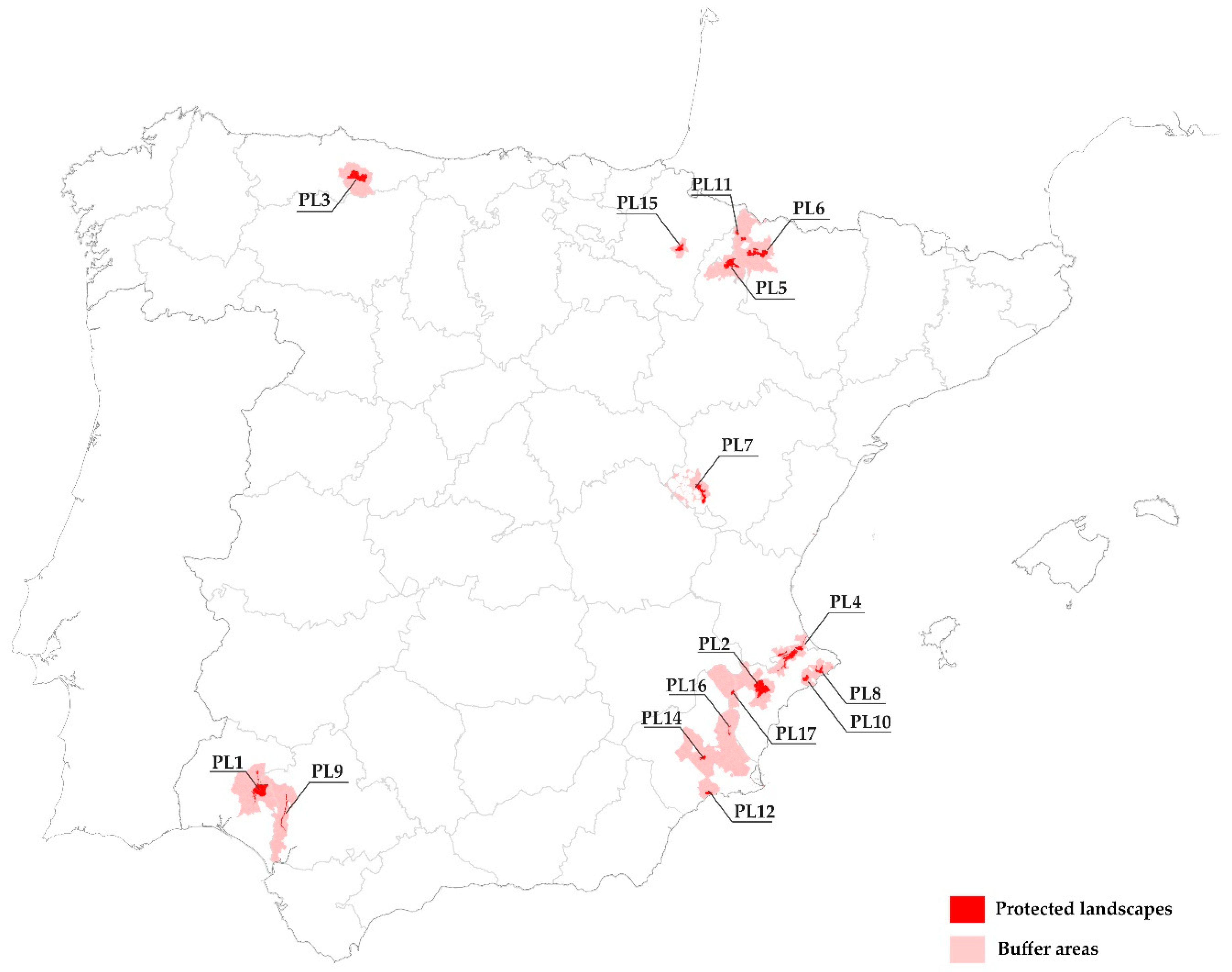
2.1. Sample Study. Selection of Protected Landscapes

For the declaration of a territory as a protected landscape, the Spanish legislation requires compliance with three basic aspects: (1) the conservation of unique values; (2) the preservation of the harmonious interaction between culture and nature, and (3) the defence of traditional practices. The conceptual differences in the application of this figure are manifested in a wide variety of legal protection instruments. Since 1989 and to date, different Spanish regions have declared a total of 58 Protected Landscapes. Of them, 31 are in the Iberian Peninsula and 27 in the Canary Islands.
Generally, these protected landscapes are representative of historical relationships between societies and their environment, although certain regions have opted for the sole conservation of fauna and flora. Notably, there has also been a tendency to protect special river sections [23]. The extent of protected areas is a less consistent factor and varies greatly from one landscape to another. Thus, an average range between 300 and 6000 ha can be determined, although several landscapes have an area greater than 10,000 ha. Another factor of difference between Spanish regions is that some (such as Cataluña, Castilla y León or Madrid) do not have any protected area under this category.
The current list of Protected Landscapes constitutes a representative sample of the multiple types of cultural landscapes in Spain. The criteria followed by the Spanish Administration for the protection of these landscapes are based on their typological representativeness and geographic diversity. In accordance with these criteria, for this study, we selected a sample of 17 peninsular landscapes illustrative of this great variety. The selected places are located in different regions of Spain (Figure 1) and therefore have different natural and cultural characteristics (Table 2). These areas have been declared protected in different periods of time (Table 2). The selected landscapes also comply with the requirement of having a continuous protection area. The Spanish legislation is unclear in this regard and some landscapes are composed of a collection of discontinuous areas. In this case, the only selected landscape with a divided area included in the sample is the “Paisaje protegido de las Fozes de Fago y Biniés” [34]. This landscape comprises two close areas very similar in size and shape. Considering management schemes, the Spanish legislation regulates the declaration of protected landscapes and the different regions develop the appropriate management plans to achieve their conservation goals. None of the selected landscapes is under other types of national or international protection.

2.2. Methods

We focused on spatial-temporal changes in the landscapes studied and considered the dynamics of their structural characteristics four times over 22 years (1990, 2000, 2006, 2012). A general outline of the steps followed in the methodological approach is shown in Figure 2.

2.2.1. Data Collection and Analyses

Landscape structure was quantified by means of landscape and patch metrics (LMs), whose values are effective indicators of spatial patterns [35,36]. To calculate them: (i) we used CORINE Land Cover Maps of the years 1990, 2000, 2006 and 2012, considering seven land use-land cover types (LULCs) based on the reclassification of the Corine land cover classes into more meaningful and representative categories. The LULCs used were: forest systems, shrublands, dehesas (open woodlands used as pastures), agricultural systems, urban systems, rocky areas and wetlands/water bodies; (ii) we selected sixteen spatially explicit and non-redundant LMs, characterized by their easy interpretation and their ability to quantify landscape patterns [30,37]; (iii) we used Fragstats 4.2 [35] for the calculation of the selected LMs [38] (see the method of calculation and a brief description of each LMS in Appendix A): Shannon’s diversity index (SHDI) quantifies landscape diversity and it is a good indicator of landscape heterogeneity; Shannon’s evenness index, Simpson’s evenness index and Modified Simpson’s evenness index (SHEI, SIEI and MSIEI, respectively) measure the distribution of areas among patch types. As such, evenness is contrary to dominance; Patch richness density (PRD) measures the number of patch types present; Number of patches (NP) is a simple measure of the extent of subdivision of the patch type; Total edge and Edge density (TE and ED, respectively) inform about the amount of edge created by the patches present in the landscape. NP and edge metrics, together with Landscape Division index (DIVISION) and Splitting index (SPLIT), measure the degree of landscape fragmentation; Core Area index (CAI) is a relative index that quantifies the percentage of core area in a patch. This index could serve as an effective fragmentation index for a particular patch type. Landscape Contagion index (CONTAG) measures both the spatial dispersion of a patch type and the intermixing of units of different patch types at landscape level; Contiguity index (CONTIG) assesses spatial patch contiguity or connectedness; Patch Cohesion index (COHESION) calculates the physical connectedness of the corresponding patch types in an area and Euclidean nearest neighbour distance (ENN) describes the degree of spatial isolation of patches and, therefore, the degree of landscape connectivity; Largest patch index (LPI), measures the size of patches and the amount of edge created by these patches and represents an indirect measure of landscape homogeneity. We generated raster maps of the set of LMs by means of a round moving window with a radius of 100 m and then extracted a mean value of each metric for each of the 17 protected cultural landscapes selected.
We used the same procedure to characterise a buffer around each protected landscape whose area corresponds to that of the administrative divisions of the municipalities included in the respective studied landscape. This design allowed us to quantify inside and outside processes between protected and unprotected landscapes. To quantify the structure and dynamics of cultural landscapes, we elaborated a quantitative data matrix consisting of two sub-matrices describing, respectively, the characteristics of the 17 protected landscapes studied and their surrounding territories in the time span studied, using the 23 selected variables (7 LULCs and 16 LMs). This data matrix was analysed using successive applications of Principal Component Analyses (PCAs), in a multi-approach considering the inside and outside design.

2.2.2. Quantifying the Evolution of Protected and Unprotected Cultural Landscapes

With the collected data, we analysed landscape changes over time taking into account the initial and final periods registered (1990 and 2012): (i) inside and outside the protected cultural landscapes, and (ii) only within protected landscapes. We performed two PCAs at two spatial-temporal scales, respectively. The first PCA was calculated on the whole data matrix and the second one only on the protected landscape submatrix. These two PCAs allowed us to project the distribution of the protected landscape-unprotected matrix systems and inside protected landscapes on their respective ordination planes. Their dimensions represent, according to the factor loadings of the descriptive variables, the two main tendencies of variation of the landscapes and their changes over time.

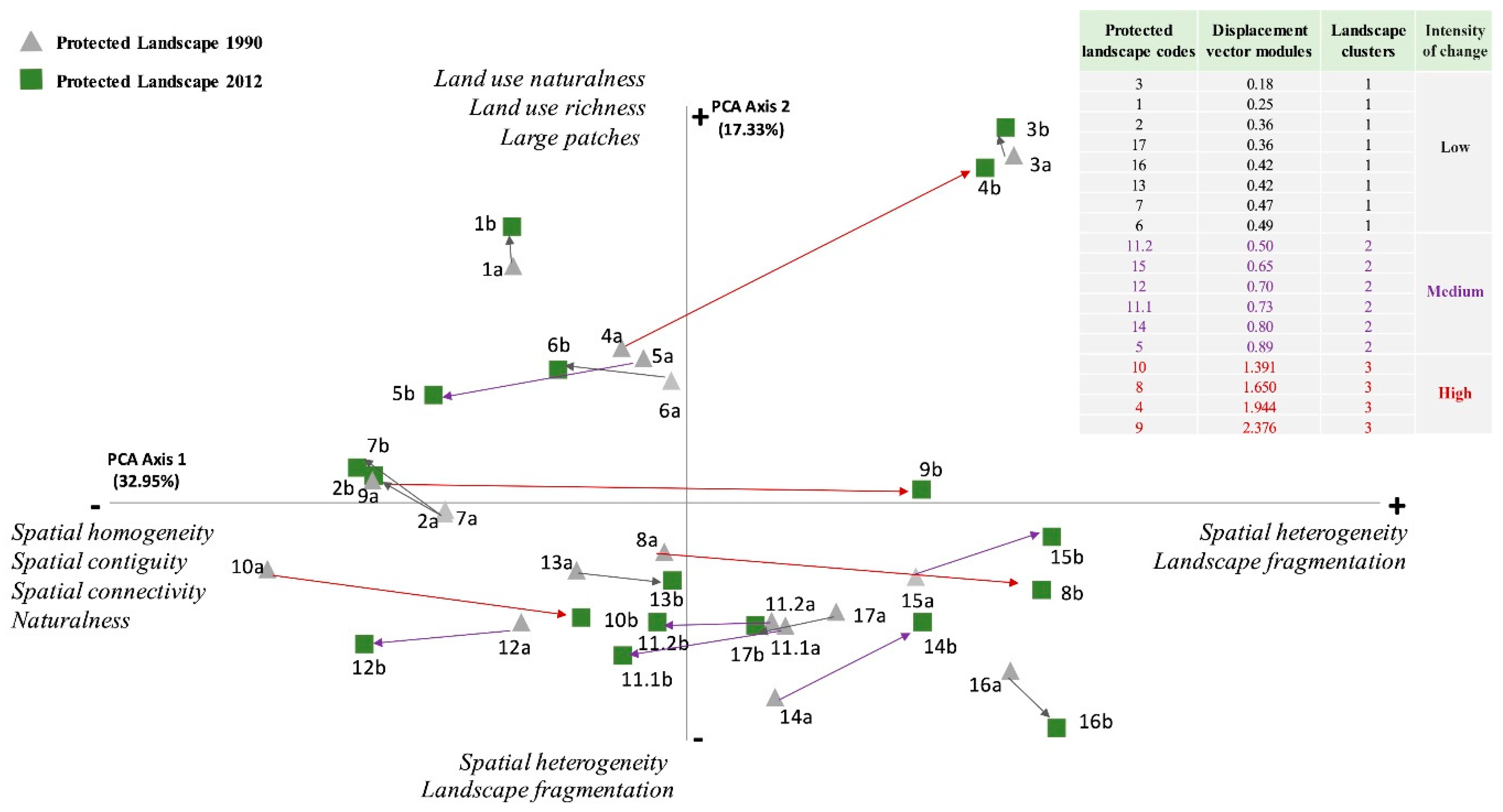
2.2.3. Calculating the Intensity of Change inside Protected Areas for Landscape Characterisation

We analysed the trajectories of the changes occurred inside the protected landscapes, as well as their intensity, by calculating the displacement vectors,   D V i of the coordinates of each landscape on the PCA plane from time t1 (1990) to time t2 (2012) (1). The direction of D V i on the ordination plane indicates the tendency of landscape change and their module values the intensity of temporal change.
D V i = ( x t 2 i x t 1 i ) 2 + ( y t 2 i y t 1 i ) 2 + ( n t 2 i n t 1 1 ) 2
We identified three types of landscapes according to the magnitude of their change, based on the value of the modules of their displacement vectors, by means of the equal intervals method: highly dynamic landscapes (high intensity of change), landscapes of moderate change (medium intensity of change) and landscapes without significant changes (low intensity of change).
We subsequently proceeded to confront the landscape types obtained with the heritage values detected in each of the landscapes. For this purpose, we adapted a list of attributes already tested as a viable method to characterise Spanish cultural landscapes [25]. As a basis for the characterisation, we used the original declaration documents which describe the main historical and geographical attributes of each of the landscapes. The final result is a list divided into two categories: human activities and historical remains. In turn, these are formed by several features described in Table 3. It is significant to note that the list complies with the requirements for cultural characterisation recommended by researchers attached to UNESCO [39], by ICOMOS [40] and by the Spanish PNPC [26]. These features were used as external descriptors describing the three landscape types previously obtained. The procedure was performed using a mean comparison test that allowed us to characterise a qualitative variable through quantitative variables. Therefore, Fisher’s F-test (k > 2) was used to determine the statistical significance of the variables (heritage attributes) in the landscape types (landscape clusters obtained). The more the mean of a variable in a group is significantly different from the mean of that variable in the whole group, the stronger the link between the characterising quantitative variable and the qualitative category [41].
The landscape group corresponding to high intensity of change was analysed by means of a third PCA considering its detailed structure variation over time (complete temporal trajectory: 1990, 2000, 2006 and 2012). The date of the declaration of protected landscapes and / or that of their specific management plans were taken into account as external categorical variables of the calculated spatial-temporal patterns.

3. Results

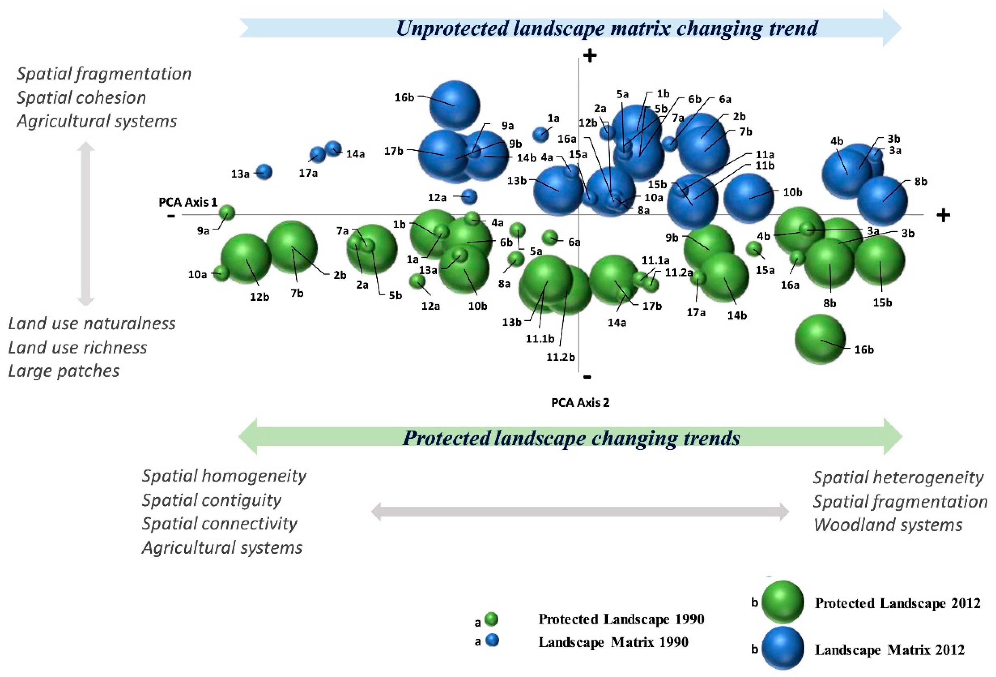
3.1. Landscape Dynamics inside and outside Protection

The analysis performed on the entire landscape data matrix, composed by the selected protected landscapes and their surrounding unprotected areas (PCA1; see Figure 2), allowed us to identify the trajectories of landscape change throughout the study period (Figure 3). The PCA plane reveals the main variation tendencies of landscape composition and structure, according to the loadings of the landscapes’ variables. PCA axis 1 (explained variance: 29.72%) expresses the dynamics of the landscape in the studied time spam. The indicators of the landscape change (variables with the highest factor loadings) have allowed us to identify the more significant variation in its structure and composition (Table 4a). Thus, the surrounding territorial matrix has undergone a transformation process towards greater spatial heterogeneity linked to land use richness and fragmentation (LMs characterising the positive end of axis 1: SHDI, DIVISION, SHEI, MSIEI, SIEI, PRD, ED and SPLIT; see Appendix A and Table 4a), in which the dominant land uses are those related to the development of woodland systems, mainly composed of forests and dehesas. On this PCA axis 1, the dynamics of protected landscapes have followed in part (n = 9) the same spatial heterogeneity trend as that of the landscape matrices in which they are immersed, and in part (n = 8) the opposite tendency (negative end of axis 1), towards spatial homogenization, land use spatial contiguity and connectivity (landscape structure indicators: LPI, CONTAG, ENN, CAI, COHESION; see Appendix A and Table 4a) and agricultural systems as prevalent land uses (Table 4a; Figure 3).
It is remarkable that PCA axis 2 (explained variance: 21%) shows a noticeable difference between the protected landscape and the surrounding landscape matrix, in each case (Figure 3). The indicators of this disparity express a greater naturalness in protected landscapes than in unprotected lands, with large patches of different natural systems (variables with higher factor loadings at the negative end of axis 2: PRD, LPI; forest systems, shrublands and rocky areas; Table 4a; Figure 3). The positive end of axis 2 is related to unprotected agricultural landscapes characterised by areas with a high number of patches and spatial cohesion, indicating a greater degree of aggregation among fragments in agricultural landscapes than in woodland systems (detected through landscape indicators by PCA axis 1; landscape structure indicators: NP, TE, COHESION; Appendix A and Table 4a; Figure 3).

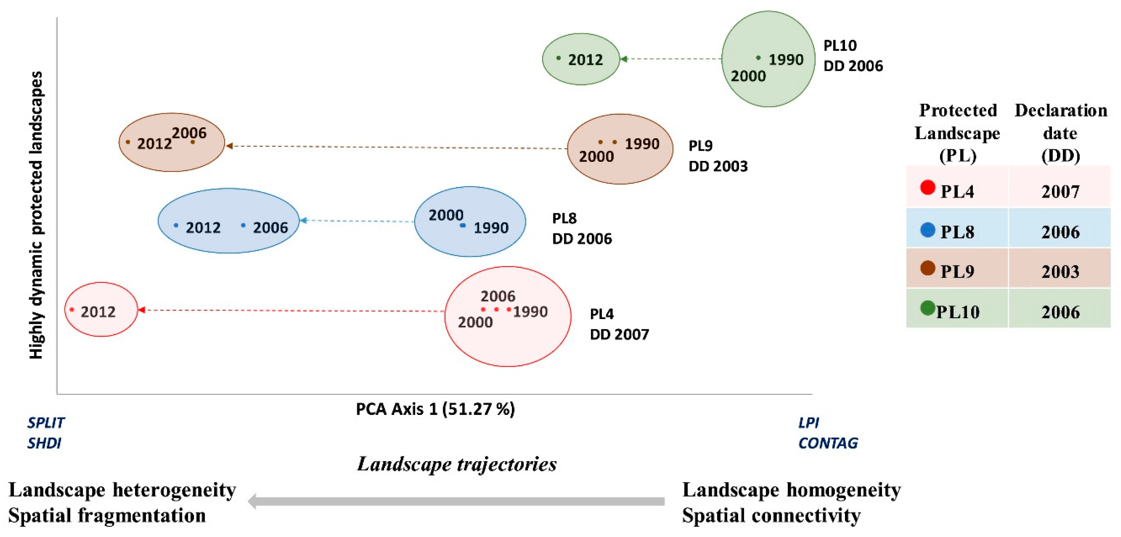
3.2. Spatial-Temporal Variation inside Protected Landscapes

The PCA carried out on the sub-matrix collecting the temporal data of the protected landscapes allowed us to identify that the two main axes of the analysis explained the same variation in their composition and structure, highlighting changes over time in their heterogeneous-homogeneous spatial patterns and land-use fragmentation processes, as indicated by the variables with the greatest loadings at the ends of each axis (Figure 4; Table 4b). Thus, at the negative end of axis 1 (explained variance: 32.95%), landscape homogeneity is expressed by means of LPI and CAI, and metrics such as ENN, CONTAG, COHESION and CONTIG are mainly linked to low fragmentation, contiguity of land uses and landscape connectivity. Spatial contiguity of land uses and landscape connectivity are indicated by COHESION and CONTIG. Forests and shrublands land uses with high loadings at this end of PCA axis 1, are representative of the naturalness of the landscape. In contrast, the positive end of axis 1 is characterised by indicators of spatial heterogeneity (SIEI, SHEI, MSIEI, SHDI) and landscape fragmentation (DIVISION, ED, SPLIT). PCA 2 (explained variance: 17.33%) discriminates among the most natural protected landscapes from those mainly characterised by spatial heterogeneity and land-use fragmentation. In this axis 2 (negative end), PRD and LPI metrics are the indicators of landscapes with large patches of natural land uses (rocky areas and wetlands/water bodies) and SPLIT, DIVISION, TE and NP indices describe processes of landscape heterogeneity and fragmentation (positive end).
The calculation on the PCA plane of the displacement vectors between the coordinates of protected landscapes from the initial to the final times studied (1990 and 2012, respectively) enabled us to determine the direction (spatial homogeneity versus spatial heterogeneity) and magnitude (modules of displacement vectors) of landscape changes. The vector modules indicate high variability in the intensity of landscape changes. We identified three types of landscapes with different intensity of change by classifying the displacement vectors into three clusters according to the magnitude of their modules: (i) Landscape cluster 1. Composed of 8 of the 17 protected landscapes studied and characterised by a low intensity of change; value of the vector modules = 0 ≥ D V i     < 0.5. The direction and sense of the change trajectories of this group of vectors are variable; (ii) Landscape cluster 2. Composed of 5 protected landscapes with a medium intensity of change; value of the vector modules = 0.5 ≤     D V i     < 1. Temporal landscape trajectories do not follow a particular pattern; (iii) Landscape cluster 3. Composed of 4 protected landscapes of high intensity of change; value of the vector modules = 1 ≤   D V i   . The landscape change trend is directed towards spatial heterogeneity and fragmentation (Figure 4).
These landscape clusters were statistically characterised by the heritage features described in Table 3 (human activities and historical remains), which prevailed in the territories studied at the time of their declaration as protected landscapes. Significant statistical attributes considered for protection were those related to cultural heritage, rurality and traditional land uses and practices, as well as landscape features, indicators of aesthetic quality (Table 5). Protected landscapes with the lowest dynamics of change in the period studied (Landscape cluster 1; low intensity of change) were characterised by attributes related to agrarian systems and an economy oriented to local production. Landscapes characterised by their aesthetic or symbolic values showed a medium rate of change (Landscape cluster 2; medium intensity of change). Rural landscapes with traditional forms of land use, agricultural practices and water management have experienced a high intensity of change since their declaration as protected landscapes (Landscape cluster 3).
The PCA performed on the data matrix containing descriptive variables of the 4 protected landscapes identified as highly dynamic (Landscape cluster 3), is shown in Figure 5. The LMs selected for this analysis were some of the ones that were detected as the most representative indicators of the changes in the landscape structure in the previous PCAs (NP, COHESION, ENN, PRD, CAI, SHDI, CONTAG, SPLIT and LPI). Since, at this scale, the variance explained by the PCA axis 1 was very high (51.27%), only the variation expressed by this first axis has been considered. LMs characterising the ends of the axis (greater factor loadings; Table 4c) express the spatial-temporal variation of these changing landscapes from homogeneity and connectivity (as indicated by LPI and CONTAG metrics) to heterogeneity and fragmentation (processes represented by the land metrics SHDI and SPLIT). Likewise, the analysis of the complete temporal trajectory registered has allowed us to identify that the transformation of these territories towards fragmentation and spatial heterogeneity has been significantly greater since their declaration as Protected Landscapes (see Figure 5, Declaration date). In Figure 5 the length of the arrows indicates the magnitude of the landscape change.

4. Discussion

The essential rationale for this paper is to know the main reasons behind the decision to preserve landscapes and formally designate them under the protected landscape category. The design inside and outside the protection limits has been successful in achieving the established objectives and has allowed us to evaluate the management effectiveness of the protected landscapes studied. This inside-out approach to estimating protected area effectiveness is a frequently adopted strategy that provides useful insights and knowledge about processes related to land protection [12,32,33,42,43,44,45,46]. The multi-approach analysis performed considering the inside and outside design and the landscape metrics calculated [38,47] has provided a useful methodological tool and an effective set of spatial indicators to quantitatively describe the spatial-temporal patterns of change of the protected and unprotected landscapes studied. Furthermore, this approach has allowed us to verify how the dynamics of the landscape inside and outside the protection boundaries has had an evident effect on landscape configuration.
Comparing variations in landscape composition and structure inside versus outside protection shows a great difference between protected and unprotected land (detected by PCA axis 2; Figure 3). The landscape indicators identified evidence the naturalness of protected landscapes, mainly composed of large patches of different forest systems, shrublands and rocky areas, which characterise and differentiate them from the matrix of mainly agricultural unprotected landscapes in which they are immersed. The great disparity observed between protected landscapes and their surrounding unprotected land matrices indicates the trend towards the protection of certain peculiar features highlighted in human-dominated landscapes, mainly linked to landscape naturalness and uniqueness. Protection of naturalness has traditionally been a central objective of conservation efforts [48,49]. However, in cultural landscapes with a long history of human-maintained systems, it is controversial to consider naturalness as a point of reference to design conservation and management plans [32]. Especially for the Protected Landscape category, whose main reason is to prevent the loss of landscapes, that represent a valuable natural and cultural heritage [50].
The detected indicators of the landscape spatial-temporal change also express a remarkable transformation process, especially pronounced in unprotected landscapes (Figure 3; PCA axis 1). This transformation reflects higher land-use fragmentation and spatial heterogeneity, associated with the disruption of landscape connectivity and to the development of woodland systems as a consequence of the abandonment of agricultural land uses. Modified landscapes are often presented as patches of native vegetation within a matrix of different characteristics [51]. Spatial fragmentation is a complex and progressive process that leads to the division of continuous habitat into smaller and more isolated patches that are separated by dissimilar land matrices [52,53]. Worldwide, habitat loss and fragmentation are some of the main drivers of change in landscape structure and in the intensity of ecological interactions and are linked to environmental exploitation by humans [54]. However, in cultural landscapes habitat fragmentation means the transformation and disconnection of multifunctional agricultural landscapes, which are abandoned or intensified, affecting their functionality and ecological integrity [55]. The loss of traditional land uses and agricultural economic base has resulted in the observed fragmentation of agricultural lands and the consequent change of character and loss of visual quality [56].
The establishment of protected areas has been the primary management measure to preserve landscapes from this abandonment process [57]. Nevertheless, a significant number of the Protected Landscapes studied have followed a trend of transforming their spatial patterns through fragmentation, breaking contiguous landscapes (Figure 3; PCA axis 1). Thus, the spatial-temporal analysis of the studied protected landscapes show the same dynamic described above of landscape transformation towards spatial fragmentation and, as a by-product, spatial heterogeneity (Figure 4). Fragmentation resulting from habitat loss inevitably leads to greater heterogeneity, directly through a change of state or fragment conversion, or indirectly through edge effects [58]. Along with this process, alterations in spatial connectivity occur, since as fragmentation increases, connectivity values become critical [59]. This has happened with particular intensity in most rural landscapes. Indeed, the results obtained through vector analysis highlight that while some of the landscapes studied remain relatively unchanged or little altered, traditional rural landscapes experienced a great intensity of change and that their marked fragmentation process coincides in each case with the date of their designation as a Protected Landscape (Landscape cluster 3; Figure 4; Figure 5, respectively).
The literature on the role of protected areas in the conservation of cultural landscapes and the effectiveness of their management is abundant. These aspects, however, are especially critical in human-dominated landscapes since their protection has traditionally also involved their abandonment and the loss of their heritage values [10,60]. Similar results have been found in Central Spain, where relict hedgerow networks follow similar trajectories of abandonment inside and outside protected areas, revealing a lack of effectiveness of conservation measures [33,46]. In the same region, Sarmiento-Mateos et al [31] found incoherencies in the regulatory schemes of a protected area network, that inhibit rural inhabitants to continue with their traditional activities causing negative consequences for the cultural landscape whose protection is intended.
In summary, there has been a tendency to protect unique landscapes of a more natural character, which contradicts the initial objective of the Protected Landscape category. Furthermore, this category was conceived as part of what IUCN calls a “protected area system” [61]. Protected Landscapes are a very specific category and are not supposed to be declared as isolated entities. Instead, they should be part of a broader conservation plan that includes other categories. In fact, the Natural Heritage and Biodiversity Law (42/2007), that defined Protected landscapes, was modified partially in 2015 by another law [62]. Although it did not change their definition, it introduced the concept of Green Infrastructure and its necessity of being considered jointly with existing protected areas. This follows an initiative for establishing protected landscape networks similar to other European actions [63,64].
And so, Protected Landscapes in Spain have proven to be particularly inefficient to protect rural landscapes. Although the important role assigned to protected areas has driven their establishment, the focus of their conservation and management plans, which favours the constant change of protected sites, makes them vulnerable to accusations of not achieving some of the conservation objectives. Reliance on regulatory schemes and their effective application in landscape management is difficult and too often fails [65], which triggers that some protected areas to be just “paper parks“ [66,67]—protected only in name.

5. Conclusions

The methodological approach developed has provided us with an effective set of indicators to quantitatively describe and compare the spatial-temporal patterns of change in the protected and unprotected landscapes studied. The marked disparity observed inside and outside protection highlighted the trend towards protecting the naturalness and uniqueness of the landscape. The quantitative indicators identified also detected a general transformation of the landscape towards spatial heterogeneity and land-use fragmentation, mainly related to the abandonment of agricultural land uses and the expansion of woodlands. This transformation process has been especially pronounced in unprotected landscapes, although it has also occurred in a large part of protected landscapes.
The analyses performed considering the trajectories of the spatial-temporal changes of Spanish Protected Landscapes allowed us to recognise types of landscapes, quantify their intensity of change and identify the different heritage characteristics considered as base values for their protection. Furthermore, through this procedure, we were able to detect the protected landscapes that had maintained their characteristics over time and those that had undergone an accelerated change. In this regard, it is noteworthy that after the declaration of protection, traditional rural landscapes experienced a great intensity of change towards non-rurality characteristics, as opposed to the primary objective of the category of Protected Landscape. Thus, in line with our starting hypothesis, the designation of the Protected Landscape category has not been an effective tool to protect rural landscapes.
The applied methodological design has proven to be useful in providing empirical information on the main reasons taken into account to protect the cultural landscape under the category of Protected Landscape, as well as on the effectiveness of its management guidelines. From the results obtained, we state the need to develop protection schemes in the Spanish legislation focused on traditional knowledge and on the essential requirements of rural populations to effectively protect the valuable heritage of cultural landscapes, mainly shaped by traditional rural activities.

Author Contributions

Conceptualization, N.M., C.A.-S., M.R.d.l.O.C. and D.E.; methodology, N.M., C.A.-S., M.F.S. and C.H.-J.; software, N.M. and C.A.-S.; formal analysis, C.A.-S.; investigation, N.M., C.A.-S., M.F.S. and C.H.-J.; writing—original draft preparation, N.M., C.A.-S., M.F.S. and C.H.-J.; writing—review and editing, N.M., C.A.-S., M.F.S., C.H.-J., M.R.d.l.O.C. and D.E.; funding acquisition, M.R.d.l.O.C. and D.E. All authors have read and agreed to the published version of the manuscript.

Funding

This research was funded by the project LABPA-CM: Contemporary Criteria, Methods and Techniques for Landscape Knowledge and Conservation (H2019/HUM-5692), funded by the European Social Fund and the Madrid regional government.

Acknowledgments

The authors would like to thank Guillermo Sotelo Santos and Paula Nogueira Losada for its valuable help in data gathering.

Conflicts of Interest

The authors declare no conflict of interest. The funders had no role in the design of the study; in the collection, analyses, or interpretation of data; in the writing of the manuscript; or in the decision to publish the results.

Appendix A

Table A1. Landscape metrics and patch metrics used to calculate landscape spatial patterns [35]. A brief description of the metrics used is provided, as well as their calculation methods and ranges of variation.
Landscape MetricsFormulaRange and Description
Shannon’s Evenness Index S H E I = i = 1 m ( P i ln P i ) ln m
Pi = proportion of the landscape occupied by patch type (i)
m = number of patch types (i) present in the
landscape, excluding the landscape border if present
SHEI > 0, without limit
It is expressed so that an even distribution of area among patch types results in maximum evenness. As such, evenness is the complement of dominance.
Shannon’s Diversity Index S H D I = i = 1 m ( P i ln P i )
Pi = proportion of the landscape occupied by patch type (i)
SHDI > 0, without limit
SHDI = 0 when the landscape contains only 1 patch (i.e., no diversity). SHDI increases as the number of different patch types (i.e., patch richness, PR) increases and/or the proportional distribution of area among patch types becomes more equitable.
Patch richness density P R D = m A ( 10000 ) ( 100 )
m = number of patch types present in the landscape
a = Total landscape area
PRD > 0, without limit.
Number of different patch types present within the landscape boundary.
Splitting index S P L I T = A 2 j = 1 n a i j 2
aij = area (m2) of patch ij.
A = total landscape area (m2)
1 ≤ SPLIT ≤ number of cells in the landscape squared.
Increases as the landscape is increasingly subdivided into smaller patches and achieves its maximum value when the landscape is maximally subdivided; that is, when every cell is a separate patch.
Euclidean nearest neighbour distanceENN = hij
hij = distance (m) from patch ij to nearest neighbouring patch of
the same type (class), based on patch edge-to-edge distance, computed from cell center to cell center
ENN > 0, without limit.
Distance (m) to the nearest neighbouring patch of the same type, based on the shortest edge-to-edge distance. It has been used extensively to quantify patch isolation
Largest Patch Index L P I =   M a x   ( a ) A   × ( 100 )
aij = area (m2) of patch ij.
A = total landscape area (m2)
0 < LPI < 100
Percentage of the total landscape comprising the largest patch
Contagion Index C O N T A G = [ 1 + i = 1 m k = 1 m [ ( P i ) ] [ g i k k = 1 m g i k ] [ ln ( P i ) [ g i k k = 1 m g i k ] ] 2 ln m ] ( 100 )
Pi = proportion of the landscape occupied by patch type i.gik number of adjacencies (joins) between pixels of patch types (classes) i and k based on the double-count method.
m = number of patch types (classes) present in the landscape.
0 < CONTAG ≤ 100
It approaches 0 when the patch types are maximally disaggregated and interspersed. CONTAG = 100 when all patch types are maximally aggregated; i.e., when the landscape consists of a single patch.
Patch Cohesion Index C O H E S I O N = [ 1 j = 1 n p i j j = 1 n p i j a i j ] [ 1 1 A ] 1 ( 100 )
pij = perimeter of patch ij in terms of number of cell surfaces
aij = area of patch ij in terms of number of cells
A = total number of cells in the landscape
0 ≤ COHESION < 100
It measures the physical connectedness of the corresponding patch type
Core Area Index C A I = a i j c a i j
aijc = core area (m2) of patch ij based on specified edge depths (m).
aij = area (m2) of patch ij.
0 ≤ CAI < 100
CAI approaches 100 when the patch, because of size, shape, and edge width, contains mostly core area. A patch with no core area has the highest edge effect and consequently, the ecological processes of the patch may not function properly
Contiguity Index C O N T I G = [ r = 1 s c i j r a i j ] 1 v     1
cijr = contiguity value for pixel r in patch ij.
v = sum of the values in a 3-by-3 cell template (13 in this case).
aij = area of patch ij in terms of number of cells
0 ≤ CONTIG ≤ 1
This index assesses the spatial connectedness, or contiguity. Equals 0 for a one-pixel patch and increases to a limit of 1 as patch contiguity, or connectedness, increases. Thus, large contiguous patches result in larger contiguity index values
Edge density E D = E A ( 10000 )
E = total length (m) of edge in landscape.
A = total landscape area (m2).
ED ≥ 0, without limit.
ED = 0 when there is no edge in the landscape; that is, when the entire landscape and landscape border, if present, consists of a single patch.
Modified Simpson’s Evenness Index M S I E I = ln i = 1 m p i 2 ln m
Pi = proportion of the landscape occupied by patch type (class) i.
m = number of patch types (classes) present in the landscape.
0 ≤ MSIEI ≤ 1
MSIDI = 0 when the landscape contains only 1 patch (i.e., no diversity) and approaches 0 as the distribution of areas among the different patch types becomes increasingly uneven (i.e., dominated by one type). MSIDI = 1 when the distribution of areas among patch types is perfectly even.
Simpson’s Evenness Index S I E I = 1 i = 1 m p i 2 1 ( 1 m )
Pi = proportion of the landscape occupied by patch type (class) i.
m = number of patch types (classes) present in the landscape, excluding the landscape border if present.
0 ≤ SIEI ≤ 1
SIDI = 0 when the landscape contains only 1 patch (i.e., no diversity) and approaches 0 as the distribution of areas among the different patch types becomes increasingly uneven (i.e., dominated by one type). SIDI = 1 when the distribution of areas among patch types is perfectly even.
Total edge T E = E
E = total length (m) of edge in landscape.
TE ≥ 0, without limit.
TE = 0 when there is no edge in the landscape; that is, when the entire landscape consists of a single patch.
Number of patches N P = n i
ni = number of patches in the landscape of patch type i.
NP ≥ 1, without limit.
NP = 1 when the landscape contains only 1 patch of the corresponding patch type. It is a simple measure of the extent of subdivision or fragmentation of the patch type.
Landscape Division Index D I V I S I O N = [ 1 i = 1 m j = 1 m ( a i j A ) 2 ]
aij = area (m2) of patch ij.
A = total landscape area (m2).
0 ≤ DIVISION < 1
DIVISION = 0 when the landscape consists of a single patch. DIVISION achieves its maximum value when the landscape is maximally subdivided. It is similar to a diversity index

References

  1. IUCN. Guidelines for Protected Area Management Categories; IUCN: Gland, Switzerland; Cambridge, UK, 1994. [Google Scholar]
  2. UNESCO. Report of the World Heritage Committee Sixteenth Session (Santa Fe, United States of America, 7–14 December 1992). In Convention Concerning the Protection of the World Cultural and Natural Heritage; UNESCO: Santa Fe, NM, USA, 1992. [Google Scholar]
  3. Council of Europe. European Landscape Convention; Council of Europe Publishing Division: Strasbourg, France, 2000. [Google Scholar]
  4. Mitchell, N.; Rössler, M.; Tricaud, P. World Heritage Cultural Landscapes: A Handbook for Conservation and Management; UNESCO: Paris, France, 2009. [Google Scholar]
  5. De Montis, A. Impacts of the European Landscape Convention on national planning systems: A comparative investigation of six case studies. Landsc. Urban Plan. 2014, 124, 53–65. [Google Scholar] [CrossRef]
  6. García-Martín, M.; Bieling, C.; Hart, A.; Plieninger, T. Integrated landscape initiatives in Europe: Multi-sector collaboration in multi-functional landscapes. Land Use Policy 2016, 58, 43–53. [Google Scholar] [CrossRef] [Green Version]
  7. Janssen, J. Sustainable development and protected landscapes: The case of The Netherlands. Int. J. Sustain. Dev. World Ecol. 2009, 16, 37–47. [Google Scholar] [CrossRef] [Green Version]
  8. Nogueira Terra, T.; Ferreira dos Santos, R.; Cortijo Costa, D. Land use changes in protected areas and their future: The legal effectiveness of landscape protection. Land Use Policy 2014, 38, 378–387. [Google Scholar] [CrossRef]
  9. De Montis, A. Measuring the performance of planning: The conformance of Italian landscape planning practices with the European Landscape Convention. Eur. Plan. Stud. 2016, 24, 1727–1745. [Google Scholar] [CrossRef]
  10. Agnoletti, M. Rural landscape, nature conservation and culture: Some notes on research trends and management approaches from a (southern) European perspective. Landsc. Urban Plan. 2014, 126, 66–73. [Google Scholar] [CrossRef]
  11. Marull, J.; Tello, E.; Fullana, N.; Murray, I.; Jover, G.; Font, C.; Coll, F.; Domene, E.; Leoni, V.; Decolli, T. Long-term bio-cultural heritage: Exploring the intermediate disturbance hypothesis in agro-ecological landscapes (Mallorca, c. 1850–2012). Biodivers. Conserv. 2015, 24, 3217–3251. [Google Scholar] [CrossRef] [Green Version]
  12. Vlami, V.; Kokkoris, I.P.; Zogaris, S.; Cartalis, C.; Kehayias, G.; Dimopoulos, P. Cultural landscapes and attributes of “culturalness” in protected areas: An exploratory assessment in Greece. Sci. Total. Environ. 2017, 595, 229–243. [Google Scholar] [CrossRef]
  13. Campedelli, T.; Calvi, G.; Rossi, P.; Trisorio, A.; Florenzano, G.T. The role of biodiversity data in High Nature Value Farmland areas identification process: A case study in Mediterranean agrosystems. J. Nat. Conserv. 2018, 46, 66–78. [Google Scholar] [CrossRef]
  14. Janssen, J.; Knippenberg, L.W.J. From landscape preservation to landscape governance: European experiences with sustainable development of protected landscapes. In Studies on Environmental and Applied Geomorphology; Piacentini, T., Miccadei, E., Eds.; IntechOpen: London, UK, 2012; pp. 241–266. [Google Scholar] [CrossRef]
  15. Beresford, M.; Phillips, A. Protected landscapes: A conservation model for the 21st century. Georg. Wright Forum 2000, 17, 15–26. [Google Scholar]
  16. Lacitignola, D.; Petrosillo, I.; Cataldi, M.; Zurlini, G. Modelling socio-ecological tourism-based systems for sustainability. Ecol. Model. 2007, 206, 191–204. [Google Scholar] [CrossRef]
  17. De Aranzabal, I.; Schmitz, M.F.; Aguilera, P.; Pineda, F.D. Modelling of landscape changes derived from the dynamics of socio-ecological systems: A case of study in a semiarid Mediterranean landscape. Ecol. Indic. 2008, 8, 672–685. [Google Scholar] [CrossRef]
  18. Jacques, D. The rise of cultural landscapes. Int. J. Herit. Stud. 1995, 1, 91–101. [Google Scholar] [CrossRef]
  19. Mitchell, N.; Buggey, S. Protected Landscapes and Cultural Landscapes: Taking Advantage of Diverse Approaches. Georg. Wright Forum 2000, 17, 35–46. [Google Scholar]
  20. Phillips, A. Cultural Landscapes: IUCN’s Changing Vision of Protected Areas. In Cultural Landscapes: The Challenges of Conservation; Ceccarelli, P., Rössler, M., Eds.; UNESCO World Heritage Centre: Paris, France, 2003; pp. 40–49. [Google Scholar]
  21. Phillips, A. Landscape as a meeting ground: Category V Protected Landscapes. In The Protected Landscape Approach. Linking Nature, Culture and Community; Brown, J., Mitchell, N., Beres, M., Eds.; IUCN: Gland, Switzerland; Cambridge, UK, 2005; pp. 19–36. [Google Scholar]
  22. Foster, J. Protected Landscapes: Summary Proceedings of an International Symposium, Lake District, United Kingdom, 5–10 October 1987; IUCN: Cambridge, UK, 1988; Available online: https://www.iucn.org/es/node/19466 (accessed on 15 August 2020).
  23. Mulero Mendigorri, A. Significado y tratamiento del paisaje en las políticas de protección de espacios naturales en España. Boletín Asoc. Geógrafos Españoles 2013, 62, 129–145. [Google Scholar] [CrossRef]
  24. Cañizares Ruiz, M.C. Paisajes culturales, Ordenación del Territorio y reflexiones desde la Geografía en España. Polígonos Rev. Geogr. 2014, 26, 147–180. [Google Scholar] [CrossRef]
  25. De la Cabrera, R.O.; Marine, N.; Escudero, D. Spatialities of cultural landscapes: Towards a unified vision of Spanish practices within the European Landscape Convention. Eur. Plan. Stud. 2019. [Google Scholar] [CrossRef]
  26. Consejo de Patrimonio Histórico. Plan Nacional de Paisaje Cultural [National Plan for Cultural Landscape]. Madrid: Gobierno de España, 2012. English Version. 2012. Available online: http://www.culturaydeporte.gob.es/planes-nacionales/dam/jcr:a08b4444-4929-4033-ac38-68e8f3c2080e/05-paisajecultural-eng.pdf (accessed on 15 August 2020).
  27. Ley 42/2007, de 13 de Diciembre. Available online: https://www.boe.es/buscar/act.php?id=BOE-A-2007-21490 (accessed on 15 August 2020).
  28. Herrero-Jáuregui, C.; Arnaiz-Schmitz, C.; Herrera, L.; Smart, S.M.; Montes, C.; Pineda, F.D.; Schmitz, M.F. Aligning landscape structure with ecosystem services along an urban–rural gradient. Trade-offs and transitions towards cultural services. Landsc. Ecol. 2019, 34, 1525–1545. [Google Scholar] [CrossRef]
  29. Castro, A.J.; Martín-López, B.; López, E.; Plieninger, T.; Alcaraz-Segura, D.; Vaughn, C.C.; Cabello, J. Do protected areas networks ensure the supply of ecosystem services? Spatial patterns of two nature reserve systems in semi-arid Spain. Appl. Geogr. 2015, 60, 1–9. [Google Scholar] [CrossRef]
  30. Arnaiz-Schmitz, C.; Schmitz, M.F.; Herrero-Jáuregui, C.; Gutiérrez-Angonese, J.; Pineda, F.D.; Montes, C. Identifying socio-ecological networks in rural-urban gradients: Diagnosis of a changing cultural landscape. Sci. Total. Environ. 2018, 612, 625–635. [Google Scholar] [CrossRef]
  31. Sarmiento-Mateos, P.; Arnaiz-Schmitz, C.; Herrero-Jáuregui, C.; D Pineda, F.; Schmitz, M.F. Designing Protected Areas for Social–Ecological Sustainability: Effectiveness of Management Guidelines for Preserving Cultural Landscapes. Sustainability 2019, 11, 2871. [Google Scholar] [CrossRef] [Green Version]
  32. Schmitz, M.F.; Matos, D.G.G.; De Aranzabal, I.; Ruiz-Labourdette, D.; Pineda, F.D. Effects of a protected area on land-use dynamics and socioeconomic development of local populations. Biol. Conserv. 2012, 149, 122–135. [Google Scholar] [CrossRef]
  33. Schmitz, M.F.; Herrero-Jáuregui, C.; Arnaiz-Schmitz, C.; Sánchez, I.A.; Rescia, A.J.; Pineda, F.D. Evaluating the role of a protected area on hedgerow conservation: The case of a Spanish cultural landscape. Land Degrad. Dev. 2017, 28, 833–842. [Google Scholar] [CrossRef]
  34. DECRETO 71/2010, de 13 de abril, del Gobierno de Aragón, de declaración del Paisaje Protegido de las Fozes de Fago y Biniés. Available online: http://www.boa.aragon.es/cgi-bin/EBOA/BRSCGI?CMD=VEROBJ&MLKOB=518586860707 (accessed on 15 August 2020).
  35. Peng, J.; Wang, Y.; Zhang, Y.; Wu, J.; Li, W.; Li, Y. Evaluating the effectiveness of landscape metrics in quantifying spatial patterns. Ecol. Indic. 2010, 10, 217–223. [Google Scholar] [CrossRef]
  36. Uuemaa, E.; Mander, Ü.; Marja, R. Trends in the use of landscape spatial metrics as landscape indicators: A review. Ecol. Indic. 2013, 28, 100–106. [Google Scholar] [CrossRef]
  37. Su, S.; Xiao, R.; Jiang, Z.; Zhang, Y. Characterizing landscape pattern and ecosystem service value changes for urbanization impacts at an eco-regional scale. Appl. Geogr. 2012, 34, 295–305. [Google Scholar] [CrossRef]
  38. McGarigal, K.; Cushman, S.A.; Ene., E. FRAGSTATS v4: Spatial Pattern Analysis Program for Categorical and Continuous Maps. Computer Software Program Produced by the Authors at the University of Massachusetts, Amherst. 2012. Available online: http://www.umass.edu/landeco/research/fragstats/fragstats.html (accessed on 15 August 2020).
  39. Fowler, P.J. World Heritage Cultural Landscapes 1992–2002. A Review; UNESCO World Heritage Centre: Paris, France, 2003. [Google Scholar]
  40. ICOMOS. The World Heritage List: Filling the Gaps—An Action Plan for the Future; ICOMOS: Paris, France, 2004. [Google Scholar]
  41. Levart, L.; Morineau, A.; Piron, M. Statistique Exploratoire Multidimensionnelle; Dunot: Paris, France, 2000. [Google Scholar]
  42. Alo, C.A.; Pontius, R.G., Jr. Identifying systematic land-cover transitions using remote sensing and GIS: The fate of forests inside and outside protected areas of Southwestern Ghana. Environ. Plan. B Plan. Des. 2008, 35, 280–295. [Google Scholar] [CrossRef]
  43. Western, D.; Russell, S.; Cuthill, I. The status of wildlife in protected areas compared to non-protected areas of Kenya. PLoS ONE 2009, 4, e610. [Google Scholar] [CrossRef] [Green Version]
  44. Leisher, C.; Touval, J.; Hess, S.M.; Boucher, T.M.; Reymondin, L. Land and forest degradation inside protected areas in Latin America. Diversity 2013, 5, 779–795. [Google Scholar] [CrossRef] [Green Version]
  45. Gray, C.L.; Hill, S.L.; Newbold, T.; Hudson, L.N.; Börger, L.; Contu, S.; Hoskins, A.J.; Ferrier, S.; Purvis, A.; Scharlemann, J.P. Local biodiversity is higher inside than outside terrestrial protected areas worldwide. Nat. Commun. 2016, 7, 1–7. [Google Scholar] [CrossRef] [Green Version]
  46. Arnaiz-Schmitz, C.; Herrero-Jáuregui, C.; Schmitz, M.F. Losing a heritage hedgerow landscape. Biocultural diversity conservation in a changing social-ecological Mediterranean system. Sci. Total. Environ. 2018, 637, 374–384. [Google Scholar] [CrossRef] [PubMed]
  47. Turner, M.G.; Gardner, R.H. Landscape Ecology in Theory and Practice: Pattern and Process; Springer: New York, NY, USA, 2015. [Google Scholar]
  48. Cole, D.N.; Yung, L.; Zavaleta, E.S.; Aplet, G.H.; Stuart Chapin, F.; Graber, D.M.; Higgs, E.S.; Hobbs, R.J.; Landres, P.B.; Millar, C.I.; et al. Naturalness and beyond: Protected area stewardship in an era of global environmental change. In Georg. Wright Forum; 2008; 25, pp. 36–56. Available online: https://www.fs.usda.gov/treesearch/pubs/31765 (accessed on 15 August 2020).
  49. Gibbons, P.; Briggs, S.V.; Ayers, D.A.; Doyle, S.; Seddon, J.; McElhinny, C.; Jones, N.; Sims, R.; Doody, J.S. Rapidly quantifying reference conditions in modified landscapes. Biol. Conserv. 2008, 141, 2483–2493. [Google Scholar] [CrossRef]
  50. Phillips, A. Management Guidelines for IUCN Category V Protected Areas: Protected Landscapes/Seascapes; IUCN: Gland, Switzerland; Cambridge, UK, 2002. [Google Scholar]
  51. Almeida, M.; Azeda, C.; Guiomar, N.; Pinto-Correia, T. The effects of grazing management in montado fragmentation and heterogeneity. Agrofor. Syst. 2016, 90, 69–85. [Google Scholar] [CrossRef] [Green Version]
  52. Saura, S. Effects of remote sensor spatial resolution and data aggregation on selected fragmentation indices. Landsc. Ecol. 2004, 19, 197–209. [Google Scholar] [CrossRef]
  53. Martinson, H.M.; Fagan, W.F. Trophic disruption: A meta-analysis of how habitat fragmentation affects resource consumption in terrestrial arthropod systems. Ecol. Lett. 2014, 17, 1178–1189. [Google Scholar] [CrossRef]
  54. Sala1, O.E.; Chapin, F.S., III; Armesto, J.J.; Berlow, E.; Bloomfield, J.; Dirzo, R.; Huber-Sanwald, E.; Huenneke, L.F.; Jackson, R.B.; Kinzig, A.; et al. Global biodiversity scenarios for the year 2100. Science 2000, 287, 1770–1774. [Google Scholar] [CrossRef]
  55. Reza, M.I.H. Measuring forest fragmentation in the protected area system of a rapidly developing Southeast Asian tropical region. Sci. Postprint 2014, 1, e00030. [Google Scholar]
  56. Brabec, E.; Smith, C. Agricultural land fragmentation: The spatial effects of three land protection strategies in the eastern United States. Landsc. Urban Plan. 2002, 58, 255–268. [Google Scholar] [CrossRef] [Green Version]
  57. Jacobson, A.P.; Riggio, J.; Tait, A.M.; Baillie, J.E. Global areas of low human impact (‘Low Impact Areas’) and fragmentation of the natural world. Sci. Rep. 2019, 9, 1–13. [Google Scholar] [CrossRef]
  58. Franklin, A.B.; Noon, B.R.; George, T.L. What is habitat fragmentation? Stud. Avian Biol. 2002, 25, 20–29. [Google Scholar]
  59. Malanson, G.P.; Cramer, B.E. Landscape heterogeneity, connectivity, and critical landscapes for conservation. Divers. Distrib. 1999, 5, 27–39. [Google Scholar] [CrossRef]
  60. Agnoletti, M.; Tredici, M.; Santoro, A. Biocultural diversity and landscape patterns in three historical rural areas of Morocco, Cuba and Italy. Biodivers. Conserv. 2015, 24, 3387–3404. [Google Scholar] [CrossRef]
  61. Guidelines for Applying Protected Area Management Categories; Dudley, N. (Ed.) IUCN: Gland, Switzerland, 2008; p. 10. [Google Scholar]
  62. Ley 33/2015, de 21 de Septiembre. Available online: https://www.boe.es/buscar/act.php?id=BOE-A-2015-10142 (accessed on 15 August 2020).
  63. Prezioso, M.; D’Orazio, A.; Coronato, M.; Pigliucci, M.; Sargolini, M.; Idone, M.T.; Pierantoni, I.; Omizzolo, A.; Cetara, L.; Streifeneder, T.; et al. LinkPAs—Linking Networks of Protected Areas to Territorial Development. Executive Summary, ESPON, 2018. Version 27/06/2018. Available online: https://www.espon.eu/sites/default/files/attachments/Linkpas%20%20ExecutiveSummary.pdf (accessed on 15 August 2020).
  64. Naumann, S.; Davis, M.; Kaphengst, T.; Pieterse, M.; Rayment, M. Design, Implementation and Cost Elements of Green Infrastructure Projects. Final Report to the European Commission, DG Environment, Ecologic Institute and GHK Consulting, 2011. 2011. Available online: https://ec.europa.eu/environment/enveco/biodiversity/pdf/GI_DICE_FinalReport.pdf (accessed on 15 August 2020).
  65. Watson, J.E.; Dudley, N.; Segan, D.B.; Hockings, M. The performance and potential of protected areas. Nature 2014, 515, 67–73. [Google Scholar] [CrossRef]
  66. Phillips, A. Turning ideas on their head: The new paradigm for protected areas. Georg. Wright Forum 2003, 20, 8–32. [Google Scholar]
  67. Di Minin, E.; Toivonen, T. Global protected area expansion: Creating more than paper parks. BioScience 2015, 65, 637–638. [Google Scholar] [CrossRef] [Green Version]
Figure 1. Location of the Spanish Protected Landscapes selected as sample study.
Sustainability 12 06913 g001
Figure 2. Outline of the steps followed in the methodological approach.
Sustainability 12 06913 g002
Figure 3. Landscape dynamics inside and outside protection. Principal Component Analyses (PCAs) plane. Indicator variables (higher factor loadings) of the main variation tendencies in the territory are shown at the end of the axes. Codes of studied landscapes are indicated in Table 2.
Sustainability 12 06913 g003
Figure 4. Spatial-temporal variation inside protected landscapes. PCA plane. Indicator variables (higher factor loadings) of the main landscape tendencies are shown at the end of the axes. The length of the arrows indicates the value of the displacement vector modules of protected landscapes from 1990 to 2012. The colour of the arrows characterises the type of landscape according to its intensity of change (black: low intensity of change; purple: intensity medium change rate; red: high change intensity). See associated legend (landscape cluster 1: low intensity of change; landscape cluster 2: medium intensity of change; landscape cluster 3: high intensity of change). Codes of studied landscapes are indicated in Table 2.
Sustainability 12 06913 g004
Figure 5. Detailed temporal trajectories of protected landscapes with high intensity of change (Landscape cluster 3; see Figure 4). Indicator variables (higher factor loadings) of the main landscape tendencies are shown at the end of the axes. The date of declaration as Protected Landscape is indicated. The length of the arrows indicates the intensity of landscape change. Codes of studied landscapes are indicated in Table 2.
Sustainability 12 06913 g005
Table 1. Spanish Protected Landscape compared with similar international categories of protection. Signalled in bold are the laws that legislate Spanish Protected Landscapes.
YearTextProtection CategoryStatusDefinition
1985United Nation list of national parks and protected areas (IUCN Category V)Protected LandscapeInternational guidelines(1) Landscapes that possess special aesthetic qualities which are a result of the interaction of man and land; (2) landscapes that are primarily natural areas managed intensively by man for recreational and tourism uses.
1989Law of conservation of natural areas and wild flora and fauna.Protected LandscapeSpanish lawThose specific places of the natural environments that deserve special protection because of their cultural and aesthetic values.
1992Operational Guidelines for the Implementation of the World Heritage Convention (UNESCO)Cultural LandscapeInternational guidelinesThe combined works of nature and of man […] illustrative of the evolution of human society and settlement over time, under the influence of the physical constraints and/or opportunities presented by their natural environment and of successive social, economic and cultural forces, both external and internal.
2000European Landscape Convention (Council of Europe)Geographic continuumInternational guidelinesAn area, as perceived by people, whose character is the result of the action and interaction of natural and/or human factors
2007
(Updated in 2015)
Natural Heritage and Biodiversity LawProtected LandscapeSpanish lawPart of the territory considered by the competent administrations, through the applicable regulations, as deserving of special protection due to its natural, aesthetic and cultural values. All in accordance with the European Landscape Convention.
2012National Plan for Cultural LandscapesCultural LandscapeSpanish guidelinesThe result of people interacting over time with the natural medium, whose expression is a territory perceived and valued for its cultural qualities, the result of a process and the bedrock of a community’s identity.
Table 2. List of Protected Landscapes studied. Name, location, extension, declaration dates and main landscape characteristics are indicated (see Figure 1).
CodeOfficial NamesAdministrative RegionArea (ha)Declaration DateMain Cultural Features
PL-1Rio TintoAndalucía16.9562005Historic open mining landscape, crossed by a reddish river
PL-2Serra del Maigmó and Serra del SitComunidad Valenciana15.8422007Mountain landscape with forest resources and cultural heritage
PL-3Cuencas MinerasPrincipado de Asturias13.2252002Mountain landscape with several villages that historically have had a great industrial and mining activity
PL-4SerpisComunidad Valenciana10.0002007Fluvial and agricultural landscape heavily populated
PL-5Sierra de Santo DomingoAragón9.6392012Mountain range with a remarkable geomorphology
PL-6San Juan de la Peña y Monte OroelAragón9.5142007Medieval mountain landscape with several monasteries and shrines
PL-7Pinares de RodenoAragón6.8291995Landscape of eroded sandstone and ancient pine forest
PL-8Sierra de Bernia y FerrerComunidad Valenciana2.8432006Rugged mountain range with remarkable architectural heritage and great scenic value
PL-9Corredor Verde del GuadiamarAndalucía2.7062003Agricultural and natural landscape linked to a river of cultural and ecological significance
PL-10Puigcampana y el PonotxComunidad Valenciana2.4852006Mountain system with high ecological value and with a long history of human occupation dating back to prehistoric times
PL-11 (a, b)Fozes de Fago y BiniésAragón2.4402010Deep ravine with different forest types
PL-12Sierra de las MorerasRegión de Murcia2.3981992Mountain range with highly particular eroded sandstone formations
PL-13Ombria del BenicadellComunidad Valenciana2.1032006Hydrogeological system with numerous natural springs
PL-14Barrancos de GébarRegión de Murcia1.8751995Large ravine system of geomorphological interest
PL-15Montes de ValdorbaNavarra1.6902004Mosaic landscape alternating natural vegetation and crops
PL-16Humedal del Ajauque y Rambla SaladaRegión de Murcia1.6321992Wetlands formed by the convergence of several watercourses
PL-17Sierra de SalinasRegión de Murcia1.3322002Mountain range with a heavy presence of human activities
Table 3. Main cultural features used for the study.
Heritage CategoriesAttribute ClassesDescription
Main human uses and activitiesFarming systemsLarge areas of wine, olive or rice crops
Mosaics of cropsHeterogeneous agricultural areas with mixed crops in smaller areas than the previous category
Agroforestry systemsCombined land use management system in which trees or shrubs are grown around or among crops or pastureland
Agriculture-livestockAny of the above categories combined with livestock
HuntingSelf-explanatory
MiningSelf-explanatory
Specific manufactureLocal economy oriented to the production of a specific product
Main historical featuresInfrastructure of irrigation and/or water transportationSelf-explanatory
Defence infrastructuresRemains of historical walls, fortresses, castles, bunkers or trenches, among others
Prominent geographical referencesSalient landscape features with a symbolic meaning or aesthetic value, such as mountains, hills and other geomorphological landmarks
Prominent building and/or monumentSelf-explanatory
Rural characterSelf-explanatory
Artistic manifestationsSignificant artistic representations of the landscape (in paintings or other media)
Presence of artistic expressions in the landscape (such as cave paintings or dolmens)
Table 4. Factor loadings of landscape variables on the main axes of the multi-approach PCAs performed (Figure 2). (a) PCA 1. Inside and outside the boundaries of protected landscapes; (b) PCA 2. Inside protected landscapes; (c) PCA 3. Highly changing landscapes (Landscape cluster 3). Variables with higher factor loadings at the end of the axes are in bold. See Appendix A for landscape metric description.
Landscape VariablesPCA 1
inside and outside Protected Landscapes
PCA 2
inside Protected Landscapes
PCA 3
Landscapes of High Intensity of Change
Land MetricsAxis 1Axis 2Axis 1Axis 2Axis 1
CONTAG−0.1370.042−0.8750.1360.822
CAI−0.1220.071−0.746−0.1970.695
COHESION−0.1200.128−0.7230.1360.427
ENN−0.1090.114−0.5430.0780.572
LPI−0.071−0.101−0.806−0.4470.889
CONTIG−0.013−0.026−0.3680.049-
TE−0.0060.1640.2720.910-
NP0.0020.1610.2980.826−0.167
PRD0.045−0.1710.239−0.6760.572
SPLIT0.0520.0640.5280.612−0.824
DIVISION0.0710.1000.8080.448-
SHDI0.0850.0820.8520.298−0.735
SIEI0.1190.0190.9020.055-
ED0.121−0.0300.7720.337-
MSIEI0.126−0.0130.854−0.061-
SHEI0.128−0.0230.856−0.153-
Land Uses
Agricultural systems−0.0580.1170.0480.096-
Shrublands0.000−0.050−0.2040.158-
Urban systems0.0090.0640.0390.190-
Rocky areas0.026−0.0520.077−0.267-
Wetlands/Water bodies0.027−0.0360.331−0.238-
Forest systems0.029−0.052−0.1580.125-
Dehesas0.032−0.0340.196−0.168-
Table 5. Characterisation of the landscape types by their main heritage features. Statistically significant values of Fisher F-test are indicated in bold and p-values in parentheses.
Heritage CategoriesClassLandscapes of Low Intensity of ChangeLandscapes of Medium Intensity of ChangeLandscapes of High Intensity of Change
Main human uses and activitiesFarming systems1.486 (0.069)0.987 (0.162)−0.852 (0.803)
Mosaics of crops−1.175 (0.880)0.541 (0.294)2.583 (0.005)
Agroforestry systems1.871 (0.031)0.837 (0.201)−1.486 (0.932)
Agriculture-livestock systems2.364 (0.009)0.182 (0.428)−1.238 (0.892)
Hunting0.821 (0.206)1.383 (0.083)−0.448 (0.673)
Mining1.998 (0.023)0.235 (0.407)−0.487 (0.673)
Specific manufacture1.567 (0.001)−0.614 (0.730)−0.136 (0.554)
Main historical featuresInfrastructure of irrigation and/or water transportation0.299 (0.382)−1.326 (0.908)2.941 (0.002)
Defence infrastructures0.223 (0.412)0.690 (0.245)1.238 (0.108)
Prominent geographical references−0.899 (0.816)2.280 (0.011)0.299 (0.382)
Prominent building and/or monument1.857 (0.032)−1.647 (0.95)1.383 (0.083)
Rural character1.005(0.150)−0.837 (0.799)1.886 (0.050)
Artistic manifestations1.486 (0.069)−0.614 (0.730)1.238 (0.108)

