Article

Spatiotemporal Evolution of Land-Use and Ecosystem Services Valuation in the Belt and Road Initiative

1
School of Water Conservancy Engineering, Zhengzhou University, Zhengzhou 450001, China
2
Zhengzhou Key Laboratory of Water Resource and Environment, Zhengzhou 450001, China
*
Author to whom correspondence should be addressed.
Sustainability 2020, 12(16), 6583; https://doi.org/10.3390/su12166583
Submission received: 2 July 2020 / Revised: 4 August 2020 / Accepted: 12 August 2020 / Published: 14 August 2020

Abstract

:
Land-use changes can significantly affect both the ecosystem services value (ESV) and ecosystem functions. Estimating the impacts of land-use changes in ESV in the Belt and Road Initiative (BRI) is indispensable to provide public awareness about the status of ESV, and to help in policy-making processes. To understand the spatiotemporal evolution of land-use its impact on ESV in the BRI, this study investigated the main water-resource areas of BRI. Using GLCNMO data (2003, 2008, 2013), the land-use dynamic degree, comprehensive index of land-use degree, land-use transfer matrix, and method of ESV valuation were adopted to analyze the changes in land-use and ESV. The results showed that forest and cropland area increased markedly between 2003 and 2013, whereas grassland and shrubland area notably decreased. Forest, shrubland, grassland, cropland, and bare land occupied a relatively large proportion and changed frequently. The total ESV of the study area has increased from US $74.98 million in 2003 to US $82.12 million in 2013, which was primarily caused by the transition from cropland and grassland to forest. The impacts of land-use changes on the specific ecosystem services are also tremendous. The presented results can be valuable for the government for future land-use planning activities.

1. Introduction

In the 21st century, in the new era with peace, development, cooperation, and win-win as the theme, facing the weak recovery of the global economic situation and the complicated international and regional situation, it is more important and precious to inherit and carry forward the spirit of the silk road. Therefore, Chinese President Xi Jinping called for establishment of a new regional cooperation model, by jointly building the “Silk Road Economic Belt” and “21st Century Maritime Silk Road” in 2013. These proposals are officially termed as the “Belt and Road Initiative” (BRI). The BRI is the road to win-win cooperation and common prosperity, which is in line with the fundamental interests of the international community, and an active exploration of international cooperation and a new model of global governance. Meanwhile, The BRI aims to promote world peace and stimulate economic development in Asia, Europe, and Africa [1,2]. With BRI implementation, there has been increased research interest in the economic [3,4] and ecological environments [5,6] of BRI areas, especially in ecosystem service value. Ecosystem services to assess environment change has usually been carried out based on land-use change [7]. However, there are large gaps in land-use efficiency among countries, which leads to the differences of ecosystem service value in different regions. At present, land-use change and ecosystem service value is mostly directed at a certain river basin or a city in BRI areas [8,9], and there is a shortage of research on land-use changes in the whole BRI areas. BRI areas are characterized by both vast spaces and large populations, frequent human activities have a great impact on land-use change and ecosystem services value (ESV). There is a need, therefore, to study the main types and regional directions of changes in land-use types and its impact on ESV in BRI areas [10], which can lay a foundation for land management decisions, ecological environmental protection, and future research on BRI areas.
Land-use change is an important topic in the field of global environmental change. Land-use is affected by both natural and human activities, while displaying certain regularity [11]. Globalization promotes economic development and population growth and speeds up the urbanization process of all countries in the world. Industrial development and demand for housing in cities has driven rapid conversion of surrounding land-use [12], resulting in the loss of ecosystem service [13]. The analysis of land-use is helpful in understanding the changes of the ecosystem services. Most of the researches on land-use change are based on remote-sensing images and are described by the correlation analysis method [14,15]. The common methods of land-use dynamics analysis include the transfer matrix method, mathematical statistics, the structural parameter method, and landscape pattern feature analysis [16]. According to the different scale of research, we can study the land-use change of a country [17,18,19], a river basin [20], and a city. While there is ample research on needle-based land-use changes in specific countries or smaller research areas, there remains a lack of research on land-use changes involving multiple countries.
This area has been increasingly studied since the 1990s, especially in terms of its influence on ecosystem services [21,22,23]. Ecosystem services is a collective term that refers to the benefits (e.g., goods and services)—large and small, direct and indirect—that ecosystems generate and provide to people [24]. The study of ecosystem services has become a popular topic in the field of environmental impact assessment [25]. Land-use can lead to changes in ESV [26,27,28]. Human activity has extensive effects on the ecosystem through changes in land-use [29,30]. Investigating the quantitative relationship between land-use and ecosystem services can enhance our understanding of the importance of natural ecosystems. Costanza et al. (1997) provided a principle and method of estimating the value of global ESV; they evaluated the ESV from 17 types of service functions and updated the global ESV in 2014. Many scholars began to estimate ESV using different or improved methods on either a regional or a global scale. Based on a list of ESV coefficients land-use/land-cover types (LULC types) and global ESV estimates [31], different studies have quantitatively calculated ESV in different research areas [32,33,34]. Based on this value coefficient, the present study analyzed the effect of land-use change on ESV and carried out quantitative research.
Previous studies have shown that trends in land-use changes and ecosystem services changes can effectively influence decision makers’ decisions on land-use [35,36,37], which also facilitates the relevant decision makers of the BRI countries to formulate reasonable land-use policies, ensure the sustainable development of land-use, effectively enhance the value of ecosystem services, and protect the ecological environment. What is the past land-use change and the future trend in BRI areas? What is the principal land-use transfers? How can the change of land-use to improve the value of ecosystem services be controlled? All of them are critical to guaranteeing spatial land management and protecting the ecological environment. Therefore, we believe that it is both necessary and meaningful to study on land-use of the main water-resource areas of the BRI and understand the trend of land-use change and its impact on ESV under the influence of human activities.
In this study, land-use dynamic degree, comprehensive index of land-use degree, and land-use transfer matrix were used to investigate (a) the land-use change over time and space in the BRI area; (b) the transformation between each land-use category and whether they are active or not; and (c) quantify the amount of ESV lost/gained due to changes in land-use types in the BRI area. As far as we know, this is the first study to analyze land-use change and ESV change in such a wide range. The study of land-use changes and its effect on ESV in BRI area can provide a reference for developing land-use plans, land protection policies, optimizing land utilization structures, and helping to guide the development of a global strategic framework for land-use change.

2. Materials and Methods
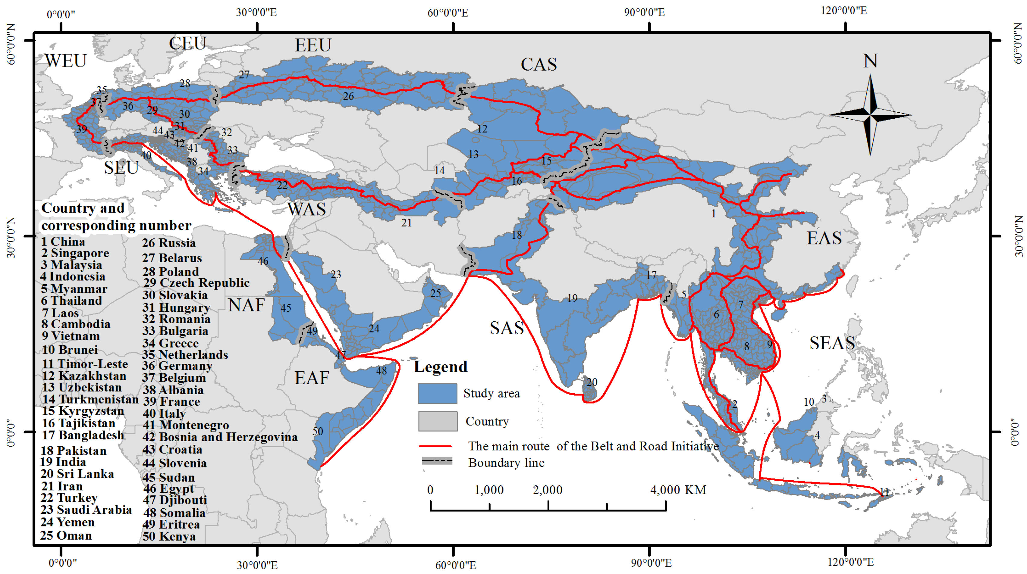
2.1. Study Area

The “Belt and Road” route refers to the main node cities and roads based on the “Belt and Road” initiative’s spatial pattern, the main route formed by the series of ports reflecting the trend of the “Belt and Road”. The main water-resource areas of the BRI refers to the main axis of the “Belt and Road” main route, and the borders of the national administrative regions or watershed boundaries along the line as the limits, with the water resource zones or administrative zones within the limits as the main water resource zone. The main water resources area composed of units reflecting the main route of the “Belt and Road”. This study took the main water-resource areas of the BRI as the research object (Figure 1). The total area of the study site extends between 00°04′ E−137°03′ E and 10°59′ S−58°57′ N. The study scope was based on the main BRI line drawn by Qiting Zuo [38]. Fifty countries in Asia, Europe, and Africa were included. These were further divided into 11 regions: East Asia (EAS), West Asia (WAS), South Asia (SAS), Central Asia (CAS), Southeast Asia (SEAS), Eastern Europe (EEU), Central Europe (CEU), Western Europe (WEU), Southern Europe (SEU), East Africa (EAF), and North Africa (NAF). Among them, the Asian region was divided into five parts involving 25 countries, the European region was divided into four parts involving 19 countries, and the African region was divided into two parts involving 6 countries.

2.2. Data

Land-use data for the main BRI water-resource areas were obtained for the years 2003, 2008, and 2013 from GLCNMO remote-sensing images (resolution: 500 m, https://globalmaps.github.io/glcnmo.html), issued by the Japan Geospatial Information Agency, Chiba University, and other cooperative organizations [39,40,41], and the data were widely used [42,43,44]. An accuracy of 500 m meets the needs of large-scale research and can ensure the reliability and authenticity of the remote sensing data.

2.3. Methods

2.3.1. Basis and Method for Classifying Land-Use Types

The research area covers a wide range of areas. The criteria for determining land-use types are not uniform throughout the world, and the definitions of classification types also differ among different classification systems [45]. Since there is a lack of comparability between them, it is necessary to find a unified classification standard, establish links between countries, and make it multisource. This study, therefore, aimed to establish an effective link between remote sensing data and land-use information from different global and regional projects, synthesize the relevant literature, and adopt the Food and Agriculture Organization of the United Nations/United Nations Environment Programmed Land Cover Classification System (FAO/UNEP LCCS) classification system. Based on the characteristics of different types of land cover, ArcGIS was used to reclassify it into nine large-scale land-use types: Forest, shrubland, grassland, cropland, wetland, bare land, urban, ice/snow, and water body (Table 1).

2.3.2. Calculation of Land-Use Dynamics

A dynamic degree model of land-use is normally used to express changes in land-resource quantity. Dynamic degree can quantitatively describe land-use change rates and truly reflect the intensity of land-use changes in a given region. A land-use dynamic degree model can be divided into single land-use dynamic degree and comprehensive land-use dynamic degree. This study used single land-use type dynamic degree R as an index for analysis [46]. Single land-use dynamic degree expresses the rate of quantitative change of a certain land-use type in a certain time range. Emphasis is placed on the change in individual land-use types, as expressed by the following:
R iT = U i b U i a U a × 1 T × 100 %
where RiT denotes the degree of land-use dynamic for a specific land-use type, Uia and Uib are areas that are annually under specific land-use types (km2), and T denotes time in years.

2.3.3. Land-Use Transfer Matrix

A land-use transfer matrix can be used to describe the structure and characteristics of land-use change in a study area and the direction of change among different land-use types. Its mathematical description is as follows:
S = ( S 11 S 1 n S n 1 S n n )
where S denotes areas, and n denotes the number of land-use types.

2.3.4. Comprehensive Index of Land-Use Degree

A comprehensive index of land-use degree quantitatively depicts the comprehensive effect of human activity on land-use change by assigning values to different land-use types, as expressed by the following equation [47]:
I = i = 1 n A i × C i
where I is the comprehensive index of land-use in the research area, Ai is the gradation value of the ith ranking land-use type, Ci is the area percentage of the ith ranking land-use intensity, and n is the land-use grade number.
The quantification of the degree of land-use is based on the limit of the degree of land-use, the upper limit of land-use, that is, the utilization of land resources reaches the peak, and human beings are generally unable to make further use and development of land resources, while the lower limit of land-use is the starting point for the development and utilization of land resources. Land-use classification system classifies land-use types according to remote sensing data, FAO/UNEPLCCS classification, main land-use patterns, and other factors. According to the natural balance maintenance state of land natural complex under the influence of social factors, it is divided into four kinds, which are Unused land grade; Forest, Grassland, and Water Land Grade; Agricultural Land Level; and Urban Settlement Land Level. Category values are given to four kinds of land-use grade, which results in four kinds of land-use degree classification indexes [48]. According to the land-use degree of the nine land-use types after classification, the corresponding grading index is obtained, as shown in Table 2.

2.3.5. Evaluation Method for Ecosystem Services

This study adopted the method of value evaluation based on monetary quantity. The result of the value evaluation method is monetary value. It can not only compare different ecosystems with the same ecosystem service, but also integrates the individual services of an ecosystem. Costanza et al. used it to analyze students in a region. ESV is calculated using the following equation:
ESV = A k × V C k
where ESV denotes ecosystem service value, Ak is the area (ha) for land-use type k, and VCk (seJ/ha) is the value coefficient for land-use type k. The value coefficients of the global ecosystem services of different land-use types were determined based on Costanza et al. [31].
In the last stage, we quantified the ESV of nine land-use types determined during the study period; because the ESV of different land-use types in different regions of the world are different, in order to quantify and unify, we used the method proposed by Costanza et al. [31] and Li et al. [33] to assess the ESV. Among them, the equivalent biological community corresponding to wetland, ice, forest, grassland, cropland, and urban is consistent, which corresponds to rock and lakes/rivers according to the definition and description of bare land and water body; the classification of land-use type in the ESV established by Costanza does not include shrubland, but shrubland belongs to woody plants, which is similar to forest, so the equivalent biological community of shrubland is defined as forest.
The biomes used as proxies for the land-use categories were not perfect matches. Specifically, the land-use settlement differed from Costanza et al. [31] urban biomes. For example, shrubland is not identical with forest as it lacks the desired level of canopy cover. We also used the values of rock ecosystem service as surrogate for the estimation of bare land.
Ecosystem functions are the characteristics of ecosystem services [49]. Therefore, these functions (see [39]) are used to determine which services are acquired/lost as the type of land cover changes over a specific period of time in the study landscape. According to Costanza, 17 ecosystem functions are divided into 4 ecosystem services and major related products can be found on the website of Bateman et al. [50]. The ecosystem functions are quantified to provide the number of ecosystem functions acquired/lost, and then used to further quantify the total ecosystem services acquired/lost.

3. Results

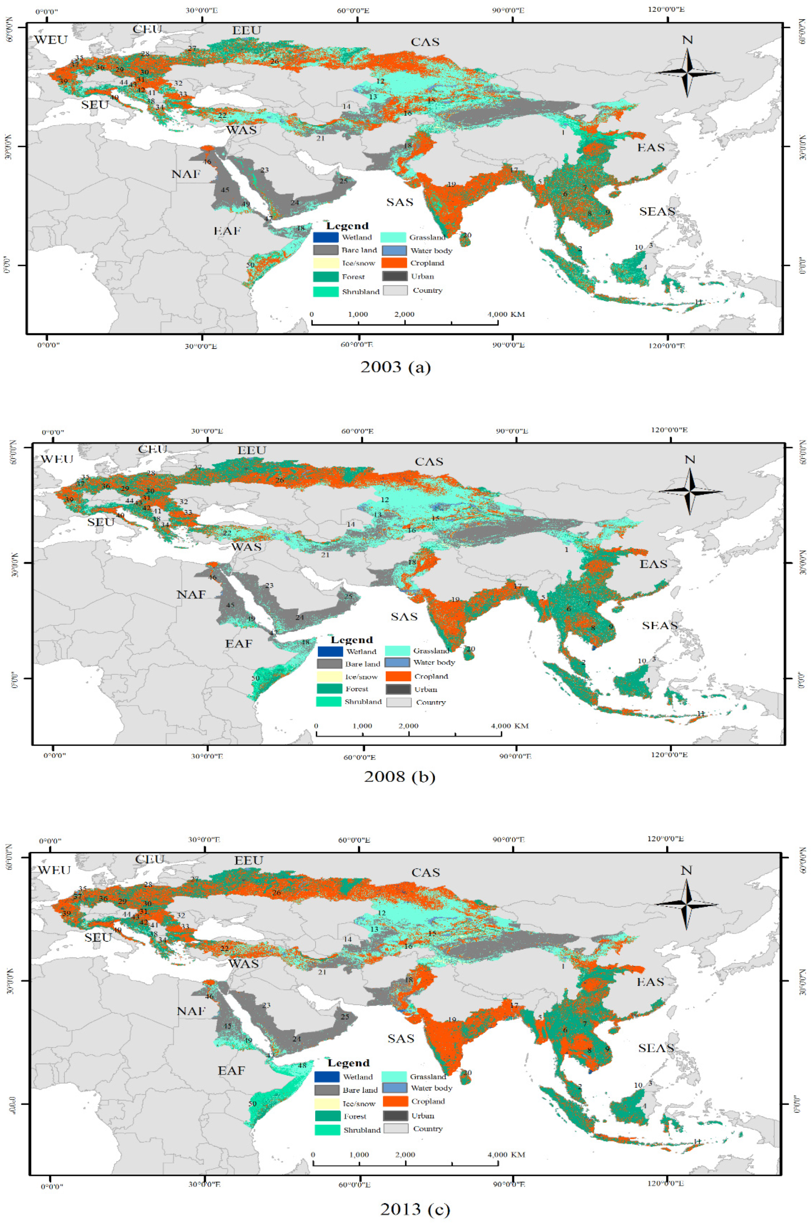
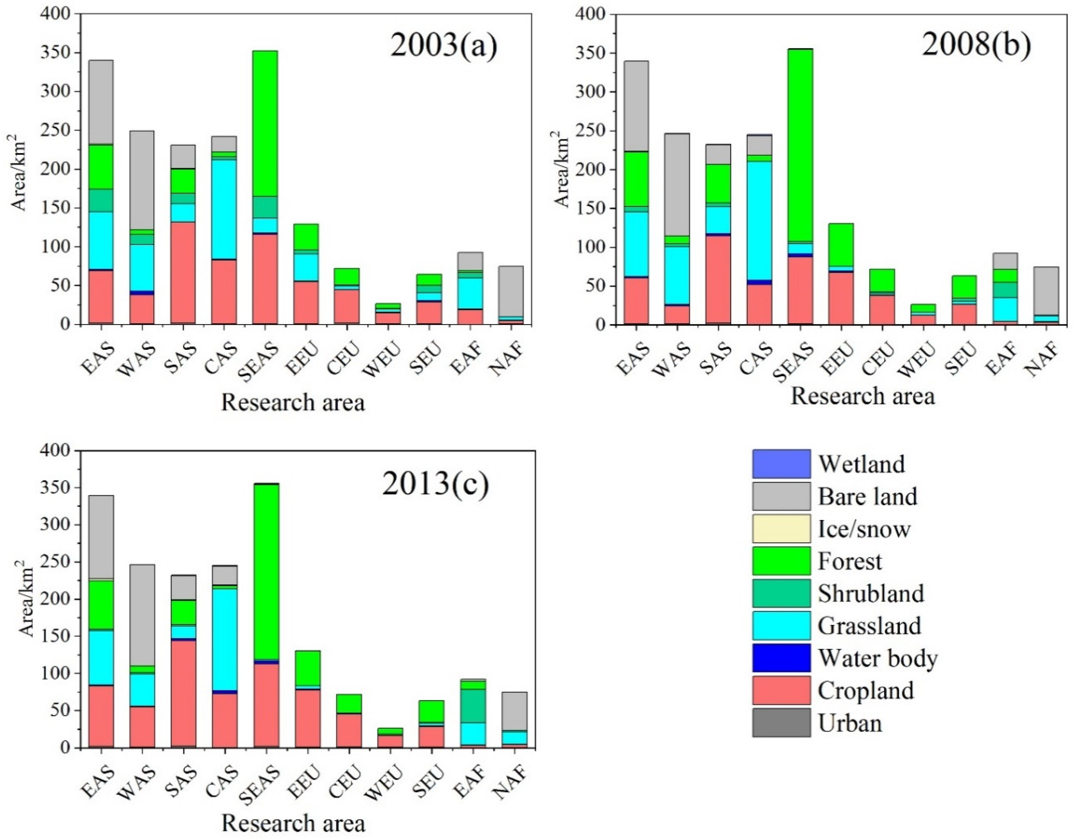
3.1. Land-Use Distribution Pattern of the Belt and Road Areas

Using the FAO/UNEP LCCS classification system, according to nine large-scale land-use types, data for 2003, 2008, and 2013 were analyzed by ArcGIS; then, land-use maps of BRI areas were obtained for the specified years (see Figure 2). It was found that during 2003–2013, cropland was the main land-use type, accounting for 27.28–35.36% of the total area. South Asia accounts for the largest proportion of cropland, and is located in the tropics, with sufficient heat, with the best land conditions in Asia, which leads the cropland areas. South Asia has one of the largest cropland areas of the world, both in terms of the net cropland area as well as the gross cropland area [51,52]. North Africa accounts for the least proportion of cropland, and most of its land-use types are bare land. Specifically, North Africa is dominated by tropical desert climate, with annual precipitation of about 200 mm, resulting in more than 70% bare land in North Africa [53].
This was followed by grassland, forest, and bare land, accounting for 18.93–23.32%, 17.76–25.98%, and 18.24–19.15% of the total area, respectively. The grassland area is mainly concentrated in EAS, WAS, and CAS, accounting for about 60% of the total grassland area. Forest is the main land-use type of SEAS. The abundant rainfall and frequent high temperature in SEAS have formed humid and hot climate characteristics, which provide extremely favorable conditions for the growth of tropical forests, making the region the most prosperous tropical forest in Asia and one of the most abundant tropical forest resources in the world [54]. Meanwhile, wetland, urban, ice/snow, and water body were all less, accounting for less than 1%.
The distributions of land-use in different regions of the study area were quite different (Figure 3). In 2003, the most prevalent land-use type was bare land in EAS, WAS, and NAF, accounting for 32%, 52%, and 87%, respectively. Grassland dominated in CAS and EAF. SEAS were mainly forest. EEU, CEU, WEU, and SEU had cropland as the main land-use type. In 2013, The main types of land-use in SEU have changed from cropland to forest. At this stage, human activities and climate change may affect the conversion of shrubland and grassland to forest, resulting in the forest area exceeding the cropland area. In EAF, the main land-use types have changed from grassland to shrubland. The main reason is that the change of cropland and bare land area has become shrubland. The decrease of bare land area is related to population expansion, but the change of cropland area to shrubland is not the same as the result of population growth, land-use policy change, and agricultural expansion [55]. The land-use types in the rest areas have not changed and remain stable.

3.2. Spatiotemporal Evolution of Land-Use in the Belt and Road Areas

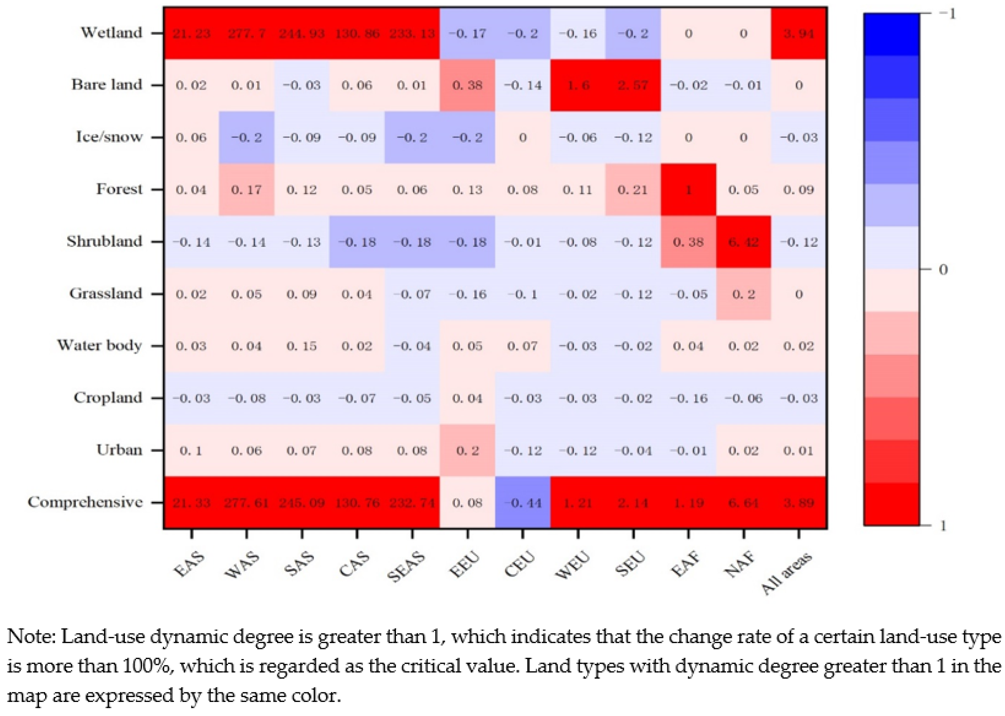
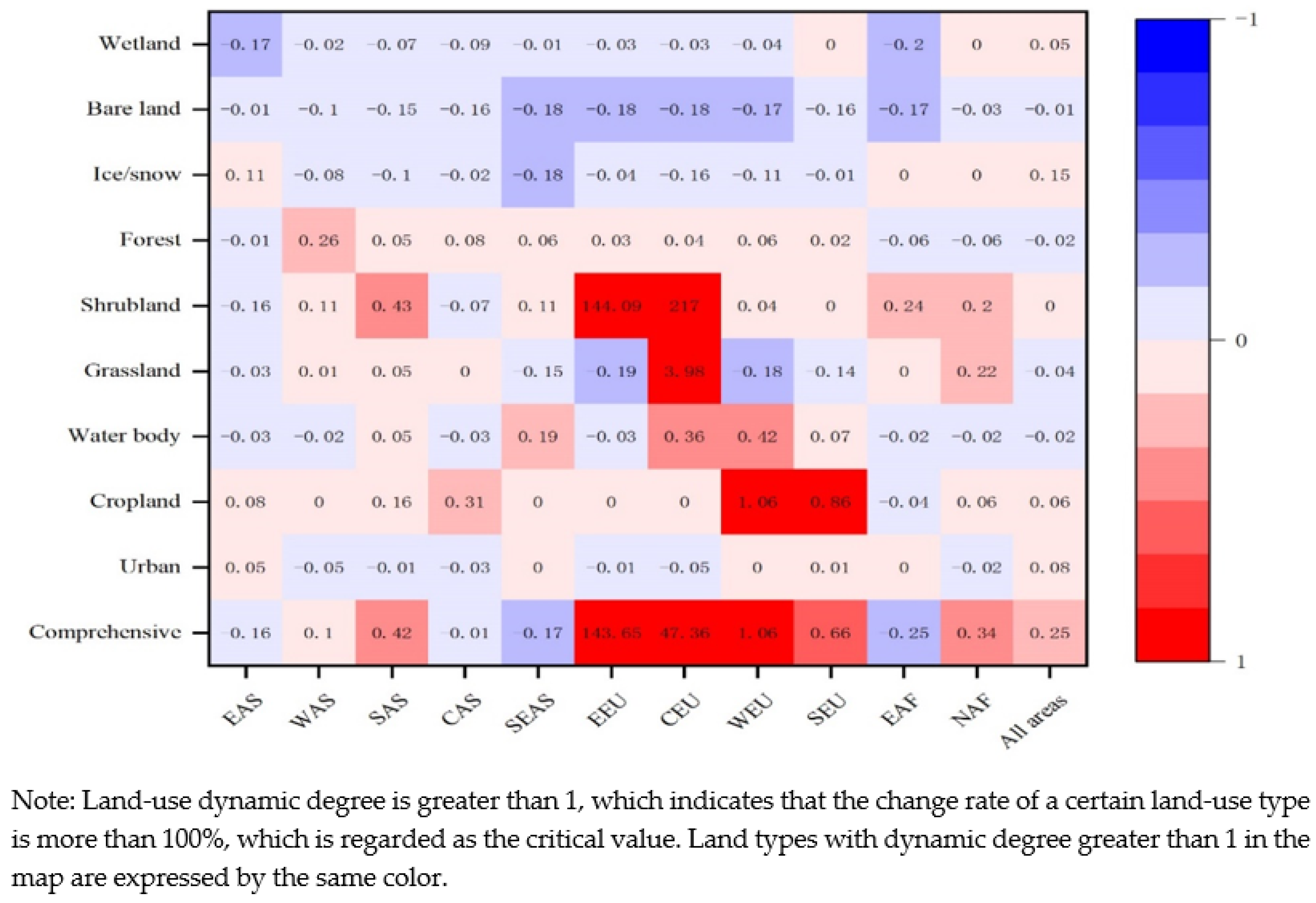
3.2.1. Dynamic Changes in Land-Use in the Belt and Road Areas

Dynamic degree can be used to judge the stability of land type in a given study period. Based on the single land-use dynamic degree formula, the land-use dynamic degrees (annual averages) of BRI areas and 11 districts during the periods 2003–2008 and 2008–2013 were calculated and illustrated in thermal maps (Figure 4).
There were significant differences in land-use changes in the study area. The maximum change in land-use dynamic degree was in wetland, up to 394%. Wetlands are among the most valuable ecosystems in the world due to their delivery of ESV, but they are particularly vulnerable to drivers of land-use change, especially within the scope of taking the main water resources area as the research area [56]. This indicates that wetland was the most active land-use type during 2003–2008. The smallest (at 0) were grassland and bare land, indicating that they were the most stable land-use types during 2003–2008. There were also significant differences in land-use changes among different zones. The largest change in comprehensive land-use dynamic degree was in WAS, reaching as high as 27,761%. The main reason for the change is that the areas of wetland in WAS were very small in 2003, and the increased area of wetland from 2003 to 2008 was much larger than the original, which made the wetland dynamic degree in WAS the largest. The next-largest changes were in SAS, SEAS, and CAS, while the smallest change was in EEU (only 8%).
In EEU, bare land showed the biggest change, reaching 38%, while cropland was the smallest at 4%. The dynamic degree of all land-use types was not more than 40%, which was relatively stable. In CEU, wetland showed the biggest change, reaching −20%, while ice/snow was the smallest at 0. The dynamic degree for all land-use types was relatively stable, with changes of no more than 20%. The biggest change in land-use dynamic degree in WEU was bare land (up to 160%), while the smallest was grassland at −2%; otherwise, the changes in land-use dynamic degree for other land-use types were not more than 16%, which was relatively stable. The biggest change in land-use dynamic degree in SEU was for bare land, up to 257%, while wetland was −2%. The largest land-use dynamic change in EAF was for forest, up to 100%, while wetland and ice/snow were the smallest (0); the dynamic degree for other land-use types was no more than 38%, which is relatively stable. In NAF, the largest dynamic degree of land-use change was for shrubland, up to 642%, while wetland and ice/snow were the smallest (0); other dynamic degree changes in land-use types were no more than 20% (i.e., relatively stable).
It can be seen that in Europe, the dynamic degree of bare land is greater than other land types, while in Asia, the dynamic degree of wetland is greater, because bare land and wetland area are relatively small in Europe and Asia.
The annual change rates in land-use type during 2008–2013 in BRI areas were calculated using the single land-use dynamic degree formula (Figure 5). The results showed no significant differences in land-use changes in the study area. The change in land-use dynamic degree was the largest, but only at 15%, indicating that the changes in the nine land-use types were relatively stable during 2008–2013. However, there were significant differences in land-use changes among different zones, among which the most significant was the comprehensive land-use dynamic degree in EEU, which was up to 14,365%; the smallest change was in CAS at only 1%. In the seven subregions of EAS, CAS, WAS, SEAS, SAS, EAF, and NAF, the largest changes in land-use dynamics were wetland, ice/snow, cropland, shrubland (grassland), wetland, shrubland, and shrubland, with sizes of −17%, 31%, 26%, 18%, 43%, 24%, and 20%, respectively. The degree of change was no more than 43%, and the overall change was relatively stable. The smallest change in land-use dynamics among the seven zones was forest (bare land), bare land, ice/snow, ice/snow, water body, shrubland (urban and ice/snow), wetland, and ice/snow.
By analyzing the overall and state land-use dynamics of the study area in 2003–2008 and 2008–2013, it can be found that the degree of land-use change (0.25) in 2008–2013 is more stable than that in 2003–2008 (3.89). In addition to EEU and CEU regions, the degree of land-use change in other regions is also stable. The change of wetland area between 2008–2013 in EEU and CEU is the main reason for the increase of regional dynamic degree.

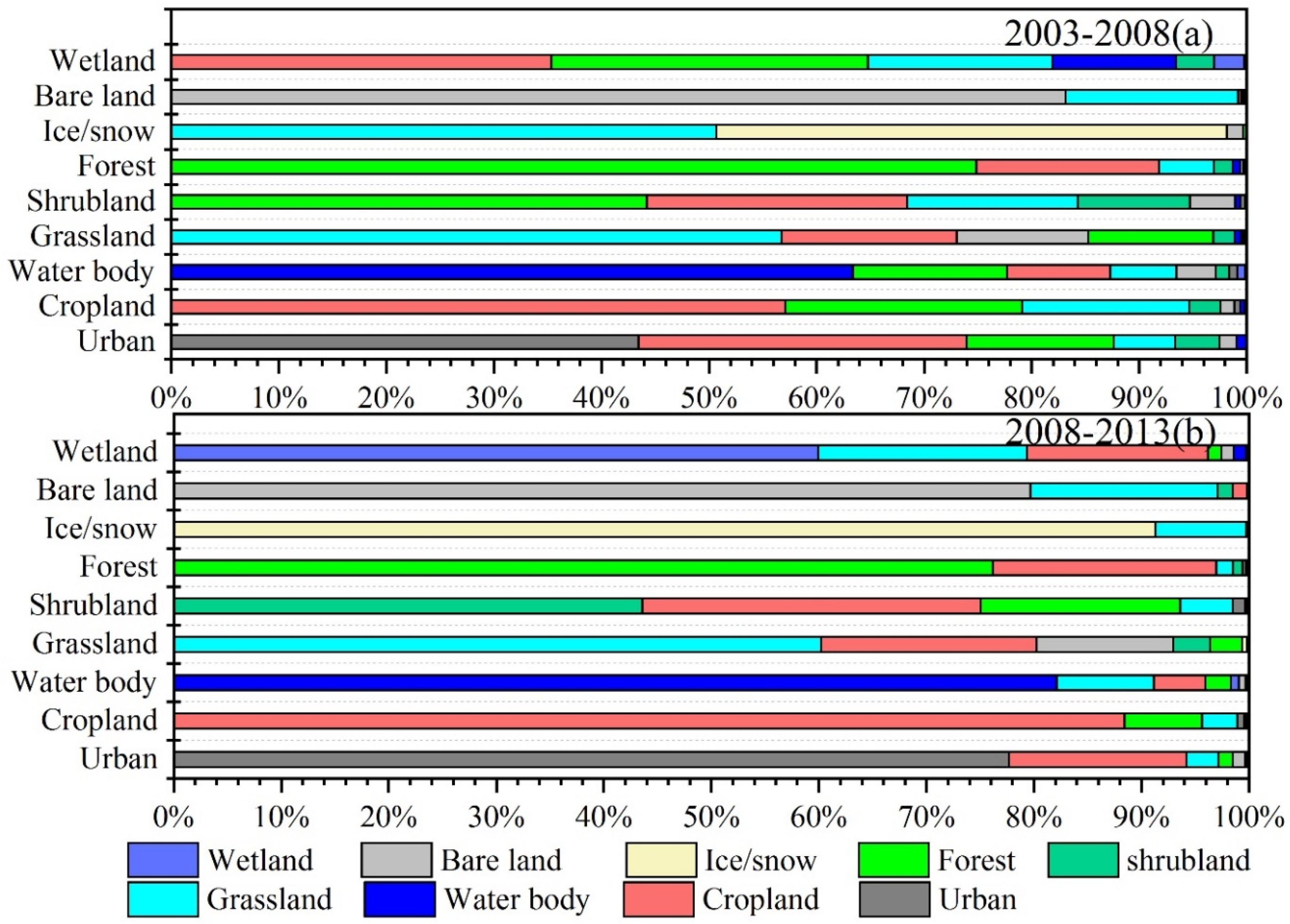
3.2.2. Land-Use Transfer Characteristics of the Belt and Road Areas

Formula (2) calculates the transfer matrices and land-use transfer matrices from 2003 to 2008 and 2008 to 2013 (Table 3 and Table 4). Table 3 shows the following main characteristics of land-use conversion in the study area during 2003–2008: (1) 1286 km2 of wetland was converted into other land types, and 28,142 km2 was converted into wetland; (2) a total of 591,098 km2 of bare land was converted into other land types, and 675,251 km2 was converted into bare land; (3) a total of 15,968 km2 of ice/snow was converted into other types and 11,793 km2 of other types into ice/snow; (4) 837,674 km2 of forest was transformed into other land types and 2,381,774 km2 of other land types into forest; (5) 955,386 km2 of shrubland was transformed into other land types and 336,206 km2 of other land types into shrubland; (6) 1,890,290 km2 of grassland was transformed into other land types and 1,897,577 km2 of other land types into grassland; (7) 68,013 km2 of water body was converted into other types and 87,761 km2 of other types into water body; (8) 2,651,823 km2 of cropland was transformed into other land types, while 1,590,277 km2 was converted into cropland; (9) 51,924 km2 of urban was converted into other land types and 54,676 km2 into urban types.
Table 4 shows that the main characteristics of land-use conversion in the study area during 2008–2013 were as follows: (1) 11,302 km2 of wetland was converted into other land types, and 18,819 km2 of other land types were converted into wetland; (2) 730,189 km2 of bare land was converted into other land types, and 561,646 km2 of other land types were converted into bare land; (3) in addition, 2293 km2 of ice/snow was converted into other types 22,195 km2 of other types into ice/snow; (4) 1,163,548 km2 of forest was transformed into other land types and 589,093 km2 of other land types into forest; (5) 252,692 km2 of shrubland was transformed into other land types and 256,234 km2 of other land types into shrubland; (6) 1,740,628 km2 of grassland was transformed into other land types and 918,839 km2 of other land types into grassland; (7) 37,448 km2 of water body was converted into other types and 16,129 km2 of other types into water body; (8) 591,863 km2 of cropland was transformed into other land types, and 2,110,373 km2 was converted into cropland; (9) meanwhile, 21,146 km2 of urban was converted into other land types, and 57,782 km2 of other land types were converted into other land types.
The analysis of land-use transfer rate (Figure 6) for 2003–2008 and 2008–2013 indicates that the main land-use change in the study area was the mutual transformation between forest, shrubland, cropland, grassland, and bare land. Meanwhile, the transformation between wetland, urban, ice/snow, and water body was relatively stable. From 2003 to 2008, the conversion of cropland to other land types was the largest, at 2,651,823 km2, of which 51.31%, 36.30%, 6.72%, and 2.94% were mainly converted into forest, grassland, shrubland, and bare land, respectively. The conversion of other land types to forest was the largest, at 2,381,774 km2, mainly from cropland, grassland, and shrubland, at 57.1%, 3%, 21.32%, and 19.81%, respectively. From 2008 to 2013, the conversion of grassland to other land types was the largest, at 1,740,628 km2, of which 50.32%, 31.90%, 8.69%, and 7.45% were mainly converted into cropland, bare land, shrubland, and forest, respectively. The conversion of other land types into cropland was the largest, at 2,110,373 km2, mainly from forest, grassland, shrubland, and bare land, with proportions of 50.32%, 31.90%, 8.69%, and 7.45%, respectively.

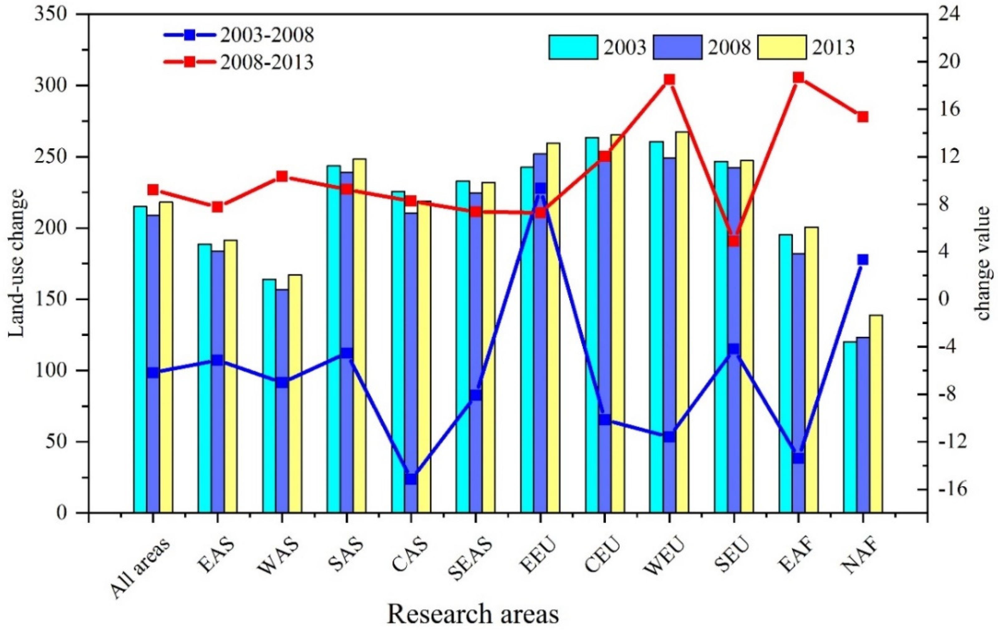
3.2.3. General Change Characteristics of Land-Use Degree in Study Area

Based on formula (3), the comprehensive index and change value of land-use degree of the study area and 11 districts were calculated for 2003, 2008, and 2013 (Figure 7). The influence degree of human activity on land-use in the two time periods was studied accordingly. The findings are described below.
During the period 2003–2018, the land-use degree of the study area showed a general downward trend; only EEU and NAF showed an upward trend. Thus, during this period, the proportion of land-use types that have a greater effect on human activity, such as artificial land surfaces and cropland, decreased, meaning humans have not made as much effort to transform nature. During the period 2008–2013, the land-use degree of the study area and all districts increased. This shows that during this period, land-use areas with low-intensity human activity (e.g., wetland, bare land, ice/snow) decreased, and human activity aimed at transforming nature intensified.
The change in land-use degree in EAS, WAS, SAS, CEU, WEU, SEU, EAF, and NAF during 2008–2013 was greater than during 2003–2008. This indicates that the land-use degree in these regions was affected by human activity, showing an upward trend. The changes in value in CAS, SEAS, and EEU during 2003–2008 were greater than during 2008–2013, indicating a decline in the degree of land-use affected by human activity.
During the study period, except for the decline of land-use composite index in central and Western Asia, the land-use composite index in other regions has been improved. It shows that most areas are increasingly affected by human activities, mainly manifested in the increase of cultivated land area conducive to human development, and the increase of forest area under the requirements of environmental protection. On the contrary, the area of wetland and grassland continues to decline.

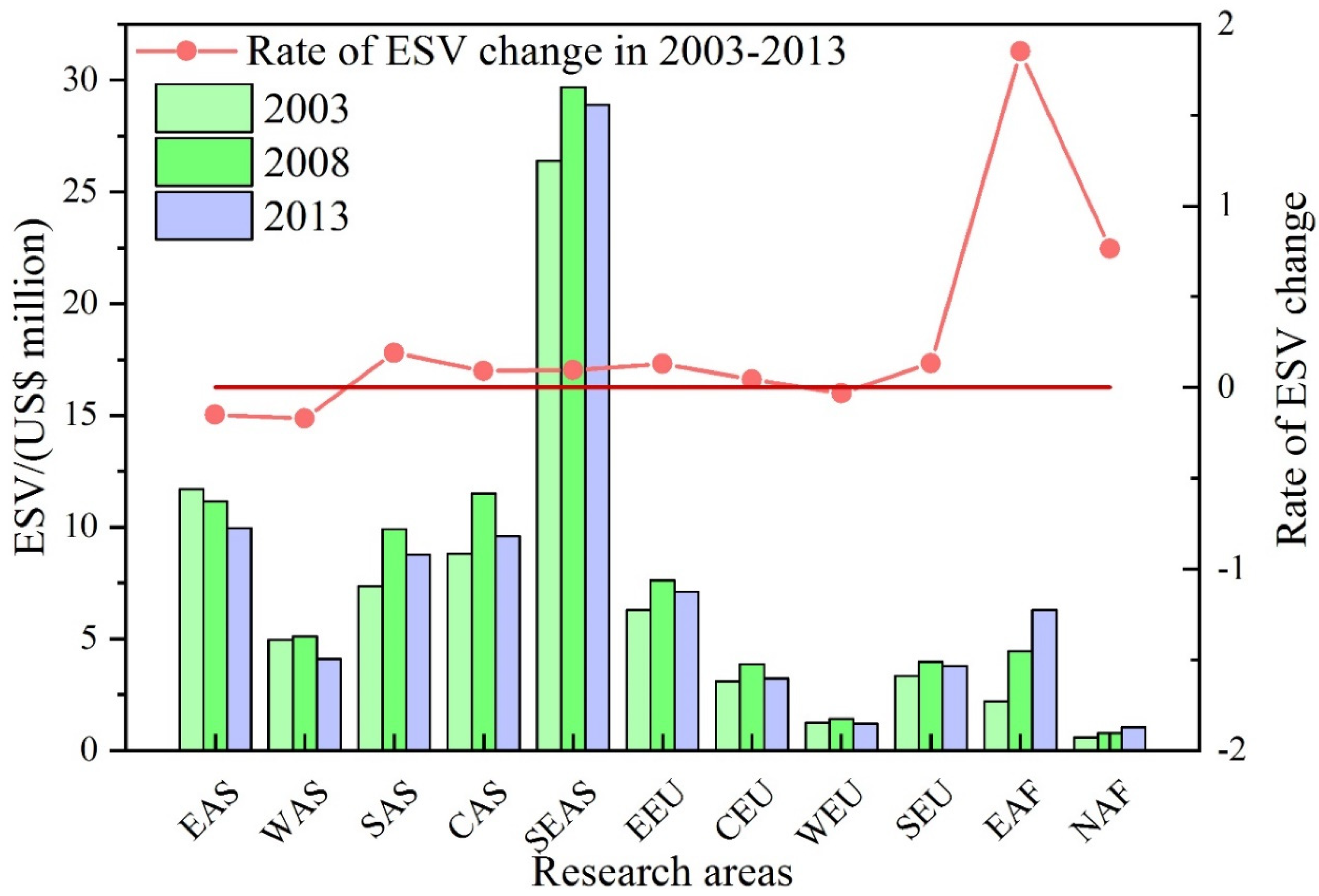
3.3. Changes in Ecosystem Services during the Period 2003–2013

Ecosystem service function is a general term for all kinds of environments needed by the ecosystem to maintain normal human development and survival. It is closely related to land-use change [57,58]. Formula 4 was used to calculate the overall ESV and the ESV of different land-use types in the study area in 2003, 2008, and 2013. The contributions of different land-use types to the total ESV differ. In general, forest ESV was the highest, accounting for the total price, with values ranging from 43% to 54%. The net ESV of the study area was increased by 9.52% over the one decade of the study period, from US $ 74.98 million in 2003 to US $ 82.12 million in 2013 (Table 5). In general, the main reason for this increase was afforestation and the increase in wetland (forest/wetland). However, at the same time, the reduction of shrubland and Grassland hindered the increase of ESV. In general, other land-use contribute little to ESV. In order to maximize ESV of landscape, it is very important to balance production and protection.
The estimated annual values of ecosystem functions and their changes are presented in Table 6. Four functions decreased their values during the study period, although it is inferior: Gas regulation (minus US $ 0.01 million), biological control (minus US $ 0.14 million), food production (minus US $ 0.07 million) and genetic resource (minus US $ 0.06 million) contributing most to the overall increase (minus US $ 0.01 million). All the other functions increased their values, with disturbance regulation (plus US $ 1.57 million), water supply (plus US $1.37 million), nutrient cycling (plus US $1.28 million), and waste treatment (plus US $1.05 million) contributing most to the overall decrease (plus US $7.16 million).
When the overall ecosystem functions in Table 6 are grouped under provisioning, supporting, regulating, and cultural services and the changes analyzed, all ecosystem services increased, but the most highly increased ecosystem service was regulating services. It can be understood from this finding that the dynamics of land-use over spatial and temporal scales can have a significant impact on the overall ESV at the landscape scale in general and on the forest, wetland, shrubland, and grassland cover types in particular.
The ESV of each area in 2003, 2008, and 2013 and the rate of ESV change are shown in Figure 8. The increase rate of ESV in EAF and NAF areas was larger (EAS: 185%, NAF: 76%), the change rate of ESV in other areas was not large, all maintained between −20% to 20%. It shows that during the study period, the land-use change in EAF and NAF areas tends to develop in the direction of better ecological environment. Among them, the ESV in the EAF, SEAS, and SAS regions increased greatly (EAF: 4.08, SEAS: 2.51, SAS: 1.41), while the ESV in the WAS and EAS regions decreased the most (EAS: −1.71, WAS: −0.85). Among them, the increase of the forest and shrubland in the EAF led to increase in ESV; the increase in the area of forest and wetland in the SEAS area led to an increase in ESV; the increase in the wetland in the SAS caused an increase in ESV. The decrease of ESV in the WAS and EAS area was mainly due to the decrease in shrubland. Through the ESV changes and land-use changes in each state, it can be found that the ESV changes in each state are greatly affected by the changes in forest, shrubland, and wetland. The forest and shrubland mainly changes in the area, although the wetland area changes a little, were the wetland higher ecological service value and greater impact on overall ecological value service. During the whole research period, food production and biological control did not increase with the increase of cultivated land, but at the same time, the decrease of grassland also restricted the increase of food production and biological control.

4. Discussions

4.1. Land-Use Change Analysis

During the period 2003–2013, the changes in land-use types in the study area were influenced by many factors. Though each factor has certain effects on land-use, these effects do not occur independently but are constrained by many other factors, including population change, urbanization level, and economic growth [59]. Especially in developing countries, population growth and economic expansion have been key factors influencing land-use changes. Land-use pattern and land-use change are the key to the sustainable development of developing countries, and the research area covers 50 countries, most of which are developing countries. Therefore, reasonable land-use change has a positive meaning for developing countries to achieve rapid economic and social development. However, urbanization, rural transformation, and the development of modern agriculture all over the world lead to population growth and economic expansion, and constantly affect land-use change [12,60].
A considerable increases of forest land was observed across the study period. This is in line with the increasing trend of forest resources worldwide. This has been evidenced by many studies [61,62]. The increase in forest area is due to the fact that more and more countries began to conduct forest inventory between 2003 and 2013 [63], including many country in the Belt and Road, which is also related to the concern of green belt development in the “one belt and one road” area [64]. In the two stages of 2003–2008 and 2008–2013, the forest area shows a trend of increasing first and then decreasing. The change trend between cultivated land area and forest area is opposite, which shows that under the influence of human activities, cultivated land area, and forest area have a mutual conversion relationship.
Among them, the expansion of urban area in 2003–2013 is related to urbanization and population growth. With the acceleration of global urbanization and population expansion, urban industrial development and housing demand as well as crop planting have a significant impact on the change of land-use [65]. Taking China as an example, as the largest developing country in the world, China is currently facing many challenges in land-use. China’s rapid urbanization, rural transformation, and the development of modern agriculture have many problems, including the transformation of productive cropland into real estate development, over intensification of agricultural land, land degradation, abandonment of cropland, the emergence of “hollow villages”, and land fragmentation, which cause soil land-use to change [65,66,67].
Increased population has intensified the effect of human activity, especially with regard to land-use types directly related to human activity, such as forest and cropland [68]. A larger population requires more cropland to grow food. This is especially true of most of the countries in the study area, which are mostly developing countries and require a certain guaranteed amount of cropland. Meanwhile, rapid economic development has led to a transfer of the labor force from rural to urban areas, along with accelerated urbanization, rapid enterprise development, and increased transportation demands. All of this has produced various changes in land types [69]. Accordingly, some countries have introduced relevant land policies. China, for example, has introduced various policies related to cropland and forestry to protect the environment [70], effectively changing the original development trends in land-use changes [10].

4.2. Ecosystem Services

In the study watershed, the total ESV showed an increases trend in the last 10 years. Particularly, from the correspond LULC dynamic over time, the ESV of forest, wetland, and cropland continuously increased with various proportions. The LULC dynamics were attributed to the improvement of these ESV. Changing shrubland and grassland to cultivated lands were common practice. Thus, the study suggested that the increases in ESVs were mainly connected to the change of shrubland and grassland into forest and cropland. The results showed that land-use change in the study area had a great impact on ecosystem service functions, especially the change of forest area, which has a great impact on the ability of ecosystem to continuously provide more ecosystem services [71]. The increase of forest area in the study area is mainly concentrated in Africa, and African governments are planning to promote reforestation or restoration programs in humid areas, so as to increase the forest area [72]. Most of the increases of ecological value services were related to the increase of wetland and forest. Although the value of ESV has increased in 2013 compared with that in 2003, it showed a downward trend from the development trend of 2008–2013, indicating that the main reason for the decline was also the decrease of forest and grassland area in the past five years, which is similar to the trend of global ESV in 2007 were US $145 trillion/year; however, it dropped to US $125 trillion/year in 2011 [73].
ESV of a forest can be priority in highlands because of limited agricultural fields and flat areas like the northern part of the Turkey. In another view, in the middle Asian regions around Republic of Uzbekistan, grassland is valuable because of animal husbandry. Although the value evaluation model of ecosystem services established by Costanza [31] and Li et al. [33] and others is evaluated uniformly within the scope of the BRI, there is a certain degree of uncertainty and criticism [74,75,76]. With the use of a unified standard for calculation, the inter-annual change trend is the same, which has reference significance for the research area in the next step to rationally plan land-use and enhance the corresponding ESV.

5. Conclusions

We have quantified the changes in land-use and ecosystem services in the main water-resource areas of the BRI. The research shows that in the two stages of 2003–2008 and 2008–2013, forest and cropland increased fastest. Large areas of wetland and shrubland were converted to urban, cropland, and bare land in the main water-resource areas of the BRI; to some extent, this led to the improvement of total ecosystem services in 2003–2013. Although a net increase in ESV of 8.69% (US $7.14 million) was found between 2003 and 2013, total ESV decreased from US $88.62 million to US $82.12 million (−7.3%) as a result of land-use change from 2008 to 2013. This indicates a concerning trend in sustainability of ecosystem services from the study area. This modest overall decline masks significant complexity and dynamics in the value of individual ecosystem services that occurred as some services displayed substantial decreases in value while others rose substantially. According to the results of the study, the managers should take corresponding measures to plan the land-use reasonably so as to make the ESV develop in a good and sustainable direction.
In this study, owing to the wide range and large area of the study area, the ESV generated by the same land-use type may be different among different sub regions, and the resulting ESV should therefore be used with caution. We suggest that future research should use RS images with much higher resolution and localized ESV coefficients. This paper focuses on the study of land-use change and spatial and temporal changes of ESV in the large scale (the BRI areas), as there is a lack of detailed analysis and discussion on the temporal and spatial variation of each sub region. At present, the results are based on the existing data analysis, and there is no further analysis and discussion on the driving factors that cause this change. The next step will be based on the existing data to analyze the driving factors of land-use change, establish a prediction model, and make an accurate prediction of the land-use change and the future ESV change in order to better implement the measures.
We can better understand the changes of land-use types of the BRI according to the analysis of the land-use change in 2003–2013. These changes are partly caused by environmental changes and partly by human activities. Based on these changes, managers can make better land-use management plans and make land-use changes towards the direction of sustainable development of mankind. At the same time, the land-use research in the BRI can provide a good case study, its assessment of land-use change and ESV can be applied to other developing regions of the world or the whole world, and its ESV changes can be evaluated. The research results are more meaningful for those areas with notable changes or unfavorable development direction.

Author Contributions

Conceptualization, Q.Z. and X.L.; methodology, Q.Z. and X.L.; resources, L.H.; data curation, X.L. and M.H.; writing—original draft preparation, Q.Z. and X.L.; writing—review and editing, Q.Z.; visualization, X.L. and L.H.; supervision, Q.Z.; project administration, M.H.; funding acquisition, Q.Z. All authors have read and agreed to the published version of the manuscript.

Funding

The research was supported by the Natural Sciences Foundation of China (No. 51779230 and U1803241).

Acknowledgments

We are very grateful to the Editor’s comments and suggestions. The provided comments have contributed substantially to improve the paper.

Conflicts of Interest

The authors declare no conflict of interest.

References

  1. National Development and Reform Commission, Ministry of Foreign Affairs, Ministry of Commerce. Vision and Action to Promote the co Construction of the Silk Road Economic Belt and the 21st Century Maritime Silk Road [N]. People’s Daily, 2015-03-29 (004). Available online: http://zhs.mofcom.gov.cn/article/xxfb/201503/20150300926644.shtml (accessed on 1 July 2020).
  2. Huang, Y. Understanding China’s Belt & Road Initiative: Motivation, framework and assessment. China Econ. Rev. 2016, 40, 314–321. [Google Scholar] [CrossRef]
  3. Yang, R.J.; Duan, N.; Shu, J.M.; Zhang, H.Y.; Jiaerheng, H.; Wang, H.; Zhang, L.B.; Qiao, Q.; Yin, W.L.; Zhang, Q.; et al. Ecological Civilization Construction Strategies in the Tianshan Mountain Northern Slope Economic Belt. Strateg. Study Chin. Acad. Eng. 2017, 19, 40. [Google Scholar] [CrossRef]
  4. Yu, H. Motivation behind China’s ‘One Belt, One Road’ Initiatives and Establishment of the Asian Infrastructure Investment Bank. J. Contemp. China 2016, 26, 353–368. [Google Scholar] [CrossRef]
  5. Chen, Y.; Li, Z.; Li, W.; Deng, H.; Shen, Y. Water and ecological security: Dealing with hydroclimatic challenges at the heart of China’s Silk Road. Environ. Earth Sci. 2016, 75, 881. [Google Scholar] [CrossRef]
  6. Hafeez, M.; Chunhui, Y.; Strohmaier, D.; Ahmed, M.; Jie, L. Does finance affect environmental degradation: Evidence from One Belt and One Road Initiative region? Environ. Sci. Pollut. Res. 2018, 25, 9579–9592. [Google Scholar] [CrossRef]
  7. Tianhong, L.; Wenkai, L.; Zhenghan, Q. Variations in ecosystem service value in response to land use changes in Shenzhen. Ecol. Econ. 2010, 69, 1427–1435. [Google Scholar] [CrossRef]
  8. Camacho-Valdéz, V.; Ruiz-Luna, A.; Ghermandi, A.; Nunes, P.A.L.D.; Ruiz-Luna, A. Valuation of ecosystem services provided by coastal wetlands in northwest Mexico. Ocean Coast. Manag. 2013, 78, 1–11. [Google Scholar] [CrossRef]
  9. Wang, W.; Guo, H.; Chuai, X.; Dai, C.; Lai, L.; Zhang, M. The impact of land use change on the temporospatial variations of ecosystems services value in China and an optimized land use solution. Environ. Sci. Policy 2014, 44, 62–72. [Google Scholar] [CrossRef]
  10. Grainger, A.; Konteh, W. Autonomy, ambiguity and symbolism in African politics: The development of forest policy in Sierra Leone. Land Use Policy 2007, 24, 42–61. [Google Scholar] [CrossRef]
  11. Veldkamp, A.; Fresco, L. Reconstructing land use drivers and their spatial scale dependence for Costa Rica (1973 and 1984). Agric. Syst. 1997, 55, 19–43. [Google Scholar] [CrossRef]
  12. Yao, S.; Luo, D.; Wang, J. Housing Development and Urbanisation in China. World Econ. 2013, 37, 481–500. [Google Scholar] [CrossRef] [Green Version]
  13. Poelmans, L.; Van Rompaey, A. Complexity and performance of urban expansion models. Comput. Environ. Urban Syst. 2010, 34, 17–27. [Google Scholar] [CrossRef]
  14. Lambin, E.F.; Turner, B.L.; Geist, H.J.; Agbola, S.B.; Angelsen, A.; Bruce, J.W.; Coomes, O.T.; Dirzo, R.; Fischer, G.; Folke, C.; et al. The causes of land-use and land-cover change: Moving beyond the myths. Glob. Environ. Chang. 2001, 11, 261–269. [Google Scholar] [CrossRef]
  15. Johnson, R.D.; Kasischke, E.S. Change vector analysis: A technique for the multispectral monitoring of land cover and condition. Int. J. Remote Sens. 1998, 19, 411–426. [Google Scholar] [CrossRef]
  16. Takada, T.; Miyamoto, A.; Hasegawa, S.F. Derivation of a yearly transition probability matrix for land-use dynamics and its applications. Landsc. Ecol. 2009, 25, 561–572. [Google Scholar] [CrossRef]
  17. Liu, J.Y.; Liu, M.L.; Zhuang, D.F.; Zhang, Z.X.; Deng, X.Z. Study on spatial pattern of land-use change in China during 1995-2000. Sci. China Ser. D Earth Sci. 2003, 46, 373–384. [Google Scholar]
  18. Liu, J.; Kuang, W.; Zhang, Z.; Xu, X.; Qin, Y.; Ning, J.; Zhou, W.; Zhang, S.; Li, R.; Yan, C.; et al. Spatiotemporal characteristics, patterns, and causes of land-use changes in China since the late 1980s. J. Geogr. Sci. 2014, 24, 195–210. [Google Scholar] [CrossRef]
  19. Saini, R.; Aswal, P.; Tanzeem, M.; Saini, S.S. Land Use Land Cover Change Detection using Remote Sensing and GIS in Srinagar, India. Int. J. Comput. Appl. 2019, 178, 42–50. [Google Scholar] [CrossRef]
  20. Wang, G.Q.; Wang, S.Y.; Chen, Z.X. Land-use/land-cover changes in the Yellow River basin. J. Tsinghua Univ. 2004, 44, 1218–1222. [Google Scholar]
  21. Mooney, H.A.; Duraiappah, A.; Larigauderie, A. Evolution of natural and social science interactions in global change research programs. Proc. Natl. Acad. Sci. USA 2013, 110, 3665. [Google Scholar] [CrossRef] [Green Version]
  22. Turner, B.; Skole, D.; Sanderson, S.; Fischer, G.; Fresco, L. Land-Use and Land-Cover Change: Science/research plan. Glob. Chang. Rep. 1995, 43, 669–679. [Google Scholar]
  23. Sterling, S.M.; Ducharne, A.; Polcher, J. The impact of global land-cover change on the terrestrial water cycle. Nat. Clim. Chang. 2012, 3, 385–390. [Google Scholar] [CrossRef]
  24. Nelson, E.; Mendoza, G.; Regetz, J.; Polasky, S.; Tallis, H.; Cameron, D.; Chan, K.M.A.; Daily, G.C.; Goldstein, J.; Kareiva, P.M.; et al. Modeling multiple ecosystem services, biodiversity conservation, commodity production, and tradeoffs at landscape scales. Front. Ecol. Environ. 2009, 7, 4–11. [Google Scholar] [CrossRef]
  25. Burkhard, B.; Kroll, F.; Nedkov, S.; Müller, F. Mapping ecosystem service supply, demand and budgets. Ecol. Indic. 2012, 21, 17–29. [Google Scholar] [CrossRef]
  26. Polasky, S.; Nelson, E.; Pennington, D.; Johnson, K.A. The Impact of Land-Use Change on Ecosystem Services, Biodiversity and Returns to Landowners: A Case Study in the State of Minnesota. Environ. Resour. Econ. 2010, 48, 219–242. [Google Scholar] [CrossRef]
  27. Wan, L.; Ye, X.; Lee, J.; Lu, X.; Zheng, L.; Wu, K. Effects of urbanization on ecosystem service values in a mineral resource-based city. Habitat Int. 2015, 46, 54–63. [Google Scholar] [CrossRef]
  28. Kubiszewski, I.; Costanza, R.; Anderson, S.J.; Sutton, P.C. The future value of ecosystem services: Global scenarios and national implications. Ecosyst. Serv. 2017, 26, 289–301. [Google Scholar] [CrossRef]
  29. Wolff, S.; Schulp, C.J.; Verburg, P.H. Mapping ecosystem services demand: A review of current research and future perspectives. Ecol. Indic. 2015, 55, 159–171. [Google Scholar] [CrossRef]
  30. Liu, W.; Zhan, J.; Zhao, F.; Yan, H.; Zhang, F.; Wei, X. Impacts of urbanization-induced land-use changes on ecosystem services: A case study of the Pearl River Delta Metropolitan Region, China. Ecol. Indic. 2019, 98, 228–238. [Google Scholar] [CrossRef]
  31. Costanza, R.; D’Arge, R.; De Groot, R.; Farber, S.; Grasso, M.; Hannon, B.; Limburg, K.; Naeem, S.; O’Neill, R.V.; Paruelo, J.; et al. The value of the world’s ecosystem services and natural capital. Nature 1997, 387, 253–260. [Google Scholar] [CrossRef]
  32. Kreuter, U.P.; Harris, H.G.; Matlock, M.D.; Lacey, R.E. Change in ecosystem service values in the San Antonio area, Texas. Ecol. Econ. 2001, 39, 333–346. [Google Scholar] [CrossRef]
  33. Li, R.-Q.; Dong, M.; Cui, J.-Y.; Zhang, L.-L.; Cui, Q.-G.; He, W.-M. Quantification of the Impact of Land-Use Changes on Ecosystem Services: A Case Study in Pingbian County, China. Environ. Monit. Assess. 2007, 128, 503–510. [Google Scholar] [CrossRef] [PubMed]
  34. Kubiszewski, I.; Costanza, R.; Dorji, L.; Thoennes, P.; Tshering, K. An initial estimate of the value of ecosystem services in Bhutan. Ecosyst. Serv. 2013, 3, e11–e21. [Google Scholar] [CrossRef]
  35. Bateman, I.J.; Harwood, A.R.; Mace, G.; Watson, R.T.; Abson, D.J.; Andrews, B.; Binner, A.; Crowe, A.; Day, B.H.; Dugdale, S.; et al. Bringing Ecosystem Services into Economic Decision-Making: Land Use in the United Kingdom. Science 2013, 341, 45–50. [Google Scholar] [CrossRef] [PubMed]
  36. Lawler, J.J.; Lewis, D.J.; Nelson, E.; Plantinga, A.J.; Polasky, S.; Withey, J.C.; Helmers, D.P.; Martinuzzi, S.; Pennington, D.; Radeloff, V.C. Projected land-use change impacts on ecosystem services in the United States. Proc. Natl. Acad. Sci. USA 2014, 111, 7492. [Google Scholar] [CrossRef] [Green Version]
  37. Ouyang, Z.; Zheng, H.; Xiao, Y.; Polasky, S.; Liu, J.; Xu, W.; Wang, Q.; Zhang, L.; Rao, E.; Jiang, L.; et al. Improvements in ecosystem services from investments in natural capital. Science 2016, 352, 1455–1459. [Google Scholar] [CrossRef]
  38. Zuo, Q.T.; Han, C.H.; Hao, L.G.; Wang, H.J.; Ma, J.X. The main route and water resource areas of the Belt and Road Initiative. Resour. Sci. 2018, 40, 134–143. [Google Scholar]
  39. Tateishi, R.; Uriyangqai, B.; Al-Bilbisi, H.; Ghar, M.A.; Tsend-Ayush, J.; Kobayashi, T.; Kasimu, A.; Hoan, N.T.; Shalaby, A.; Alsaaideh, B.; et al. Production of global land cover data—GLCNMO. Int. J. Digit. Earth 2011, 4, 22–49. [Google Scholar] [CrossRef]
  40. Tateishi, R.; Hoan, N.T.; Kobayashi, T.; Alsaaideh, B.; Tana, G.; Phong, D.X. Production of Global Land Cover Data—GLCNMO2008. J. Geogr. Geol. 2014, 6, 99. [Google Scholar] [CrossRef] [Green Version]
  41. Kobayashi, T.; Tateishi, R.; Alsaaideh, B.; Sharma, R.C.; Wakaizumi, T.; Miyamoto, D.; Bai, X.L.; Long, B.D.; Gegentana, G.; Maitiniyazi, A.; et al. Production of Global Land Cover Data—GLCNMO2013. J. Geogr. Geol. 2017, 9, 1–15. [Google Scholar] [CrossRef] [Green Version]
  42. Gong, P.; Wang, J.; Yu, L.; Zhao, Y.; Zhao, Y.; Liang, L.; Niu, Z.; Huang, X.; Fu, H.; Liu, S.; et al. Finer resolution observation and monitoring of global land cover: First mapping results with Landsat TM and ETM+ data. Int. J. Remote Sens. 2012, 34, 2607–2654. [Google Scholar] [CrossRef] [Green Version]
  43. Zhang, Z.; Wang, X.; Zhao, X.; Liu, B.; Yi, L.; Zuo, L.; Wen, Q.; Liu, F.; Xu, J.; Hu, S. A 2010 update of National Land Use/Cover Database of China at 1:100000 scale using medium spatial resolution satellite images. Remote Sens. Environ. 2014, 149, 142–154. [Google Scholar] [CrossRef]
  44. Zhao, Y.; Gong, P.; Yu, L.; Hu, L.; Li, X.; Li, C.; Zhang, H.; Zheng, Y.; Wang, J.; Zhao, Y.; et al. Towards a common validation sample set for global land-cover mapping. Int. J. Remote Sens. 2014, 35, 4795–4814. [Google Scholar] [CrossRef]
  45. Zhang, J.H.; Feng, Z.M.; Jiang, L.G. Progress on studies of land use/land cover classification systems. Resour. Sci. 2011, 33, 1195–1203. [Google Scholar]
  46. Gao, P.; Niu, X.; Wang, B.; Zheng, Y. Land use changes and its driving forces in hilly ecological restoration area based on gis and rs of northern china. Sci. Rep. 2015, 5, 11038. [Google Scholar] [CrossRef] [Green Version]
  47. Quan, B.; Chen, J.-F.; Qiu, H.-L.; Römkens, M.; Yang, X.; Jiang, S.-F.; Li, B.-C. Spatial-Temporal Pattern and Driving Forces of Land Use Changes in Xiamen. Pedosphere 2006, 16, 477–488. [Google Scholar] [CrossRef]
  48. Liu, J.Y. Macro Survey and Dynamic Research of China’s Resources and Environment Remote Sensing; Science and Technology of China Press: Beijing, China, 1996. [Google Scholar]
  49. Haines-Young, R.H.; Potschin, M.; Kienast, F. Indicators of ecosystem service potential at European scales: Mapping marginal changes and trade-offs. Ecol. Indic. 2012, 21, 39–53. [Google Scholar] [CrossRef]
  50. Bateman, I.J.; Mace, G.; Fezzi, C.; Atkinson, G.; Turner, K. Economic Analysis for Ecosystem Service Assessments. Environ. Resour. Econ. 2010, 48, 177–218. [Google Scholar] [CrossRef] [Green Version]
  51. Gumma, M.K.; Thenkabail, P.; Teluguntla, P.G.; Oliphant, A.; Xiong, J.; Giri, C.; Pyla, V.; Dixit, S.; Whitbread, A. Agricultural cropland extent and areas of South Asia derived using Landsat satellite 30-m time-series big-data using random forest machine learning algorithms on the Google Earth Engine cloud. GIScience Remote Sens. 2019, 57, 302–322. [Google Scholar] [CrossRef] [Green Version]
  52. Thenkabail, P.S.; Knox, J.W.; Ozdogan, M.; Gumma, M.K.; Congalton, R.G.; Wu, Z.T.; Milesi, C.; Finkral, A.; Marshall, M.; Mariotto, I.; et al. Assessing Future Risks to Agricultural Productivity, Water Resources and Food Security: How Can Remote Sensing Help? Photogramm. Eng. Remote Sens. 2012, 78, 773–782. [Google Scholar]
  53. Wei, Y.; Lu, M.; Wu, W.; Ru, Y. Multiple factors influence the consistency of cropland datasets in Africa. Int. J. Appl. Earth Obs. Geoinf. 2020, 89, 102087. [Google Scholar] [CrossRef]
  54. Miettinen, J.; Wong, C.M.; ChinLiew, S. 500M spatial resolution land cover map in insular Southeast Asia. In Proceedings of the 2009 IEEE International Geoscience and Remote Sensing Symposium, Cape Town, South Africa, 12–17 July 2009; pp. III-314–III-317. [Google Scholar]
  55. Andreas, B.B.; Hugh, D.E. The potential use of high-resolution Landsat satellite data for detecting land-cover change in the Greater Horn of Africa. Afr. Geogr. Rev. 2015, 33, 209–231. [Google Scholar]
  56. Ricaurte, L.F.; Olaya-Rodríguez, M.H.; Cepeda-Valencia, J.; Lara, D.; Arroyave-Suárez, J.; Finlayson, C.M.; Palomo, I. Future impacts of drivers of change on wetland ecosystem services in Colombia. Glob. Environ. Chang. 2017, 44, 158–169. [Google Scholar] [CrossRef]
  57. Martínez-Harms, M.J.; Balvanera, P. Methods for mapping ecosystem service supply: A review. Int. J. Biodivers. Sci. Ecosyst. Serv. Manag. 2012, 8, 17–25. [Google Scholar] [CrossRef]
  58. Deng, X.; Li, Z.; Gibson, J. A review on trade-off analysis of ecosystem services for sustainable land-use management. J. Geogr. Sci. 2016, 26, 953–968. [Google Scholar] [CrossRef] [Green Version]
  59. Xu, X.; Liu, J. Analysis on spatial-temporal characteristics and driving force of land-use change in Hainan island. In Proceedings of the 2003 IEEE International Geoscience and Remote Sensing Symposium, IGARSS 2003, Toulouse, France, 21–25 July 2003; Volume 2644, pp. 2641–2643. [Google Scholar]
  60. Seto, K. The Routledge Handbook of Urbanization and Global Environmental Change; Informa UK Limited: London, UK, 2015. [Google Scholar]
  61. Adams, M.A.; Pfautsch, S. Grand Challenges: Forests and Global Change. Front. For. Glob. Chang. 2018, 1, 1. [Google Scholar] [CrossRef] [Green Version]
  62. FAO. State of the World’s Forests 2016. Forests and agriculture: Land-use challenges and opportunities. Food Agric. Organ. U. N. Rome 2016, 105–107. [Google Scholar]
  63. MacDicken, K.G.; Sola, P.; Hall, J.E.; Sabogal, C.; Tadoum, M.; De Wasseige, C. Global progress toward sustainable forest management. For. Ecol. Manag. 2015, 352, 47–56. [Google Scholar] [CrossRef] [Green Version]
  64. Dong, Z.F.; Ge, C.Z.; Wang, J.N.; Yan, X.D.; Cheng, C.Y. The strategic implementation framework of “The Belt and Road” green development. China Environ. Manag. 2016, 8, 31–35. [Google Scholar]
  65. Xie, H. Towards Sustainable Land Use in China: A Collection of Empirical Studies. Sustainability 2017, 9, 2129. [Google Scholar] [CrossRef] [Green Version]
  66. Xie, H.; He, Y.; Xie, X. Exploring the factors influencing ecological land change for China’s Beijing–Tianjin–Hebei Region using big data. J. Clean. Prod. 2017, 142, 677–687. [Google Scholar] [CrossRef]
  67. Xie, H.; Lu, H. Impact of land fragmentation and non-agricultural labor supply on circulation of agricultural land management rights. Land Use Policy 2017, 68, 355–364. [Google Scholar] [CrossRef]
  68. Zhang, H.Y.; Yang, D.G.; Shi, J.J.; Cai, W.C. Analysis on Land Use Change and Driving Force in Urumqi. J. Arid Land Resour. Environ. Resour. Econ. 2007, 21, 96–100. [Google Scholar]
  69. Lambin, E.F.; Meyfroidt, P. Global land use change, economic globalization, and the looming land scarcity. Proc. Natl. Acad. Sci. USA 2011, 108, 3465. [Google Scholar] [CrossRef] [Green Version]
  70. Long, H. Land use policy in China: Introduction. Land Use Policy 2014, 40, 1–5. [Google Scholar] [CrossRef]
  71. Laurance, W.F. Reflections on the tropical deforestation crisis. Biol. Conserv. 1999, 91, 109–117. [Google Scholar] [CrossRef]
  72. Catinot, R. Tropical silviculture in dense African forest (Part 1). Bois Forets Trop. 2018, 336, 7–18. [Google Scholar] [CrossRef]
  73. Costanza, R.; De Groot, R.; Sutton, P.C.; Van Der Ploeg, S.; Anderson, S.J.; Kubiszewski, I.; Farber, S.; Turner, R.K. Changes in the global value of ecosystem services. Glob. Environ. Chang. 2014, 26, 152–158. [Google Scholar] [CrossRef]
  74. Knoke, T.; Steinbeis, O.-E.; Bösch, M.; Roman-Cuesta, R.M.; Burkhardt, T. Cost-effective compensation to avoid carbon emissions from forest loss: An approach to consider price–quantity effects and risk-aversion. Ecol. Econ. 2011, 70, 1139–1153. [Google Scholar] [CrossRef]
  75. Wang, X.; Dong, X.; Liu, H.; Wei, H.; Fan, W.; Lu, N.; Xu, Z.; Ren, J.; Xing, K. Linking land use change, ecosystem services and human well-being: A case study of the Manas River Basin of Xinjiang, China. Ecosyst. Serv. 2017, 27, 113–123. [Google Scholar] [CrossRef]
  76. Kindu, M.; Schneider, T.; Teketay, D.; Knoke, T. Changes of ecosystem service values in response to land use/land cover dynamics in Munessa–Shashemene landscape of the Ethiopian highlands. Sci. Total. Environ. 2016, 547, 137–147. [Google Scholar] [CrossRef] [PubMed]
Figure 1. The main water resources area of “The Belt and Road” (study area).
Sustainability 12 06583 g001
Figure 2. Land-use map of study area in 2003 (a), 2008 (b), and 2013 (c).
Sustainability 12 06583 g002
Figure 3. Distribution maps of land-use types of study area in 2003 (a), 2008 (b), and 2013 (c).
Sustainability 12 06583 g003
Figure 4. The dynamics of land-use from 2003 to 2008 in study area.
Sustainability 12 06583 g004
Figure 5. The dynamics of land-use from 2008 to 2013 in study area.
Sustainability 12 06583 g005
Figure 6. Transfer rate of land-use type from 2003 to 2013.
Sustainability 12 06583 g006
Figure 7. Comprehensive index and change value of land-use degree in study area.
Sustainability 12 06583 g007
Figure 8. The ESV of each area and the rate of ESV change.
Sustainability 12 06583 g008
Table 1. Land-use classification table.
FAO/UNEP LCCS Classification SystemLand-Use Types
WetlandWetland
Bare area, consolidated (gravel, rock); Bare area, unconsolidated (sand)Bare area
Ice/SnowIce/snow
Broadleaf Evergreen Forest, Broadleaf Deciduous Forest, Needleleaf Evergreen Forest, Needleleaf Deciduous Forest, Mixed Forest, Tree Open, MangroveForest
Shrub, Sparse vegetationShrubland
Herbaceous, Herbaceous with Sparse Tree/ShrubGrassland
Water bodyWater body
Cropland, Paddy field, Cropland/Other Vegetation MosaicCropland
UrbanUrban
Table 2. Costanza biome equivalents for the land-use categories identified in this study, corresponding ecosystem services value (ESV), and land-use classification index table.
Land-Use TypesClassification Types of Land-UseGraded IndexEquivalent BiomesEcosystem Services Coefficient (US $ ha−1 year−1)
WetlandUnused land grade1Wetland14785
Bare landUnused land grade1Rock0
Ice/snowUnused land grade1Ice0
ForestForest, Grass and Water Land Grade2Forest969
ShrublandForest, Grass and Water Land Grade2Forest969
GrasslandForest, Grass and Water Land Grade2Grass/rangelands232
Water bodyForest, Grass and Water Land Grade2Lakes/rivers8498
CroplandAgricultural Land Level3Cropland92
UrbanUrban Settlement Land Level4Urban0
Table 3. Land-use situation transition matrix in study area from 2003 to 2008 (104 km2).
TypeWetlandBare LandIce/SnowForestShrublandGrasslandWater BodyCroplandUrbanTotal
Wetland0.000.000.000.040.000.020.020.050.000.13
Bare land0.12291.840.040.190.6156.340.600.930.29350.96
Ice/snow0.000.051.440.010.001.540.000.000.003.04
Forest0.530.890.13249.545.8816.992.3356.530.48333.30
Shrubland0.164.490.0047.1811.1516.930.5425.80.43106.68
Grassland0.7953.480.9950.788.70247.942.6071.130.56436.97
Water body0.140.690.032.660.231.1411.781.790.1418.6
Cropland1.077.790.00136.0717.8296.272.61352.963.56618.15
Urban0.000.140.001.260.380.530.092.803.999.99
Total 2.81359.372.63487.7344.77437.7020.57511.999.451877
Table 4. Land-use situation transition matrix in study area from 2008 to 2013 (104 km2).
TypeWetlandBare landIce/SnowForestShrublandGrasslandWater BodyCroplandUrbanTotal
Wetland1.690.030.010.040.000.550.030.470.002.82
Bare land0.18286.20.100.135.1062.480.184.800.04359.21
Ice/snow0.000.002.400.000.000.220.000.000.002.62
Forest0.640.050.00371.424.427.600.70101.521.42487.77
Shrubland0.020.080.008.3319.512.180.0514.080.5244.77
Grassland0.1155.522.1112.9715.13263.470.2687.590.37437.53
Water body0.150.120.000.500.031.8917.211.000.0420.94
Cropland0.770.240.0036.810.9416.670.36452.633.39511.81
Urban0.000.110.000.130.010.280.021.567.359.46
Total 3.56342.354.62430.3345.14355.3418.81663.6513.131877
Table 5. Total ESV estimated for each land-use category and changes from 2003 to 2013 in the study area following Costanza et al. [31] and Li et al. [33] valuation coefficients.
Land-Use TypesESV (US $ Million)ESV (US $ Million) Change
2003200820132003–20082008–20132003–2013
Wetland0.204.175.283.97 (1985%)1.11 (26.62%)5.08 (2540%)
Bare land0.000.000.000.000.000.00
Ice/snow0.000.000.000.000.000.00
Forest32.3047.2641.7014.96 (46.32%)−5.56 (−11.76%)9.40 (29.10%)
Shrubland10.344.344.37−6.00 (−58.03%)0.04 (0.69%)−5.97 (−57.73%)
Grassland10.6610.688.670.02 (0.19%)−2.01 (18.82%)−1.99 (−18.67%)
Water body15.7917.4615.991.67 (10.58%)−1.47 (−8.42%)0.20 (1.27%)
Cropland5.694.716.11−0.98 (17.22%)1.40 (29.72%)0.42 (7.38%)
Urban0.000.000.000.000.000.00
Total74.9888.6282.1213.64 (18.19%)−6.50 (−7.33%)7.14 (9.52%)
Table 6. Estimated annual value of ecosystem functions (ESV in US $million per year).
Ecosystem ServiceESV2003ESV2013Change
Gas regulation 0.31 0.30 −0.01
Climate regulation6.20 6.70 0.50
Disturbance regulation0.15 1.72 1.57
Water regulation10.34 10.45 0.11
Water supply 4.12 5.48 1.36
Erosion control 5.49 5.60 0.11
Soil formation 0.48 0.51 0.03
Nutrient cycling15.89 17.16 1.27
Waste treatment8.929.97 1.05
Biological control 1.96 1.82 −0.14
Food production 2.58 2.50 −0.08
Raw material 0.0040.11 0.11
Genetic resource 8.24 8.18 −0.06
Recreation 6.07 6.60 0.53
Cultural 0.70 0.76 0.06
Pollution control3.43 3.85 0.42
Habitat/refugia0.10 0.41 0.31
Sum 74.98 82.12 7.14

