Robustness Evaluations of Sustainable Machine Learning Models against Data Poisoning Attacks in the Internet of Things

Abstract

With the increasing popularity of the Internet of Things (IoT) platforms, the cyber security of these platforms is a highly active area of research. One key technology underpinning smart IoT systems is machine learning, which classifies and predicts events from large-scale data in IoT networks. Machine learning is susceptible to cyber attacks, particularly data poisoning attacks that inject false data when training machine learning models. Data poisoning attacks degrade the performances of machine learning models. It is an ongoing research challenge to develop trustworthy machine learning models resilient and sustainable against data poisoning attacks in IoT networks. We studied the effects of data poisoning attacks on machine learning models, including the gradient boosting machine, random forest, naive Bayes, and feed-forward deep learning, to determine the levels to which the models should be trusted and said to be reliable in real-world IoT settings. In the training phase, a label modification function is developed to manipulate legitimate input classes. The function is employed at data poisoning rates of 5%, 10%, 20%, and 30% that allow the comparison of the poisoned models and display their performance degradations. The machine learning models have been evaluated using the ToN_IoT and UNSW NB-15 datasets, as they include a wide variety of recent legitimate and attack vectors. The experimental results revealed that the models’ performances will be degraded, in terms of accuracy and detection rates, if the number of the trained normal observations is not significantly larger than the poisoned data. At the rate of data poisoning of 30% or greater on input data, machine learning performances are significantly degraded.

1. Introduction

With an estimated 50 billion active devices by the end of 2020, the Internet of Things (IoT) is one of the fastest developing fields in computing [1]. IoT refers to the billions of physical devices that are connected to the Internet, collecting and sharing data to automate services for end-users and organisations [1]. From smart-home Wi-Fi connected door-locks to automated vehicles, it is now possible for many items we use in our daily life to be considered part of an IoT ecosystem. Within homes, everything from our televisions and mobile phones to our wearable devices and refrigerators is connected to the Internet; these devices send data to the cloud, and in turn receive instructions that alter the environment in which they are situated. The cloud represents the second half of an IoT ecosystem, and is often forgotten, as there is often little known about how data are collected, analysed, and output. This half is also vulnerable, and the implementation of different systems is outside of public analysis. However, many systems heavily utilise data analysis and classification through machine learning (ML) algorithms [2].

Businesses globally are using the IoT to expand their reach and interact with customers, creating more data streams to enhance data analytics, create service-based models, and understand their consumers in ways that were previously impossible [3]. There are, however, disadvantages to the cloud-based IoT paradigm. The number of IoT devices connected to the Internet increases the entry points for attackers to gain access to networks. In many cases, the IoT device used as an entry point is not the intended target of the attack, but some external device is—one connected via the Internet [4]. IoT systems are more vulnerable to cyber-attacks, due to heterogeneous nature of the devices, the multiple communications protocols used, and the low cost of hardware, with the majority of processing occurring on the cloud. It is known that ML algorithms are vulnerable to cyber adversaries attempting to circumvent the classifiers.

The field of adversarial machine learning (AML) was coined to study how adversarial techniques can potentially exploit ML algorithms, and develop robust strategies to defend systems against the exposure these algorithms generate [5]. AML has been studied out in a number of fields, including image classification [6] and intrusion detection [7,8]. There have been very few studies in IoT systems [3]. A data poisoning attack, explained in Section 2.3, is a malicious technique that injects manipulated data while building machine learning models [9]. The development of robust machine learning models is a significant challenge with considerable real-world outcomes [10,11]. This study is an initial attempt to understand this challenge.

Specifically, this study explores the effects of data poisoning attacks on machine learning training algorithms, namely, the gradient boosting machines, random forests, naive Bayes, and feed forward deep learning models in an IoT setting. To simulate data poisoning, a stochastic function was employed to illegally modify the training data at rates of 0%, 5%, 10%, 20%, and 30%, in order to determine the reliability of the ML algorithms before and after data poisoning attacks. The benchmark network datasets of UNSW-NB15 [12] and ToN_IoT [13] were used to evaluate the ML algorithms and determine the reliability of the algorithms. This work demonstrates that a small proportion of poisoned data can produce devastating effects on machine and deep learning models.

The key contributions of this study include the following:

• We determined the efficiency of the ML algorithms, including gradient boosted machines, random forests, naive Bayes statistical classifiers, and feed forward deep learning models, before and after data poisoning attacks to examine their trustworthiness in IoT environments.
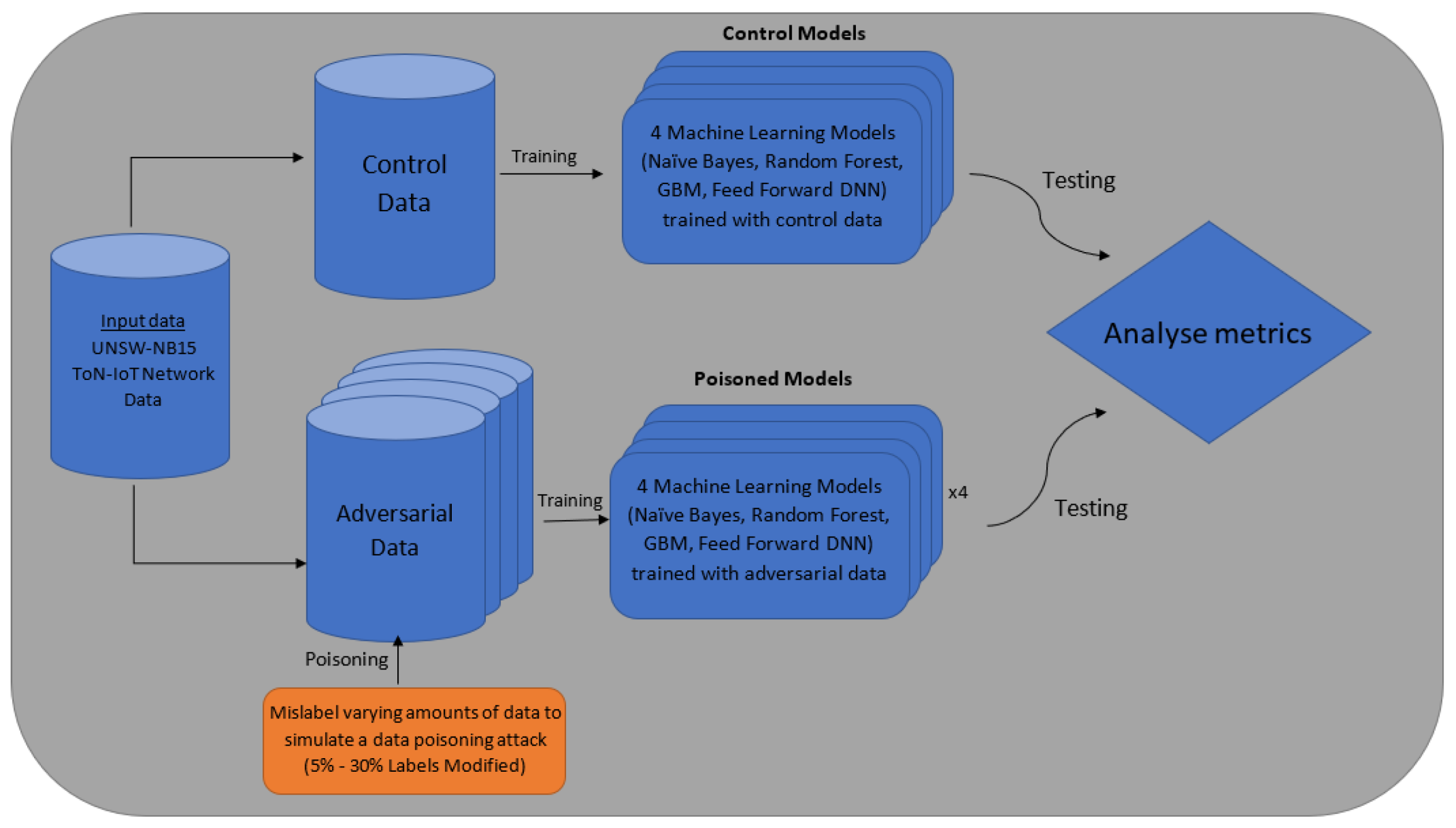
• We developed a label modification function that simulates data poisoning attacks by modifying the normal classes of the ToN_IoT and UNSW NB-15 datasets.
• We evaluated each of the ML models’ performances before and after data poisoning attacks, enabling discussion of the potential risks and advantages of these models.

The remainder of this paper is structured as follows. Section 2 provides a summary of related background and prior studies. Section 3 describes the methodology of the study, outlining how the data should be processed, poisoned, and modelled in order to derive suitable data for comparisons and discussion. In Section 4, the specifics of the experimental design are discussed to allow for replication. Finally, in Section 5, the experimental results are analysed and discussed before concluding the paper in Section 6.

2. Background and Related work

This section provides a review of the topic background and related studies, particularly those focused on adversarial machine learning, adversarial examples, and data poisoning.

2.1. The Unique Nature of IoT

In many respects, IoT represents the future of ubiquitous computing. Strong device integration promises increased efficiency, increased convenience, and new features only available with the integration of software, hardware, and cloud-based systems [14,15]. IoT itself is built on several other emerging technologies: cloud computing, the proliferation of low-powered, low-cost processors, wireless networking, increased Internet connectivity, and mobile computing [16].

IoT ecosystems include three main components: small devices that contain sensors and actuators, network communications, and cloud-based storage and processors [17]. The consumer-facing devices are the cyber-physical component, comprised of processors, sensors, and/or actuators. These devices utilise minimal processing, are often low-cost, and are designed to rely on network connectivity. In many cases, it is difficult or impossible to update or upgrade these systems once implemented, and many will not work correctly without the other ecosystem components [15]. The communications protocols used in IoT deployments are dependent on the individual system, and may include Zigbee, Bluetooth LE, Bluetooth, or one of several other bespoke or niche standards [18]. Ultimately, all communication is routed through the Internet.

The cloud-based components of an IoT ecosystem contain the data storage, processors, and the command and control to make decisions and influence other aspects of the ecosystem. Such components are less open to external scrutiny; they are far removed, not subject to reverse-engineering, regularly updated, and unique to each manufacturer or provider. They are also closely guarded, as the cloud deployments conduct processing, and as such, contain the majority of features. As such, there is little understanding of the ML models used, protections made, and safeguards in place.

The addition of IoT platforms to home, corporate, and industrial networks is considered inevitable [19,20]. However, the inclusion of one or more IoT ecosystems also changes network traffic in several ways. It changes usage patterns, volumes, protocols used, and destinations. From a cyber-security perspective, each of these increases the difficulty of locating a cyber-attack across a network [21]. The nature of IoT is unique, and differs from other applications from several perspectives; from a network perspective, from a cyber-security perspective [22], and also from a machine learning perspective.

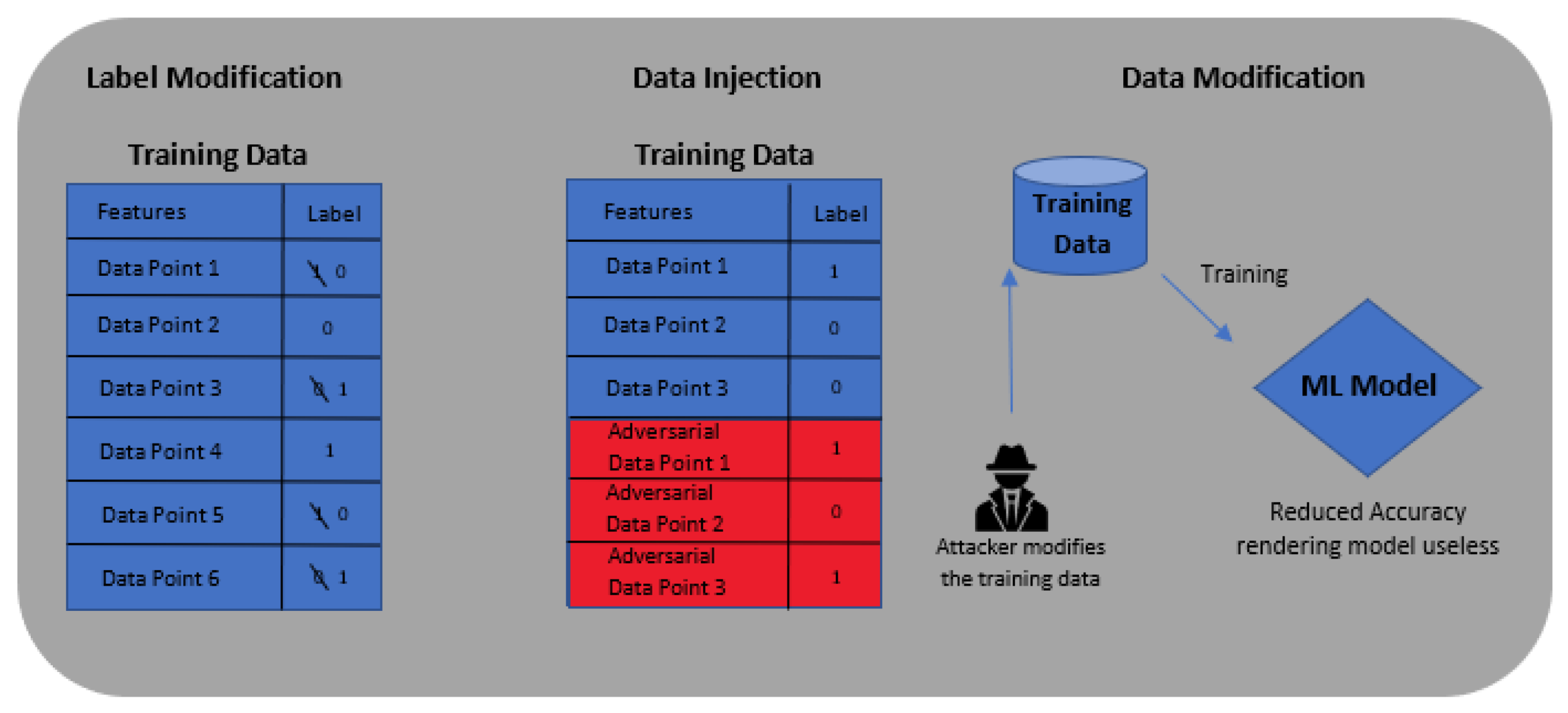
2.2. Adversarial Machine Learning

Machine learning algorithms meet the requirements of complex systems to gain insights and make decisions from large-scale data. As these algorithms are used increasingly in business, military, and other real-world use-cases, the requirements for security of these systems and privacy of their data become proportionally more important. Within cyber-security systems, machine learning algorithms are considered to be the weakest link because their nature of constant evolution, and the ability of sophisticated adversaries to manipulate their behaviours to exploit models [6]. There are several ways in which an adversary can violate a machine learning model [23]. Integrity attacks allow “adversarial inputs” to be classified as normal data and cause the filter to pass through a false negative rate. Availability attacks exploit a ML model and cause numerous incorrect classifications, such as a denial of service attack. Privacy attacks allow adversaries to infer confidential information about the learning process or the system’s users [23].

ML models applied to real-world systems must deal with dynamically changing data patterns and a wide variety of inputs, to the extent that it is highly improbable that every situation is captured in the training data [24]. Areas wherein a ML model is vulnerable are known as “adversarial regions” [25], which are near the decision boundary. This indicates that training data have not covered the entire feature space, which allows adversaries to apply trial and error or reverse engineering to find “adversarial samples”. These can be used to fool the model and enable the data inputs to be misclassified, thereby compromising a classifier and the integrity of its system. These attacks are exploratory and commonly known as evasion attacks [23]. Thomas et al. [26] utilised a generative adversarial network (GAN) dubbed Malware-GAN to generate adversarial malware examples against a black-box classifier. Once the attack was carried out, the true positive rate (TPR) fell to almost 0, indicating that the classifier was unable to detect the malware, rendering it useless. In situations wherein an attacker has access to the training data, an attack is considered causative, and poisoning attacks can be employed [23]. However, this GAN model can not identify all types of adversarial examples and requires extensive computational resources.

2.3. Data Poisoning Attacks and Defences

Non-stationary ML models trained on user-provided data are vulnerable to data poisoning attacks, whereby malicious users would inject false training data to corrupt the learning process, subsequently degrading the accuracy of the classifier and the integrity of the overall system [9]. The attacks give way to further exploits, including evasion attacks, backdoor attacks, or neural network Trojans. When attacking a model using data poisoning, adversaries have three broad strategies available to them, depending on their level of access to the data and learning process. This is shown in Figure 1. First, label modification is a technique used when an adversary is constricted and cannot inject their inputs but can modify the labels of the existing data in supervised learning datasets [10]. Second, data injection attacks do not have access to current training data or the learning algorithm but can inject their own “adversarial inputs” into the new training set [11]. Third, data modification attacks can occur when an adversary has no access to the learning algorithm but has full access to training data [27]; the data can be poisoned by modifying the data before being used to train the model.

There are two defences against data poisoning attacks outlined in the literature [28]: outlier sanitisation and reject on negative impact (RONI). Outlier sanitisation defences [9] identify data points that are significantly different from historical training data and reject them. The challenge with outlier sanitisation is to optimise the threshold to consider how far outside the “local group” a data point must be to be considered an outlier. If this threshold is too far, the model will be susceptible to poisoning, but too close and the model could be under-fitted and ineffective. Aside from managing this threshold, outlier sanitisation has other flaws; poisoned data points may be carefully placed near the threshold to move the decision boundary slowly over many iterations. This attack, known as the boiling frog attack [23], has shown to significantly increase evasion success after weeks of incremental poisoning. The RONI technique, first proposed by Barreno et al. [29], measured the effect of classifier accuracy after adding each training input and rejecting inputs which had a significant negative impact on the accuracy. To determine which training points are malicious, a control classifier is trained on a base set of inputs, which then adds new training data to the set to train a second classifier. The two classifiers are tested, and the accuracy of the latter is compared against the first control classifier. If the accuracy of the second classifier is significantly negatively impacted by the new data, the data are rejected from the training set. RONI is far less susceptible to the boiling frog attack, but is complex to configure and operate.

2.4. Adversarial Modelling

Threat models are a method used to optimise ML models, to find where a system is vulnerable, based on the knowledge and capabilities of the attackers. Thomas et al. [26] developed three threat models and launched attack techniques as listed below.

• Perfect knowledge adversary: This adversary is aware of the model’s parameters and detection techniques used to secure the model. Through the use of an adaptive white-box attack, the attacker can evade the ML model and the detector [26]. Using the assumption that the attacker has full knowledge of the ML algorithm, its parameters, hyperparameters, and the underlying architecture, their aim would be to develop an appropriate loss function to create adversarial examples capable of effectively evading the ML classifier.
• Limited knowledge adversary: This adversary does not have access to the detector implemented nor the training data; however, it does have knowledge of the detection scheme used to secure the model and the training algorithm. As the attacker is unaware of the underlying architecture and the parameters, a black-box attack must be used [26]. The attacker’s aim would be to create a training set similar in size and quality to the original, to train a substitute model.
• Zero-knowledge adversary: This adversary does not have access to the original detector, nor knowledge of the ML algorithm used. This threat model is very weak, as the attacker is not aware of the defences used to secure the underlying model. The attacker would use a black-box attack such as Carlini and Wagner’s [30] attack to try defeat the ML model. If the attack fails and the adversarial sample is detected, it can be said that the two previous attack models would also fail to defeat the detection mechanism [26].

2.5. Existing Literature

There have been several studies into data poisoning within the broader field of adversarial machine learning. For instance, Rubinstein et al. [31] demonstrated that anomaly detection systems trained on network traffic poisoned by injecting chaff traffic, increased the false-negative rate to 28% in single training period poisoning, and greater than 70% over multi-training period poisoning. They proposed a network-wide anomaly detection method, antidote, which was less sensitive to outliers and can reject poisonous training data. Barreno et al. [29] proposed the RONI defence technique and demonstrated its effectiveness; however, it was limited in only being trained and tested on spam email data. It is noted that the RONI technique can potentially remove useful information from the training data; however, it is an area that requires further research.

Siciu et al. [32] modelled adversaries’ knowledge, approaching the shortcoming that a lot of research had suffered to date; there was an assumption that an attacker had unrealistic knowledge and control over the data and learning process. The authors in [9] proposed a poisoning attack that was able to bypass existing defences easily and was tested against a variety of theoretical adversaries. Yang et al. [33] proposed a poisoning attack, utilising a generative method to increase the generation of poisoned data by leveraging the model’s gradient. A countermeasure was also introduced to detect poisoned data through the analysis of the loss during training stage. Despite the surge in the study and use of deep neural network (DNNs) in academic literature, there has not been substantial research into poisoning attacks on DNNs. Steinhardt et al. [9] showed that, even with a strong defence, an attack on a DNN with a 3% modification of the training set resulted in an 11% loss in classifier accuracy. In our study, we explore how data poisoning attacks could violate the performances of ML algorithms and to what rates of data modification the algorithms can be trusted.

3. Proposed Methodology

This section details the proposed methodology of this study. This includes a description of the data poisoning process, an outline of each of the ML models studied, their training process, datasets used, and metrics implemented to evaluate each model. As seen in Figure 2, the control models were trained on the original datasets to gain an understanding of the performance of each model within a non-adversarial environment. The models were also trained on the four sets of adversarial data (i.e., label modification), that were manipulated during the data poisoning stage, at increasing rates (5%, 10%, 20%, 30%). The models were then compared based on the evaluation metrics of accuracy, precision, false positive rate, and detection rate.

3.1. Data Poisoning Process

The training datasets (D^S) were structured so that most of the normal traffic observations were grouped to simulate the data poisoning attack on the data classes. The normal observations were randomised to ensure there was not a bias towards poisoning a large proportion of only normal data or only attack data. Once the data were randomised, they were parsed by a Python script which would calculate the number of labels to flip (L_poison) based on the percentage designated. As described in Algorithm 1, the data was poisoned at four rates (r_poison) (5%, 10%, 20%, 30%) to demonstrate the effects of increasing data poisoning on the classifiers. The required labels were flipped within the randomised datasets, and the poisoned datasets (D^P) were used to train the ML models, which are detailed below.

Algorithm 1: Data poisoning process using label modification.

3.2. Machine Learning Models

3.2.1. Gradient Boosting Machine

Boosting is a procedure that combines many weak or “simple” learners, those whose performances are slightly better than random guessing, to produce a more robust committee whose performance is greater than the sum of its parts. If each of these learners is trained on the same dataset, there will be little, if any difference between them, so a boosting algorithm, to improve it’s learners, must manipulate the data it feeds into each of the separate learners [34]. As the data are incrementally changed, weak learners are trained sequentially to produce a series of decision trees, or decision stumps, to provide an overall more robust organisation of weak classifier models [35].

The regression tree boosting model learns slowly; instead of training a broader decision tree for the whole dataset, likely overfitting it, the new trees learn from the residuals of the current model. As each tree is added to the model, the residuals are updated, allowing the model to improve in areas it is lacking. Each new tree strongly depends on the previous trees in the model. Algorithm 2 presents the steps of the regression tree boosting model [35].

Algorithm 2: Algorithm of regression tree boosting.

3.2.2. Random Forest

A random forest is built from multiple decision tree classifiers. A decision tree classifier is a flowchart-like structure made of decision nodes and leaf nodes. The decision nodes compute an outcome which determines the next sub-tree, where the data will move to. Leaf nodes are the final nodes in the branch and are associated with a class, which will be allocated to the data at test time [36]. Decision trees are easy to visualise and interpret, and for this, there are white box machine learning algorithms. As the data traverse through the decision tree, they are broken down into smaller subsets based on the features in the decision nodes, until they reach leaf nodes and classifications are made. If a tree is allowed unlimited depth during training, it will eventually build a structure that can correctly classify all training data. While this may seem beneficial, the tree will be wildly overfitted and will not be able to effectively classify new data correctly.

An alternative to this is to build forests, a collection of decision tree classifiers that operate together to classify the data. To be classified as a random forest, each tree is built with a random subset of the training data through a process known as bootstrapping. In this process, the training samples are drawn with replacement to build random training subsets. Each tree also utilises a random selection of the features within the decision nodes of the tree, commonly a set equal to the square root of all possible features. When testing, each tree is shown the test data point and classifies that point. The overall classification of the random forest is the average of all trees classifications. Relying on the average of multiple different classifiers creates a model that has an overall lower variance and bias.

The committee assembles the prediction algorithm f as a collection of the individual trees in the ensemble h₁(x), h₂(x),…, h_j(x) to build the “ensemble predictor” f(x) [36]. In classification, f(x) is the most frequently predicted class, as voted by each of the individual trees [36]:

$$f\left(x\right)=argmax\sum _{j=1}^{J}I\left(y=h_j\left(x\right)\right)$$

(1)

where I (y = h_j(x)) = 1 if y = h_j(x) and 0 otherwise.

3.2.3. Naive Bayes

Naive Bayes is a family of probabilistic machine learning models based on the Bayes theorem [37]:

$$P\left(A|B\right)=\frac{P\left(B|A\right)P\left(A\right)}{P\left(B\right)}$$

(2)

where P(A) is the probability of A, P(B) is the probability of B, and P(A|B) is the probability of A given B.

The Bayes theorem finds the probability of an event occurring given the likelihood of another event that has already occurred. Given that the denominator does not rely on the classes, and that naive Bayes assumes all features of the data are independent and contribute individually to the classification, we can rewrite the formula as:

$$P\left(A|B\right)=P\left(A\right)\prod _{i=1}^{n}P\left(B_i|A\right)$$

(3)

where $B=\left(b_1,\dots ,b_n\right)$ representing some n features.

Combining this model with a decision rule generates a naive Bayes classifier. There are multiple types of naive Bayes model, such as the Gaussian naive Bayes, Bernoulli naive Bayes, and multinomial naive Bayes. The advantages of naive is that it is robust to isolated noise and outliers as it is not sensitive to irrelevant features. Naive Bayes can be used for binary or multi-class data problems, is highly scalable, and does not require an extensive training set to be effective. The disadvantage of naive Bayes is that it assumes mutual independence between features, whereas this is unlikely to occur within a realistic dataset. Moreover, as a simplistic statistical classifier [2], it may be sensitive to poisoning attacks that strongly impact the data, distorting the probabilities used for predictions.

3.2.4. Feed Forward Deep Learning

The feed forward deep neural network, also known as a multilayer perceptron (MLP), is the foundation of deep learning models [38]. The model is referred to as “feed forward”, as information passes through the function and there are no feedback connections in which the outputs would be fed back into the model. Neural networks are comprised of many layers of neurons, also known as perceptrons. The first layer is referred to as the input layer, as data are fed into these neurons. The final layer is the output layer, in which the model will predict a class for the specified input data, based on the learning algorithm. The layers in between are known as hidden layers, as the behaviour of the neurons is not specified by the input data and the training algorithm will decide how to most effectively use these layers to produce the desired output [38].

Each neuron in the hidden layers receives several inputs and produces a single output. Each input x₁, x₂, x₃ has a corresponding weight w₁, w₂, w₃ expressing the respective importance of each of the inputs to the output. The output of the neuron is determined by weighted sum, as shown in [38]:

$$output=\{\begin{array}{c}0\mathrm{if}\sum _i^{}{w}_i{x}_i\le threshold\\ 1\mathrm{if}\sum _i^{}{w}_i{x}_i>threshold\end{array}$$

(4)

This binary piecewise function is known as “an activation function”, used to determine whether a neuron will “fire” or not. Many activation functions are used throughout the field of deep learning, such as a sigmoid function, a binary step function, and a rectified linear unit (ReLU) function, each with their own advantages and disadvantages. The overall goal of the training algorithm is to find a set of weights and biases (thresholds) that allows the network to accurately classify new input data [39]. The cost function determines the difference between the outputs of the model and the correct labels of the input data. The basic quadratic cost function is defined as:

$$C\left(w,b\right)\equiv \frac{1}{2n}\sum _x^{}{\parallel y\left(x\right)-a\parallel }^2$$

(5)

where n is the number of inputs, y(x) is the correct label of the input data, and a is the output of the model when x is the input [38].

Using gradient descent, the cost function can be minimised, thereby finding the weights and biases that approximate some functions f that can map the input x onto the correct output label y(x).

3.3. Training Phase of ML Algorithms

Each ML algorithm (gradient boosted machine (GBM), random forest (RF), naive Bayes (NB), and feed-forward deep neural network (FFDNN)) was trained five times, covering the varying levels of poisoning in the input data (D^P₅, D^P₁₀, D^P₂₀, D^P₃₀). The parameters were unchanged between training iterations. The pre-processed input data (D^S, D^P) are provided to the models to train on and allows us to track differences in the models based on the independent variable, percentage of data poisoned (r_poison).

The ML models (M) were trained and validated using the H2O API and the R programming language, allowing for further analysis of the training and validation metrics and comparisons of models. As presented in Algorithm 3, the models were trained using five cases: Correctly labelled normal and attack data (D^S), as the control models (M^normal). The normal and attack data, along with a percentage of the training data mislabelled (D^P), and the poisoned models (M^Poisoned), were employed to determine the variations between the five cases and examine the robustness of the models.

Algorithm 3: ML algorithm training process.

3.4. Validation Process of ML Algorithms

The models built in the training phase were validated using k-fold cross validation in order to ensure there was no bias towards dominant classes. K-fold cross validation is a method used to test a model, determining the model’s performance over the entire dataset. The method splits the dataset into k equal groups, or folds [35]. One of the groups is designated as the validation set, while the k-1 additional groups are used to fit the model. The mean squared error (MSE) is calculated on the validation set. This process is repeated k times, with a different set used as the validation set each iteration. The method results in k estimates of the test error [34]. The k-fold cross validation error estimate is explained in [35], calculated as:

$$C{V}_{\left(k\right)}=\frac{1}{k}\sum _{i=1}^{k}MS{E}_i$$

(6)

4. Experimental Design

4.1. Data Sets

The datasets used to evaluate the models were the UNSW-NB15 Network Data [12] and the ToN-IoT Network Data [13]. Both datasets contain a wide variety of contemporary normal and abnormal network observations, which allowed practical training of all models in order to mimic a model deployed as part of a more extensive network security application. Both these datasets contain a known ground truth. The UNSW-NB15 dataset contains approximately 100 Gigabytes of network packets across 2,540,044 vectors recorded in four CSV files [12]. The data include normal and a variety of attack vectors. (Fuzzers, analysis, backdoors, DoS, exploits, generic, reconnaissance, shellcode, and worms). Partitions of this dataset have been configured as training and testing sets for use in machine learning. The training set consisted of 175,341 network packet vectors, and the test set contained 82,332 vectors. Each vector comprised 42 features and the class label of either normal (0) or attack (1).

The ToN-IoT Network dataset consists of 56 Gigabytes of raw network data. The data were processed and compiled into one CSV file for training and validating machine learning models [13]. The dataset consists of 461,043 network packet vectors. Each vector comprises 43 features and the class label of either normal or attack data. Before training, the ToN-IoT dataset was split into training and testing sets, 70% for training and 30% for testing, reducing the likelihood of overfitting and allowing for a comprehensive measure of the model’s performance throughout the whole dataset.

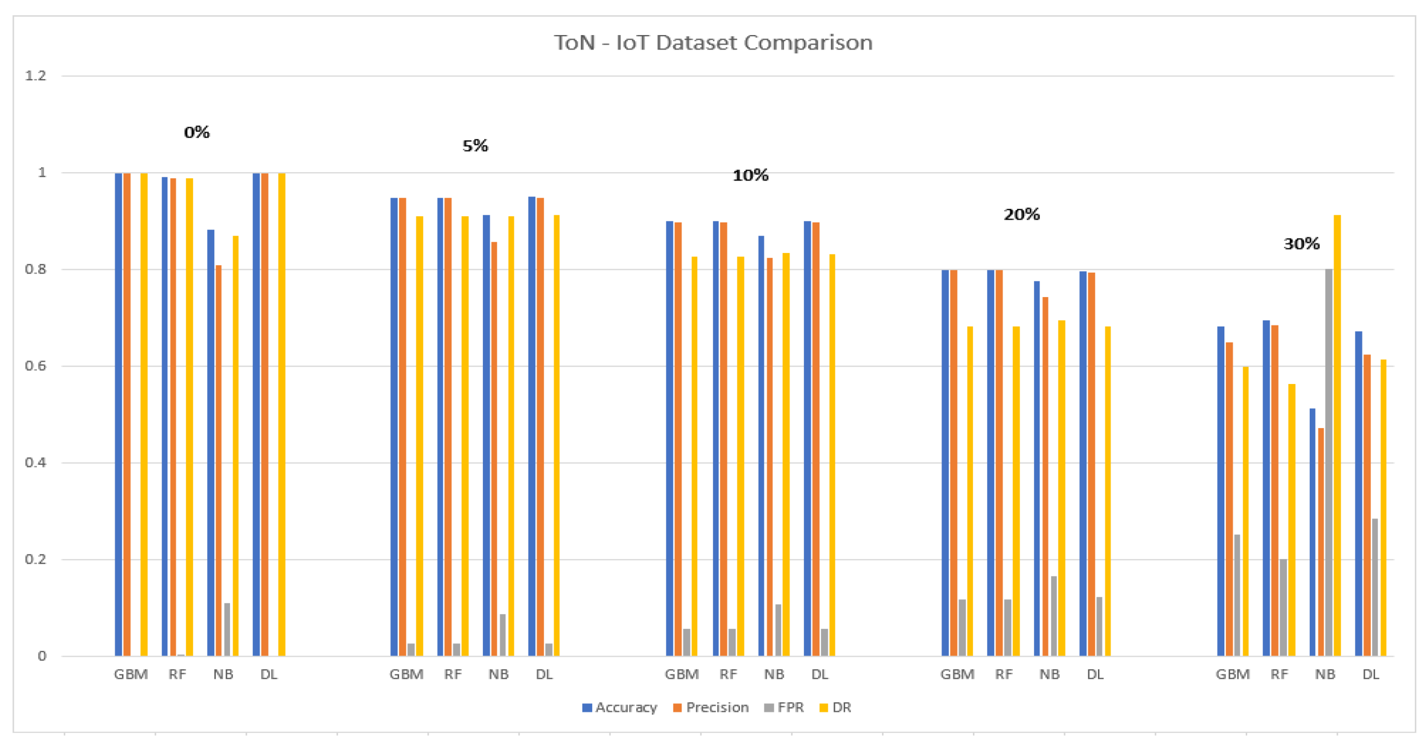
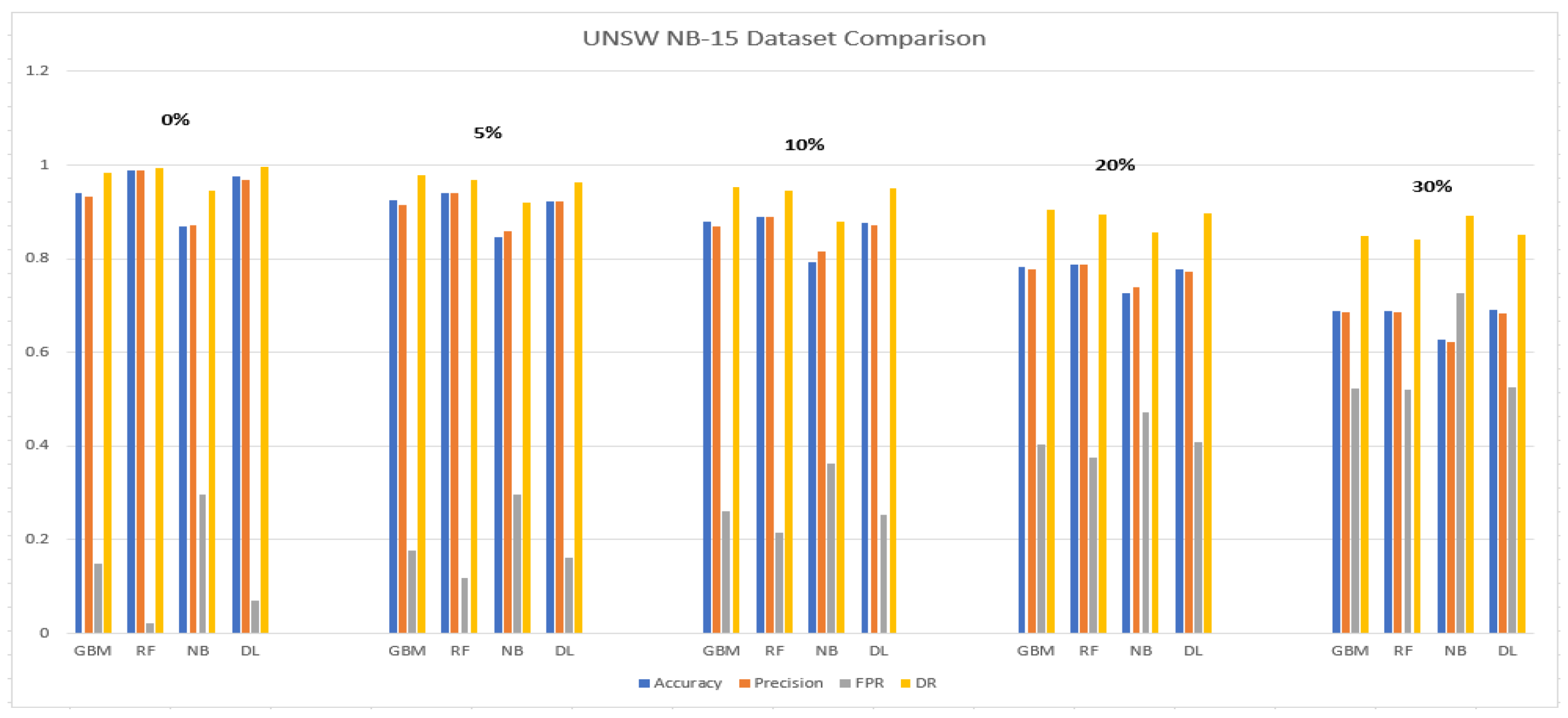
4.2. Evaluation Metrics

The models were trained on both datasets and with various levels of poisoned training data in order to evaluate their performances, in terms of accuracy, precision, false positive rate, and detection rate. These metrics were calculated from the four classifications of true positive (TP), true negative (TN), false positive (FP), and false negative (FN). TP and TN are the numbers of correctly classified legitimate and attack vectors, respectively, whilst FP and FN are the incorrectly classified legitimate and attack vectors, respectively [3].

• Accuracy is the proportion of the test data that was correctly classified by the model:

  $$Accuracy=\frac{TP+TN}{TP+TN+FP+FN}$$

  (7)
• Precision is the proportion of vectors classified as attacks that are relevant:

  $$Precision=\frac{TP}{TP+FP}$$

  (8)
• False positive rate (FPR) is the proportion of incorrectly classified attack vectors:

  $$FPR=\frac{FP}{FP+TN}$$

  (9)
• Detection rate (DR), also known as true positive rate (TPR), is the proportion of correctly classified attack vectors, for which a result of one (1) indicates that the model detected all attack vectors in the test data:

  $$DR=\frac{TP}{TP+FN}$$

  (10)

The models were developed using the “R programming language” on Windows 10 Version 1809 with 16 GB RAM and an Intel i7 CPU processor. The models and their data were stored and analysed using H2O API. More information about H2O can be found at [40]. All code used in this study can be found at [41]. The parameters of the models can be seen in

Table 1. Model parameters.

Model Parameters
Gradient Boosted Machine		Random Forest		Naive Bayes		Feed-Forward Deep Neural Network
Trees	100	Trees	150	Laplace Smoothing Parameter	3	Hidden Layer Size	[15,15]
Max Depth	5	Stopping Rounds	2	Max after balance size	5	Epochs	10
Min Rows	2	Seed	10000	Minimum sdev	0.01
Learning Rate	0.01	Distribution	Multinomial

. Throughout the training, all parameters remained constant to accurately capture the differences between the poisoned datasets.

5. Experimental Results

5.1. Original Data (0% Poisoning)

5.1.1. ToN-IoT Dataset

Using the ToN IoT dataset, we observed over 99% accuracy for all models besides the naive Bayes model, with an 88.4% accuracy rate, and an increased false positive rate of 10.9% in comparison to the 0.02–0.5% false positive rate observed in the other three models, as shown in Figure 3. The highest performing model was the gradient boosted machine, with an accuracy of 99.985%, only 0.005% more accurate than what was observed in the feed forward deep learning model. However, the deep learning model had a marginally superior precision of 99.972% when compared to the gradient boosted machine, with a precision of 99.965%. Both models display impressive statistics in a sanitised environment, with no adversarial data present.

5.1.2. UNSW NB-15 Dataset

When trained on the UNSW NB-15 dataset, the models performed significantly lower in all metrics, with all models indicating a 2–5% drop in accuracy when compared to the models trained on the ToN_IoT dataset, as depicted in Figure 4. Due to the model parameters remaining constant across all training periods, the set parameters have been favourable to the ToN_IoT data, leading to the underperformance of the UNSW NB-15 models. The highest performing model was the random forest model, with accuracy and precision of 98.9%, FPR of 2%, and DR of 99.4%. This model displays an increased performance of 1–2% in all metrics over the next highest performing model (feed forward deep learning). However, the deep learning model’s detection rate marginally outperformed the random forest model, with a rate of 99.5% in comparison to the random forest’s 99.4%.

5.2. 5% Poisoned Data

5.2.1. ToN-IoT Dataset

When trained on a dataset with 5% mislabelled training data, all models besides the naive Bayes classifier show a 5% drop in accuracy, as expected. The naive Bayes classifier’s accuracy increased from 88.4% when trained on the poisoned data, to 91.3% when trained on 5% poisoned data. The naive Bayes model also displayed a 4% increase in precision and detection rate and a 2% decrease in false positive rate. All models had a detection rate of approximately 91%, illustrating that even at 5% poisoning, these models are already showing a significant loss of integrity, with 9% of attack vectors going undetected. The highest performing model was the deep learning model, with an accuracy of 95.1%, precision of 94.8%, FPR of 2.8%, and DR of 91.3%—only marginally outperforming the gradient boosting machine and random forest by 0.1–0.3% in all metrics. It is clear that all three models are equally impacted by the poisoning at this stage, with significantly reduced detection rates of 91%, at just 5% poisoning.

5.2.2. UNSW NB-15 Dataset

The models trained on the UNSW NB-15 dataset with 5% mislabelled data showed a decreased accuracy when compared to the ToN-IoT models. The naive Bayes classifier showed a 2% drop in accuracy to 84.6%, and the other three models’ accuracies decreased by approximately 5%, equally impacted as the ToN-IoT models. The highest performing model was the random forest, with an accuracy of 93.9%, a 1.4% increase over the gradient boosted machine, which had an accuracy of 92.5%. The random forest model boasted a 1.8% increase in precision over the deep learning model and 4% lower false positive rate when compared to the next closest model. It did, however, display a 0.8% lower detection rate than the gradient boosted machine, with a DR of 96.9% compared to 97.7%, respectively.

5.3. 10% Poisoned Data

5.3.1. ToN-IoT Dataset

When trained on 10% mislabelled data, the models showed a 10% loss of accuracy and precision, with an accuracy of 89.9–90% and precision of 89.9%, except the naive Bayes classifier, which had an accuracy of 86.9%—a 4.4% decrease when compared to the model trained on 5% poisoned data, and a 2% decrease when compared to the model trained on the original sanitised data. The gradient boosted machine, random forest and deep learning models all performed similarly, with the deep learning model having a marginally higher accuracy of 90.0% in comparison to 89.9% for the other two models. The naive Bayes classifier had the highest detection rate, at 83.4%; however, it severely underperformed compared to the other three models in all alternative metrics.

5.3.2. UNSW NB-15 Dataset

The models trained on the UNSW NB-15 dataset with 10% mislabelled data showed similar results to the models trained on the poisoned ToN IoT data, but underperformed by 1–2% in most metrics. Accuracy and precision were impacted by 11–12% for all models except the naive Bayes classifier, with an accuracy of 79.3% and precision of 81.5%. All models besides the naive Bayes classifier showed a DR of 94–95% which is significantly higher than for the models trained on the ToN-IoT dataset. Coupled with increased FPRs, this is an early sign of classifier integrity loss, as the models begin to classify a higher proportion of test data as attack vectors. The highest performing model was the random forest, with an accuracy of 88.9% and precision of 88.9%. The random forest significantly outperformed the next closest model with an FPR of 21.4% when compared to the feed forward deep learning model, with an FPR of 25.4%. The gradient boosted machine model outperformed the random forest with a detection rate of 95.4% compared to the 94.5% observed by the random forest model.

5.4. 20% Poisoned Data

5.4.1. ToN-IoT Dataset

When trained on 20% mislabelled data, all models except the naive Bayes classifier showed approximately a 20% drop in accuracy and precision, to 79.7–79.9% and 79.3–79.9% respectively. The naive Bayes classifier underperformed compared to the other models, with an accuracy, precision, and false positive rate of 77.7%, 74.5%, and 16.6% respectively. However, as observed in the 10% mislabelled data, the naive Bayes classifier had the highest detection rate of 69.6%, compared to the next highest, that being the gradient boosted machine with a DR of 68.3%. The highest performing models were the gradient boosted machine and random forest, which had almost identical metrics, and only marginally outperformed the deep learning model in all metrics. At a rate of 20% data poisoning, the models were severely compromised, with detection rates of 69%. This is unacceptable for any model deployed to a real-world environment, with 21% of all attack vectors going undetected.

5.4.2. UNSW NB-15 Dataset

The models trained on the UNSW NB-15 dataset with 20% mislabelled data showed similar results to the models trained on the poisoned ToN IoT data, although underperformed by 1–2% in most metrics. Accuracy and precision were impacted by 21–22%, except for the naive Bayes classifier, with an accuracy of 72.8% and precision of 73.9%. All models display a detection rate of 85–90%, which is significantly higher than the models trained on the ToN-IoT dataset. The highest performing model was the random forest, with an accuracy of 78.8% and precision of 78.7%. The random forest significantly outperformed the next closest model with an FPR of 37.5% when compared to the gradient boosted machine, with an FPR of 40.4%. The gradient boosted machine model outperformed the random forest with a detection rate of 90.3% compared to the 89.3% observed by the random forest model.

5.5. 30% Poisoned Data

5.5.1. ToN-IoT Dataset

When trained on 30% mislabelled data, all models except the naive Bayes classifier showed decreased in accuracy approximately proportional to the mislabelled data in the training set. The metric data sees a split here, with the deep learning model becoming more heavily impacted when compared to the gradient boosted machine and random forest models. The naive Bayes classifier continued to underperform the other three models significantly, but at this point saw a drop in accuracy to 51.2% and precision to 47.1%, and a had a false positive rate of 80.1%. As seen in Figure 3, the naive Bayes classifier saw a significant increase in detection rate to 91.2%. This rapid increase showed corruption in the model’s decision rule, predicting all vectors as attack vectors, hence the substantial increase in both FPR and DR.

The highest performing model was the random forest model, with an accuracy of 69.5%, precision of 68.7%, FPR of 20.2%, and DR of 56.5%. At this level of data poisoning, the models were unable to accurately classify the test data, with detection rates ranging from 56.4–61.4% for all models except the naive Bayes classifier, which was discussed previously. The random forest model stands out above the others for its superior FPR of 20.2% when compared to the next closest, that being the gradient boosted machine with an FPR of 25.2%.

5.5.2. UNSW NB-15 Dataset

The models trained on the UNSW NB-15 dataset with 30% mislabelled data showed similar accuracy and precision loss to the models trained on the poisoned ToN IoT data, besides the naive Bayes classifier, which outperformed the model trained on the ToN_IoT dataset in all metrics other than DR. As per the previous models trained on the UNSW NB-15 dataset, all models had significantly increased FPR, indicating a severe loss in classifier integrity, leading to FPRs of 72.7% for the naive Bayes classifier and 51–52% for the other three models.

The highest performing model at this rate of poisoning was the deep learning model, with an accuracy of 68.9%, precision of 68.3%, FPR of 52.4%, and DR of 85.1%. As stated previously, all models at this stage of poisoning are severely corrupted and are unable to classify large proportions of the test data correctly. Notably, the gradient boosting machine and random forest models performed similarly at this rate of poisoning.

5.6. Discussion

The data suggest a proportionate correlation between the rate of data poisoning and the impact on the model’s performance. This is best highlighted in the models trained on the ToN_IoT dataset; between 0% and 20%, the more reliable models (gradient boosting machine, random forest, and deep learning models) showed a drop in accuracy and precision directly proportionate to the percentage of poisoned data in the training set. The results confirm that these models are not robust to any level of data poisoning; as at 5% poisoning, the detection rates of all models dropped by 3–9%. At this rate, the ML model would be unfit to persist in online defences such as intrusion detection, so the attacker had successfully deteriorated the availability of the model.

Beyond 30% poisoned training data, all three machine learning models showed increased deterioration of DR, and a spike in FPR, indicating that 20% is the threshold in which the models are severely effected by the poisoning, as the deterioration of the model is no longer proportional to the rate of data poisoning. This is also seen in the results of the DL model.

The feed forward deep learning model at 30% began to underperform compared to the gradient boosting machine and random forest models, indicating that past 20% poisoning, deep learning models became more severely affected by the data poisoning than other models in the study. This suggests that deep learning models are less robust to data poisoning; however, at this rate of data poisoning, all models are unable to classify large proportions of the data correctly and are considered unusable. A model performing at this rate in a live scenario would be taken offline and retrained.

Throughout the results, the random forest model consistently outperformed the other three models, especially at higher rates of poisoning. Between 0–20% poisoning, the gradient boosting machine, random forest, and deep learning models performed similarly, generally remaining within 1% for all metrics. This indicates that for lower levels of poisoning, these three models can be used interchangeably with similar results when applied to a live system. However, upon crossing the 20% poisoning threshold, the random forest model outperformed the other models significantly, featuring a 5% lower FPR than the gradient boosting machine and 8% lower FPR than the deep learning model. The naive Bayes classifier consistently underperformed compared to the other three models throughout the experiment.

This is unsurprising, as a simplistic statistical classifier, it is unsuitable for training on network data, and is heavily impacted by the poisoned data. As the rate of poisoned training data is increased, the probabilities used by the classifier to predict test data would be increasingly distorted, and as seen in the data, make it less likely to correctly predict the correct class of the data. A primary limitation of the study is the underperformance of the models trained on the UNSW NB-15 dataset; this can be attributed to the parameters used throughout the study remaining unchanged across each training iteration. To increase the success of further research, it is recommended that models trained on multiple datasets be prepared using parameters tuned to that data, in order to more accurately understand the initial performance of the models using said data.

The proposed scheme attempted to practically evaluate the impact of data poisoning attacks against the training phase. Based on building shallow and deep learning models using two datasets, the results demonstrated that increasing the number of manipulated labels led to reduced accuracy and increased false positive rates with different cross validation settings (i.e., k = 10 for the four machine learning models using the two datasets). From the results, we can claim that by using both datasets with up to a 20% data poisoning rate, the ML models’ accuracy remained proportional to the rate of poisoned data. However, after increasing this rate, the models began to degrade considerably. The main advantages of this scheme are that: (1) we practically identified how the data poisoning attacks impact the accuracy of ML models; (2) we evaluated different data settings with heterogeneous data sources (i.e., conventional network traffic, and IoT network traffic), revealing the trustworthiness of various ML models. In the future we aim to use GPU cards, as the ML models will be developed much faster than using CPU resources; and dynamically configure parameters of ML models, so we can ensure the highest performances in terms of accuracy, false positive rate, and detection rate.

6. Conclusions

This paper has discussed the effects of data poisoning attacks, specifically label modification, on four machine learning models, in a effort to understand the innate robustness of each model and study the impacts of increasing rates of data poisoning. The models of gradient boosting machine, random forest, naive Bayes, and feed forward deep learning were trained on the two network datasets of UNSW NB-15 and ToN_IoT, and four poisoned sets. The models were evaluated against four metrics: accuracy, precision, false positive rate, and detection rate to determine the impacts to each model’s integrity suffered due to the poisoned training data. In the future, we will test the ML models with data poisoning defences to examine their effectiveness. This will allow for further evaluation of their robustness to poisoning attacks, and their suitability for use in online defence systems.

References

1. Al-Garadi, M.A.; Mohamed, A.; Al-Ali, A.; Du, X.; Ali, I.; Guizani, M. A survey of machine and deep learning methods for internet of things (IoT) security. IEEE Commun. Surv. Tutor. 2020. [Google Scholar] [CrossRef] [Green Version]
2. Rebala, G. An Introduction to Machine Learning; Springer: Cham, Switzerland, 2019. [Google Scholar]
3. Moustafa, N.; Choo, K.K.R.; Radwan, I.; Camtepe, S. Outlier Dirichlet mixture mechanism: Adversarial statistical learning for anomaly detection in the fog. IEEE Trans. Inf. Forensics Secur. 2019, 14, 1975–1987. [Google Scholar] [CrossRef]
4. Stellios, I.; Kotzanikolaou, P.; Psarakis, M.; Alcaraz, C.; Lopez, J. A Survey of IoT-Enabled Cyberattacks: Assessing Attack Paths to Critical Infrastructures and Services. IEEE Commun. Surv. Tutor. 2018, 20, 3453–3495. [Google Scholar] [CrossRef]
5. Vorobeychik, Y. Adversarial Machine Learning; Morgan & Claypool: San Rafael, CA, USA, 2018. [Google Scholar]
6. Duddu, V. A Survey of Adversarial Machine Learning in Cyber Warfare. Def. Sci. J. 2018, 68, 356–366. [Google Scholar] [CrossRef] [Green Version]
7. Moustafa, N.; Creech, G.; Slay, J. Anomaly detection system using beta mixture models and outlier detection. In Progress in Computing, Analytics and Networking; Springer: Berlin/Heidelberg, Germany, 2018; pp. 125–135. [Google Scholar]
8. Keshk, M.; Moustafa, N.; Sitnikova, E.; Creech, G. Privacy preservation intrusion detection technique for SCADA systems. In Proceedings of the 2017 Military Communications and Information Systems Conference (MilCIS), Canberra, Australia, 14–16 November 2017; pp. 1–6. [Google Scholar]
9. Steinhardt, J.; Koh, P.W.W.; Liang, P.S. Certified defenses for data poisoning attacks. In Advances in Neural Information Processing Systems; NIPS Proceedings: Long Beach, CA, USA, 2017; pp. 3517–3529. [Google Scholar]
10. Biggio, B.; Nelson, B.; Laskov, P. Poisoning attacks against support vector machines. arXiv 2012, arXiv:1206.6389. [Google Scholar]
11. Jagielski, M.; Oprea, A.; Biggio, B.; Liu, C.; Nita-Rotaru, C.; Li, B. Manipulating machine learning: Poisoning attacks and countermeasures for regression learning. In Proceedings of the 2018 IEEE Symposium on Security and Privacy (SP), San Francisco, CA, USA, 20–24 May 2018; pp. 19–35. [Google Scholar]
12. Moustafa, N.; Slay, J. UNSW-NB15: A comprehensive data set for network intrusion detection systems (UNSW-NB15 network data set). In Proceedings of the 2015 Military Communications and Information Systems Conference (MilCIS), Canberra, Australia, 10–12 November 2015; pp. 1–6. [Google Scholar] [CrossRef]
13. Moustafa, N. ToN_IoT Datasets. 2019. Available online: https://search.datacite.org/works/10.21227/fesz-dm97# (accessed on 7 August 2020).
14. Mazhelis, O.; Luoma, E.; Warma, H. Defining an internet-of-things ecosystem. In Internet of Things, Smart Spaces, and Next Generation Networking; Springer: Berlin/Heidelberg, Germany, 2012; pp. 1–14. [Google Scholar]
15. Firouzi, F.; Farahani, B.; Weinberger, M.; DePace, G.; Aliee, F.S. IoT Fundamentals: Definitions, Architectures, Challenges, and Promises. In Intelligent Internet of Things; Springer: Berlin/Heidelberg, Germany, 2020; pp. 3–50. [Google Scholar]
16. Firouzi, F.; Farahani, B. Architecting IoT Cloud. In Intelligent Internet of Things; Springer: Berlin/Heidelberg, Germany, 2020; pp. 173–241. [Google Scholar]
17. Bröring, A.; Schmid, S.; Schindhelm, C.K.; Khelil, A.; Käbisch, S.; Kramer, D.; Le Phuoc, D.; Mitic, J.; Anicic, D.; Teniente, E. Enabling IoT ecosystems through platform interoperability. IEEE Softw. 2017, 34, 54–61. [Google Scholar] [CrossRef] [Green Version]
18. Salman, T.; Jain, R. A survey of protocols and standards for internet of things. arXiv 2019, arXiv:1903.11549. [Google Scholar]
19. Ahlers, D.; Wienhofen, L.W.; Petersen, S.A.; Anvaari, M. A Smart City ecosystem enabling open innovation. In Proceedings of the International Conference on Innovations for Community Services, Wolfsburg, Germany, 24–26 June 2019; pp. 109–122. [Google Scholar]
20. Tange, K.; De Donno, M.; Fafoutis, X.; Dragoni, N. Towards a systematic survey of industrial IoT security requirements: Research method and quantitative analysis. In Proceedings of the Workshop on Fog Computing and the IoT, Montreal, QC, Canada, 15–18 April 2019; pp. 56–63. [Google Scholar]
21. Koroniotis, N.; Moustafa, N.; Sitnikova, E.; Turnbull, B. Towards the development of realistic botnet dataset in the internet of things for network forensic analytics: Bot-iot dataset. Future Gener. Comput. Syst. 2019, 100, 779–796. [Google Scholar] [CrossRef] [Green Version]
22. Hassija, V.; Chamola, V.; Saxena, V.; Jain, D.; Goyal, P.; Sikdar, B. A survey on IoT security: Application areas, security threats, and solution architectures. IEEE Access 2019, 7, 82721–82743. [Google Scholar] [CrossRef]
23. Huang, L.; Joseph, A.D.; Nelson, B.; Rubinstein, B.I.; Tygar, J.D. Adversarial machine learning. In Proceedings of the 4th ACM Workshop on SECURITY and Artificial Intelligence, Chicago, IL, USA, 21 October 2011; pp. 43–58. [Google Scholar]
24. Barreno, M.; Nelson, B.; Sears, R.; Joseph, A.D.; Tygar, J.D. Can machine learning be secure? In Proceedings of the 2006 ACM Symposium on Information, Computer and Communications Security, Taipei, Taiwan, 21–24 March 2006; pp. 16–25. [Google Scholar]
25. McDaniel, P.; Papernot, N.; Celik, Z.B. Machine learning in adversarial settings. IEEE Secur. Priv. 2016, 14, 68–72. [Google Scholar] [CrossRef]
26. Thomas, T.; Vijayaraghavan, A.P.; Emmanuel, S. Adversarial Machine Learning in Cybersecurity. In Machine Learning Approaches in Cyber Security Analytics; Thomas, T., Vijayaraghavan, A.P., Emmanuel, S., Eds.; Springer: Singapore, 2020; pp. 185–200. [Google Scholar] [CrossRef]
27. Biggio, B.; Rieck, K.; Ariu, D.; Wressnegger, C.; Corona, I.; Giacinto, G.; Roli, F. Poisoning behavioral malware clustering. In Proceedings of the 2014 Workshop on Artificial Intelligent and Security Workshop, Salamanca, Spain, 4–6 June 2014; pp. 27–36. [Google Scholar]
28. Nelson, B.; Barreno, M.; Chi, F.J.; Joseph, A.D.; Rubinstein, B.I.; Saini, U.; Sutton, C.; Tygar, J.; Xia, K. Misleading learners: Co-opting your spam filter. In Machine Learning in Cyber Trust; Springer: Berlin/Heidelberg, Germany, 2009; pp. 17–51. [Google Scholar]
29. Barreno, M.; Nelson, B.; Joseph, A.D.; Tygar, J.D. The security of machine learning. Mach. Learn. 2010, 81, 121–148. [Google Scholar] [CrossRef] [Green Version]
30. Carlini, N.; Wagner, D. Towards evaluating the robustness of neural networks. In Proceedings of the 2017 IEEE Symposium on Security and Privacy (SP), San Jose, CA, USA, 22–26 May 2017; pp. 39–57. [Google Scholar]
31. Rubinstein, B.I.; Nelson, B.; Huang, L.; Joseph, A.D.; Lau, S.h.; Rao, S.; Taft, N.; Tygar, J.D. Antidote: Understanding and defending against poisoning of anomaly detectors. In Proceedings of the 9th ACM SIGCOMM Conference on Internet Measurement, Chicago, IL, USA, 4–6 November 2009; pp. 1–14. [Google Scholar]
32. Shafahi, A.; Huang, W.R.; Najibi, M.; Suciu, O.; Studer, C.; Dumitras, T.; Goldstein, T. Poison frogs! targeted clean-label poisoning attacks on neural networks. In Advances in Neural Information Processing Systems; NIPS Proceedings: Long Beach, CA, USA, 2018; pp. 6103–6113. [Google Scholar]
33. Yang, C.; Wu, Q.; Li, H.; Chen, Y. Generative poisoning attack method against neural networks. arXiv 2017, arXiv:1703.01340. [Google Scholar]
34. Schapire, R.E. Boosting: Foundations and Algorithms; MIT Press: Cambridge, MA, USA, 2012. [Google Scholar]
35. James, G. An Introduction to Statistical Learning: With Applications in R; Springer: New York, NY, USA, 2013. [Google Scholar]
36. Ma, Y.; Zhang, C. Ensemble Machine Learning: Methods and Applications; Springer: Boston, MA, USA, 2012. [Google Scholar]
37. Witten, I.H.; Frank, E.; Hall, M.A. Chapter 4—Algorithms: The Basic Methods. In Data Mining: Practical Machine Learning Tools and Techniques, 3rd ed.; Witten, I.H., Frank, E., Hall, M.A., Eds.; Morgan Kaufmann: Boston, MA, USA, 2011; pp. 85–145. [Google Scholar] [CrossRef]
38. Goodfellow, I.; Bengio, Y.; Courville, A. Deep Learning; MIT Press: Cambridge, MA, USA, 2016. [Google Scholar]
39. Nielsen, M.A. Neural Networks and Deep Learning; Determination Press: San Francisco, CA, USA, 2015; Volume 2018. [Google Scholar]
40. The H20 API. Available online: https://docs.h2o.ai/h2o/latest-stable/h2o-docs/faq/r.html (accessed on 7 August 2020).
41. The ML Code. Available online: https://github.com/Nour-Moustafa/TON_IoT-Network-dataset (accessed on 7 August 2020).
Figure 1. Data poisoning strategies.
Sustainability 12 06434 g001
Figure 2. Proposed methodology.
Sustainability 12 06434 g002
Figure 3. ToN_IoT dataset comparison.
Sustainability 12 06434 g003
Figure 4. UNSW NB-15 dataset comparison.
Sustainability 12 06434 g004