Abstract
The limitation of battery size for electric vehicles has driven researchers to study driving distance. Trip patterns and traveler preferences in terms of distance are affected by multiple variables. This study, using socioeconomics, weather conditions, and vehicle characteristics as covariates, compares lognormal, log-logistic, and Weibull distribution assumptions on daily car travel distances with a parametric hazard model for both pooled and panel regression. The results reveal that the log-logistic distribution performed best for both the pooled and panel models, and the inclusion of heterogeneity by the panel model improves the model. The results suggest that the travel distances achieved by people in Toyota City, Japan, is highly dependent on the weather conditions, specifically the precipitation and wind speed. Socioeconomic indicators, such as age and gender, and vehicle characteristics, such as engine size and vehicle price, also significantly affect the car travel distance.
1. Introduction
Driving experience is obtained over time, and changes in transportation habits are typical [1]. Trip patterns and traveler preferences in terms of distance or time could be associated with explanatory variables such as socio-demographics and environmental characteristics.
Duration data modeled by hazard-based models to explain the relationship between transportation habits and explanatory variables have been investigated by researchers with the goal of developing transport analysis applications [1,2,3,4]. One simplistic approach for the analysis of urban travel focuses on travel time [5,6,7,8,9,10,11]. As a dependent variable in hazard models, time has been studied in different ways, such as departure times for shopping trips [12], social activity duration [13], traffic incident duration [14], hurricane evacuation time [15], and the braking reaction time of young drivers [16].
In contrast, driving distance has recently gained increasing research attention for its environmental impact, because minimizing driving distance can lower greenhouse gas (GHG) emissions [17,18]. Moreover, the rising demand for new energy-type transportation modes such as electric vehicles (EV) means that driving distance reduction can help achieve the goal of electric power peak-shaving [19,20]. However, the implementation of EVs is facing problems due to battery size limitations. Owing to this limitation, a better understanding of traveler preferences and trip patterns in terms of travel distance is needed. Reference [21] used softmax regression to calculate the probabilities of assignment for battery electric vehicles based on car usage profiles, while others have focused on selecting the appropriate distribution function to characterize the travel distance. Some researchers have compared single distribution forms [22,23,24], and others have used a mixed distribution to characterize the travel distance [25,26,27]. These studies of distribution functions have managed to reveal driving habits statistically but are unable to explain these habits, particularly the specific reasons behind the driver’s behavior, but clearly some people may have the tendency of short driving distance, which makes them more adaptable for electric vehicles. A fully parametric duration model is one solution for linking the explanatory variables with the travel distance using assumptions about the distribution. The study conducted by Anastasopoulos et al. [28] analyzed the distance by new energy-type transportation modes and explanatory variables, such as traveler socio-economic and demographic characteristics, using a hazard-based approach. Ding et al. [29] also applied a hazard model for travel distances, and focused on the environmental impact of distance. Other studies out of environmental consideration are also approached by hazard-based models, such as the commuting distance to a carsharing pod [30] and the behavioral determinants of utilitarian bicycle use [31]. However, the study of travel distance using the hazard duration approach is limited [13], and the duration dependence is often ignored since the travel distance is typically considered as a travel outcome rather than a process [29].
Thus, this study first uses a conventional solution for the distribution test for daily travel distance to determine the best fitted distribution shape which can represent the driver’s habit with regard to the daily travel distance, and can ascertain whether the daily driving demand could be fulfilled with electric vehicles. To reveal the factors that affect their driving distance, a parametric duration model is used to link the explanatory variables with the daily travel distance. This study acknowledges not only the socioeconomic conditions that affect daily driving distance, which are traditionally used in the parametric hazard model, but also some factors that change daily, such as the weather condition. The effect of the weather condition on travel distance has not been included in similar research. Thus, this study attempts to statistically determine the impact of weather-related variables. The use of panel data in the duration model determines the unobserved heterogeneity between each individual.
The remainder of this paper begins with the modeling approach used in this study. Basic data description is described in the third section. The subsequent section states the modeling results and discusses the results. The final section provides conclusions and discusses potential future study.
2. Methodology
Different distributions, specifically the Weibull and lognormal distributions, have been widely tested [22,24,27]. The log-logistic distribution has also been widely used in many hazard model studies [13,32]. Here, we examine these three distribution models.
The distribution function displays the regular pattern of the driver, while the parametric duration model can explain these patterns by explanatory variables. As described by Washington et al. [1], hazard duration models can be classified as nonparametric, semiparametric, and fully parametric models. This study applies a fully parametric model which assumes a distribution for the time duration and retains the parametric assumption of the covariate influence.
Taking the daily travel distance as a random variable, the hazard duration function can be written as:
where is the cumulative distribution function, is the density function of the daily travel distances, and is the survival function (the probability that a vehicle travels greater than or equal to distance in a day). Thus, the hazard function is the conditional probability that vehicle will travel up to distance , given that the vehicle has not reached distance .
The hazard functions for the distribution duration model can be represented as:
where is a positive rate parameter, is a positive scale parameter, is the standard probability density function, and is the standard normal cumulative distribution function.
To describe the exposure outcome relationship adjusted for covariates, a survival analysis with linear regression is widely used [33]. The covariates in survival analysis act multiplicatively on the baseline hazard function [1], and since panel data are applied here, the hazard function with covariates can be expressed as:
where indexes the individual, indexes the date, is the daily travel distance for individual in day , is the baseline hazard function assuming that the covariate vectors are zero, is a vector of the explanatory variables for individual in day , and is a vector of the estimable parameters for individual .
Two popular techniques to examine the homogeneity among individuals are the random slope model and the random intercept model [34,35,36,37,38]. In this study, we assume that the individual-specific effect is a random variable that is uncorrelated with the covariates and is normally distributed by implementing a random intercept regression. The random parameter duration model estimation is attained by a simulation with 100 random draws.
As all the daily travel distances are observed until the vehicle stops, thus, there are no censored data in our study and the log-likelihood function can be defined as:
where R is the number of draws, , and is the r-th draw from the normally distributed random term . The variance of can be used as a measure of the heterogeneity of the daily travel distance across different individuals.
The hazard models were estimated using NLOGIT 6.0 (Econometric Software, Inc., Plainview, NY, USA), and the model calculation was based on the natural logarithm of the daily travel distance.
3. Data Description
The data used in this study were collected from individuals who work or live in Toyota City. As mentioned in [39], the city is covered by forest by approximately 68%, and is characterized by a relatively low population density. As mentioned in [40], the accessibility of a location by public transport could be used as a measure for objective car dependence. Moreover, both [39,41] suggest that private cars might be indispensable for this city, since it does not have a sufficient railway system. Thus, we expect that Toyota City could be inferred as a car-dependent city, and users in our study usually use private vehicle as their main transportation mode. The observation period was 183 days, from April to September in 2011. There were 131 individuals in total. Taking each individual as a group, the largest group holds 182 observations, while the smallest has only 8 observations. It could be quite confused that this participant used vehicles for only 8 days during the observation period, but he may share a vehicle which is provided by a colleague. The unbalanced panel data holds 15,118 observed trips in total; each trip was collected by a device on the vehicle with real-time GPS information, so we believe the device would automatically record the driver’s trip if there is one. The daily travel distance was derived from the GPS data for each individual. We could not guarantee that the vehicle would not be used by other family members, but 98.15% of the users had fixed jobs, and 70.78% of the trips were during the weekday, since weekday trips are mostly commuting trips. Thus, we believe these trips are conducted by themselves. The covariates used here, as enumerated in Table 1, can be categorized as personal information, vehicle information, and daily information.

Table 1.
Descriptive statistics of the selected variables *.
The personal information used in this study include age, gender, and occupation. Nearly half of the participants work in Toyota City, and only two participants have no job; thus, most of the weekday trips can be referred to as commuting trips. The ages of the participants range from 23 to 67, and only 12 are female.
The transportation mode characteristics are also widely used as explanatory variables. However, since we only focus on the daily travel distance conducted by vehicles, vehicle information is used instead. Vehicle information includes engine size, fuel efficiency, and vehicle price, as well as the vehicle type (dummy variable for hybrid vehicle). The engine size in this study is very limited; only 7 different engine sizes were used among the 131 individuals, ranging from 990 to 3450 cc. The fuel efficiency for each vehicle in this study was measured using the Japanese Fuel Economy Standard JC08 test.
Personal information has been widely used in similar research to determine the impact of travel distance [29,32]. Most participants except two are either working for private companies, such as car manufacturers or for nonprofit organizations (NPO) such as a government office. Daily information that differentiates between weekdays and the weekend was also used in some research [42]. The trips in the weekday are here considered roughly as commuting, and the trips at the weekend are considered as other leisure trips. Even though commuting trips mostly have a certain origin and destination, small changes in route choice could lead to different driving distances. Leisure trips, on the other hand, are more flexible and dependent on variables such as the attractiveness of the destination. However, the weather condition was not included in previous studies. In addition to the alternative covariates above, we introduced the daily weather information—specifically, the average temperature, average precipitation, and average wind speed, as shown in Figure 1.
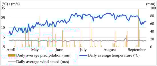
Figure 1.
Daily weather information during the observation period.
Toyota City is a coastal city located in north-central Achi Prefecture, the climate of which is characterized by hot and humid summers and is prone to marine calamity [41]. It is a city with four distinct seasons, and the weather condition changes significantly throughout the year. According to the weather data (from 1981 to 2010) released by the Japan Meteorology Agency (JMA), the second hottest month in Toyota, September, is also the wettest month of the year. The data used in this study were collected during spring and summer time, which could help in determining the impact of hot and humid weather on people’s driving habits, since the city is highly dependent on private vehicles [41].
4. Model Estimation Results
Maximum likelihood methods are used to estimate the parameter vector () in the hazard duration model. To evaluate the goodness of fit, the Akaike Information Criterion (AIC) and likelihood ratio () are used and are expressed as:
where is the number of estimable parameters in the model, is the log-likelihood of the model at convergence, and is the log-likelihood of the baseline.
To develop the model gradually, we first start with a distribution test for the daily travel distance. As mentioned above, we assume lognormal, log-logistic, and Weibull distributions. The estimated parameters are listed in Table 2, and the distribution shapes are shown in Figure 2. To clearly show the distribution shapes of the three models, Figure 2 only presents daily travel distances within 200 km, which comprise 98.62% of the whole data set. Based on the log-likelihood and the graph of distributions, the log-logistic model clearly fits the observed daily travel distance the best. The shape of the lognormal model is similar to that of the log-logistic model. The peak of the lognormal model is beyond the observed peak, and the peak of the Weibull model is a little bit short compared to the observed peak. The 95% quantile of daily travel distance for each distribution is 90 km for Weibull, 103 km for log-logistic, and 129 km for lognormal. Thus, we can assume that electric vehicles with a driving range larger than 103 km could fulfill the driving demand of our participants, and [43] mentioned 57 types of EV; only 3 of them cannot reach the need of our study. However, clearly people still have different preferences regarding the driving distance, and some people may be more adaptable to EVs, considering the battery range.
Table 2.
Estimated parameters for the three distribution models.
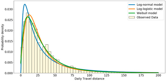
Figure 2.
Probability density for the three models.
The three distributions peak at around 10 km, and we believe that the distribution shape is affected by other covariates, such as socioeconomics. To understand how the covariates affect the daily travel distance and explain how people’s driving intention is affected by various variables, a parametric duration model is applied.
To test the heterogeneity between different individuals, the duration model was tested with pooled regression and a panel model. The results of the hazard duration models using pooled regression and the panel model are summarized in Table 3 and Table 4, respectively.
Table 3.
Model estimation results for pooled regression.
Table 4.
Model estimation results for panel data.
The AIC in Table 3 shows that the log-logistic duration model provides the best fit among the three alternatives, which is consistent with the result in Table 4. Therefore, the log-logistic duration model fits the daily travel distance best among the duration model distribution assumptions. The explanatory variables for the lognormal and Weibull duration models in Table 4 are all significant at a 95% confidence level, which can be considered an improvement compared to Table 3. However, the best fitted log-logistic model has an improvement only based on the AIC and log-likelihood ratios, but has not been improved regarding the number of significant variables.
In Table 3, at a 95% confidence level, the variables in the log-logistic model are all significant, while the lognormal model has four insignificant variables and the Weibull model has five. Even though it is mentioned in Hojati et al. [14] that weather conditions including temperature, wind speed, and precipitation do not have significant effects on traffic incident durations, these variables are found to be statistically significant in Table 3 for all the alternative duration models. Both precipitation and wind speed have a negative effect on the daily travel distance. This is consistent with our assumption that, since Toyota is a coastal city, people would be prevented from driving by heavy rains and strong winds. The weekday dummy variable as another daily information is also significant for all the alternative models. The negative effect indicates that people tend to drive longer distances during the weekend. This may be due to vehicle dependency, as well as longer travel distances to leisure areas in Toyota City. Even though the fuel efficiency is insignificant for the lognormal duration model, it still achieves a 91% confidence level with a positive effect. The main reason may be an environmental consideration, since Toyota has been selected as an environmental model city by the Japanese government [44]. The negative effect caused by the engine size may be due to the same environmental consideration, and is showing consistency over three alternative distribution assumptions.
Hybrid vehicles could be an environmentally friendly transportation mode, but it is insignificant with the Weibull model. It positively affects the travel distance in the other two models. The basic personal covariates, age and gender, are significant in all the models. Age shows a consistent negative effect for all the models, and male drivers tend to drive longer distances based on all the models. Half of the job description variables are insignificant in the lognormal duration model. The result of the Weibull model shows that only two occupations affect the travel distance. Only the variable representing those who are working as company staff is significant for all the models in Table 3, with a positive effect which indicates that they tend to drive longer than average.
Table 4 summarizes that the log-logistic duration model for the panel data is the best fitted among the alternative models, but the number of significant variables is the least. At a 95% confidence level, the variables are all significant in both the lognormal and Weibull models, but the log-logistic model has five variables that are insignificant. The improvement in the number of significant variables in the lognormal and Weibull duration models implies that the individual effect should be considered. The daily average temperature is the only daily information covariate that is not significant for the log-logistic model, which is consistent with Hojati et al. [14] and different from our expectation. However, similar as summarized in Table 3, the other weather condition variables, such as the precipitation and wind speed, along with weekday dummy in Table 4, still have negative effects on the travel distance. Except for the hybrid vehicle dummy, which is insignificant in the log-logistic model, the other vehicle information variables are all significant for all the alternative models. The result is similar to that above, showing that people who pay more for their vehicle are also willing to travel longer. The larger fuel efficiency also leads to a longer travel distance; this may cause fewer emissions when the same distance is traveled and may be one of the reasons for Toyota City being selected as an environmental model city in the pursuit of a low-carbon society [44]. Differently from Table 3, even though the engine size is still significant for all the distribution assumptions, it shows a positive effect in the Weibull duration model for the panel data. The gender variable shows the same effect as the pooled model in Table 3; males would driver longer distances than females, and as age increases the travel distance decreases. Unlike in Ding et al. [29], age is still significant for all the models, and it is found to have a negative effect on the daily travel distance. This is expected, since 98.15% of our participants are working people, and young people are always more likely to be sent by older people to do the leg work, such as sending documents to clients face to face in Japanese society. The effect of occupation is totally different from the pooled model. Six occupation variables are significant in both the lognormal and Weibull models, but only half of them are significant in the log-logistic model. The job of driving school is the only variable which shows a consistent positive effect over three models.
From the results shown in Table 3 and Table 4, even though the panel models are all improved compared to the pooled model, the lognormal duration model is not much improved compared to the other alternatives. The small magnitudes of the random parameters in the lognormal duration model implies that the individual effect is too insignificant to be considered. The Weibull and log-logistic duration models for the panel data were improved compared to the pooled models according to both the AIC and the likelihood ratio. This implies individual effects do exist and should be considered in these two duration models.
The daily average precipitation and wind speed as representative elements of weather covariates presented a consistent negative effect on the daily travel distance for all the alternative distribution assumptions in both the conventional and panel models. Similar to what was mentioned in [45], car trips are affected by rain, as people are not particularly fond of driving when the weather conditions are not good. This is quite understandable, since vehicle trips unlike railways are more flexible, and travel plans might be easily changed when people found out it is rainy, especially for the leisure trips at the weekend, since there are various alternative destinations. However, the insignificance of the daily average temperature in the log-logistic panel model was unexpected. The weekday dummy suggests that people tend to drive more during the weekend. Considering that 98.15% of the participants are employed, their driving purposes on weekdays could be quite unified as commuting. However, because of the multiple purposes for trips at the weekend and since Toyota is a vehicle-dependent city, people may still use private vehicles rather than public transportation for their leisure and other non-commuting-related trips.
The covariates of vehicle information are statistically significant at the 95% confidence level for almost all the panel duration models, except for the hybrid dummy in the log-logistic model. The positive effect produced by fuel efficiency may come with economic and environmental consequences. As mentioned in [46], a green lifestyle may lead to a person’s propensity to buy an electric vehicle, and thus the people who own better fuel efficiency vehicles may be prone to buy an electric vehicle, which holds a longer battery capacity. Household income is another widely used variable in similar studies [29,32], but since the participants were very sensitive about their income, we used the price of the vehicle to measure their willingness to pay for transportation. It is deemed that, with a consistent positive effect in both the pooled and panel models with all the distribution assumptions, people who are willing to spend more on their vehicles are also the ones who travel longer. This can be explained psychologically by what has been mentioned in [47]; those people who hold less willingness to pay for transportation may prefer living in a less car-dependent area.
The covariates of personal information—specifically, age and gender—are consistent in both the pooled and panel models with all three alternative distribution assumptions. The covariate of age reveals that older people tend to drive less than young people. Thus, different from what has been suggested in [46]—that youths share a propensity for electric vehicles—in our research, the shorter daily distance demand from older drivers could be easier fulfilled by electric vehicles. The former mainly considers people’s willingness to pay for electric vehicles, but we care more about the adaptation of people’s daily travel demands. The factor of gender indicates that males tend to drive longer than females, and this is consistent with many previous studies [29,48,49]. This may be because Japanese women are often expected to contribute themselves to the family enterprise. Even though the effect of each job is determined in the models, the result is not consistent over alternative models.
5. Conclusions
Travel behavior has been studied by examining explanatory variables in several manners. It has been demonstrated that travel distance can be used in a survival analysis as travel time [28,32]. This study developed a duration model not only with pooled regression, but also with panel data. A comparison of pooled regression and panel data models indicates that individual effects exist and can be considered using a combination of a duration model and random intercept regression. The use of lognormal, log-logistic, and Weibull models also allows an exploration of the distribution assumption for a fully parametric duration model, and here the log-logistic model demonstrated the best performance.
The daily travel distance is determined by many key factors, as tested in this study. The daily travel distance of people who live in a coastal city, such as Toyota City, is highly dependent on the weather conditions, such as precipitation and wind speed, but is not really affected by temperature during the spring and summertime as expected. The engine size, fuel efficiency, and price of the vehicle affect the travel distance significantly. Dummy variables, such as weekdays and gender, are also important in determining the travel distance. Electric vehicles a with limited battery capacity could be more adaptable to older drivers who live in a rainy and windy city, such as Toyota, and who have environmental awareness.
A limitation of this study is that even though the log-logistic panel model performed best according to the AIC and log-likelihood, the temperature variable and half of the occupational variables were insignificant. To eliminate this issue, the data observation period should be expanded to include the autumn and winter. This could help to enhance the effect of weather variables. Further research should be conducted using a random slope duration model which can also consider the individual heterogeneity. In addition, previous research also compared the travel distance by different travel purposes. In this study, we simply used a weekday dummy to differentiate commuting trips with other trips. This could be improved by the collection of trip purpose data.
Author Contributions
Conceptualization, J.H., T.Y., T.M. (Tomio Miwa), T.M. (Takayuki Morikawa); methodology, J.H., T.Y.; software, J.H., T.Y.; formal analysis, J.H.; resources, T.Y., T.M. (Tomio Miwa), T.M. (Takayuki Morikawa); writing—original draft preparation, J.H.; writing—review and editing, T.Y.; visualization, J.H.; supervision, T.Y.; project administration, T.Y.; funding acquisition, T.Y., T.M. (Tomio Miwa), T.M. (Takayuki Morikawa). All authors have read and agree to the published version of the manuscript.
Funding
This study was supported by Grant-in-Aid for Scientific Research (No. 16H02367) from the Ministry of Education, Culture, Sports, Science, and Technology, Japan, the Japan Society for the Promotion of Science. The first author graciously acknowledges the China Scholarship Council (CSC) for their financial support.
Acknowledgments
This work was carried out by the joint research program of the Institute of Materials and Systems for Sustainability and Institutes of Innovation for Future Society, Nagoya University.
Conflicts of Interest
The authors declare no conflict of interest.
References
- Washington, S.P.; Karlaftis, M.G.; Mannering, F.L. Statistical and Econometric Methods for Transportation Data Analysis, 2nd ed.; Chapman & Hall/CRC: Boca Raton, FL, USA, 2011. [Google Scholar]
- Hensher, D.A.; Mannering, F.L. Hazard-based duration models and their application to transport analysis. Transp. Rev. 1994, 14, 63–82. [Google Scholar] [CrossRef]
- Bhat, C.R.; Pinjari, A.R. Duration modeling. Handb. Transp. Model. 2000, 6, 91–111. [Google Scholar]
- Bhat, C.R.; Frusti, T.; Zhao, H.; Schönfelder, S.; Axhausen, K.W. Intershopping duration: An analysis using multiweek data. Transp. Res. Part B Methodol. 2004, 38, 39–60. [Google Scholar] [CrossRef]
- Bhat, C.R. A generalized multiple durations proportional hazard model with an application to activity behavior during the evening work-to-home commute. Transp. Res. Part B Methodol. 1996, 30, 465–480. [Google Scholar] [CrossRef]
- Niemeier, D.A.; Morita, J.G. Duration of trip-making activities by men and women. Transportation 1996, 23, 353–371. [Google Scholar] [CrossRef]
- Kharoufeh, J.P.; Goulias, K.G. Nonparametric identification of daily activity durations using kernel density estimators. Transp. Res. Part B Methodol. 2002, 36, 59–82. [Google Scholar] [CrossRef]
- Martchouk, M.; Mannering, F.; Bullock, D. Analysis of freeway travel time variability using Bluetooth detection. J. Transp. Eng. 2011, 137, 697–704. [Google Scholar] [CrossRef]
- Anastasopoulos, P.C.; Haddock, J.E.; Karlaftis, M.G.; Mannering, F.L. Analysis of urban travel times: Hazard-based approach to random parameters. Transp. Res. Rec. 2012, 2302, 121–129. [Google Scholar] [CrossRef]
- Guo, H.; Gao, Z.; Yang, X.; Zhao, X.; Wang, W. Modeling travel time under the influence of on-street parking. J. Transp. Eng. 2012, 138, 229–235. [Google Scholar] [CrossRef]
- Yu, Z.; Wood, J.S.; Gayah, V.V. Using survival models to estimate bus travel times and associated uncertainties. Transp. Res. Part C Emerg. Technol. 2017, 74, 366–382. [Google Scholar] [CrossRef]
- Bhat, C.R.; Steed, J.L. A continuous-time model of departure time choice for urban shopping trips. Transp. Res. Part B Methodol. 2012, 36, 207–224. [Google Scholar] [CrossRef]
- van den Berg, P.; Arentze, T.; Timmermans, H. A latent class accelerated hazard model of social activity duration. Transp. Res. Part A Policy Pract. 2012, 46, 12–21. [Google Scholar] [CrossRef]
- Hojati, A.T.; Ferreira, L.; Washington, S.; Charles, P. Hazard based models for freeway traffic incident duration. Accid. Anal. Prev. 2013, 52, 171–181. [Google Scholar] [CrossRef] [PubMed]
- Hasan, S.; Mesa-Arango, R.; Ukkusuri, S. A random-parameter hazard-based model to understand household evacuation timing behavior. Transp. Res. Part C Emerg. Technol. 2013, 27, 108–116. [Google Scholar] [CrossRef]
- Haque, M.M.; Washington, S. The impact of mobile phone distraction on the braking behaviour of young drivers: A hazard-based duration model. Transp. Res. part C Emerg. Technol. 2015, 50, 13–27. [Google Scholar] [CrossRef]
- Casals, L.C.; Martinez-Laserna, E.; García, B.A.; Nieto, N. Sustainability analysis of the electric vehicle use in Europe for CO2 emissions reduction. J. Clean. Prod. 2016, 127, 425–437. [Google Scholar] [CrossRef]
- Meinrenken, C.J.; Shou, Z.; Di, X. Using GPS-data to determine optimum electric vehicle ranges: A Michigan case study. Transp. Res. Part D Transp. Environ. 2020, 78, 102203. [Google Scholar] [CrossRef]
- Kempton, W.; Tomić, J. Vehicle-to-grid power fundamentals: Calculating capacity and net revenue. J. Power Sources 2005, 144, 268–279. [Google Scholar] [CrossRef]
- Guille, C.; Gross, G. A conceptual framework for the vehicle-to-grid (V2G) implementation. Energy Policy 2009, 37, 4379–4390. [Google Scholar] [CrossRef]
- Niklas, U.; von Behren, S.; Chlond, B.; Vortisch, P. Electric factor—A comparison of car usage profiles of electric and conventional vehicles by a probabilistic approach. World Electr. Veh. J. 2020, 11, 36. [Google Scholar] [CrossRef]
- Greene, D.L. Estimating daily vehicle usage distributions and the implications for limited-range vehicles. Transp. Res. Part B Methodol. 1985, 19, 347–358. [Google Scholar] [CrossRef]
- Lin, Z.; Dong, J.; Liu, C.; Greene, D. Estimation of energy use by plug-in hybrid electric vehicles: Validating gamma distribution for representing random daily driving distance. Transp. Res. Rec. 2012, 2287, 37–43. [Google Scholar] [CrossRef]
- Plötz, P.; Jakobsson, N.; Sprei, F. On the distribution of individual daily driving distances. Transp. Res. Part B Methodol. 2017, 101, 213–227. [Google Scholar] [CrossRef]
- Tamor, M.A.; Gearhart, C.; Soto, C. A statistical approach to estimating acceptance of electric vehicles and electrification of personal transportation. Transp. Res. Part C Emerg. Technol. 2013, 26, 125–134. [Google Scholar] [CrossRef]
- Li, Z.; Jiang, S.; Dong, J.; Wang, S.; Ming, Z.; Li, L. Battery capacity design for electric vehicles considering the diversity of daily vehicles miles traveled. Transp. Res. Part C Emerg. Technol. 2016, 72, 272–282. [Google Scholar] [CrossRef]
- He, J.; Yamamoto, T. Characterization of daily travel distance of a university car fleet for the purpose of replacing conventional vehicles with electric vehicles. Sustainability 2020, 12, 690. [Google Scholar] [CrossRef]
- Anastasopoulos, P.C.; Fountas, G.; Sarwar, M.T.; Karlaftis, M.G.; Sadek, A.W. Transport habits of travelers using new energy type modes: A random parameters hazard-based approach of travel distance. Transp. Res. Part C Emerg. Technol. 2017, 77, 516–528. [Google Scholar] [CrossRef]
- Ding, C.; Mishra, S.; Lu, G.; Yang, J.; Liu, C. Influences of built environment characteristics and individual factors on commuting distance: A multilevel mixture hazard modeling approach. Transp. Res. Part D Transp. Environ. 2017, 51, 314–325. [Google Scholar] [CrossRef]
- Jian, S.; Rashidi, T.H.; Wijayaratna, K.P.; Dixit, V.V. A Spatial Hazard-Based analysis for modelling vehicle selection in station-based carsharing systems. Transp. Res. Part C Emerg. Technol. 2016, 72, 130–142. [Google Scholar] [CrossRef]
- Krueger, R.; Rashidi, T. What Makes you cycle this far? An analysis of mandatory bicycle tour distances. an analysis of mandatory bicycle tour distances. SSRN Electron. J. 2017. [Google Scholar] [CrossRef]
- Anastasopoulos, P.C.; Islam, M.B.; Perperidou, D.; Karlaftis, M.G. Hazard-based analysis of travel distance in urban environments: Longitudinal data approach. J. Urban Plan. Dev. 2012, 138, 53–61. [Google Scholar] [CrossRef]
- Kleinbaum, D.G.; Klein, M. Survival Analysis; Springer: New York, NY, USA, 2010; Volume 3, pp. 35–36. [Google Scholar]
- Greene, W. Interpreting estimated parameters and measuring individual heterogeneity in random coefficient models. NYU Work. Pap. 2004. Available online: https://www.stern.nyu.edu/eco/wkpapers/workingpapers04/EC-04-08.pdf (accessed on 6 August 2020).
- Biørn, E.; Lindquist, K.G.; Skjerpen, T. Heterogeneity in returns to scale: A random coefficient analysis with unbalanced panel data. J. Product. Anal. 2002, 18, 39–57. [Google Scholar] [CrossRef]
- Kato, B.S.; Hoijtink, H. Testing homogeneity in a random intercept model using asymptotic, posterior predictive and plug-in p-values. Stat. Neerl. 2004, 58, 179–196. [Google Scholar] [CrossRef]
- Schmidheiny, K.; Basel, U. Panel data: Fixed and random effects. Short Guides Microeconometrics 2011, 7, 2–7. [Google Scholar]
- Abrevaya, J.; Shen, S. Estimation of censored panel-data models with slope heterogeneity. J. Appl. Econom. 2014, 29, 523–548. [Google Scholar] [CrossRef]
- Yang, J.; Kato, H.; Ando, R.; Nishihori, Y. Analyzing household vehicle ownership in the Japanese local city: Case study in Toyota city. J. Adv. Transp. 2018, 2020, 1–11. [Google Scholar] [CrossRef]
- von Behren, S.; Minster, C.; Esch, J.; Hunecke, M.; Vortisch, P.; Chlond, B. Assessing car dependence: Development of a comprehensive survey approach based on the concept of a travel skeleton. Transp. Res. Procedia 2018, 32, 607–616. [Google Scholar] [CrossRef]
- Yang, J.; Kato, H.; Ando, R. Comparative analysis of the household car ownership between Toyota city and Nagoya city. J. East. Asia Soc. Transp. Stud. 2015, 11, 626–639. [Google Scholar]
- Zhong, M.; Hunt, J.D.; Lu, X. Studying differences of household weekday and weekend activities: A duration perspective. Transp. Res. Rec. 2008, 2054, 28–36. [Google Scholar] [CrossRef]
- Jung, H.; Silva, R.; Han, M. Scaling trends of electric vehicle performance: Driving range, fuel economy, peak power output, and temperature effect. World Electr. Veh. J. 2018, 9, 46. [Google Scholar] [CrossRef]
- Ito, H. Toyota as an environmental model city: Is its eco-policy recognized? J. Sustain. Dev. 2014, 7, 70. [Google Scholar] [CrossRef][Green Version]
- Zanni, A.M.; Ryley, T.J. The impact of extreme weather conditions on long distance travel behaviour. Transp. Res. Part A Policy Pract. 2015, 77, 305–319. [Google Scholar] [CrossRef]
- Hidrue, M.K.; Parsons, G.R.; Kempton, W.; Gardner, M.P. Willingness to pay for electric vehicles and their attributes. Resour. Energy Econ. 2011, 33, 686–705. [Google Scholar] [CrossRef]
- Motte-Baumvol, B.; Massot, M.H.; Byrd, A.M. Escaping car dependence in the outer suburbs of Paris. Urban Stud. 2010, 47, 604–619. [Google Scholar] [CrossRef]
- Manaugh, K.; Miranda-Moreno, L.F.; El-Geneidy, A.M. The effect of neighbourhood characteristics, accessibility, home–work location, and demographics on commuting distances. Transportation 2010, 37, 627–646. [Google Scholar] [CrossRef]
- Van Acker, V.; Witlox, F. Commuting trips within tours: How is commuting related to land use? Transportation 2011, 38, 465–486. [Google Scholar] [CrossRef]
© 2020 by the authors. Licensee MDPI, Basel, Switzerland. This article is an open access article distributed under the terms and conditions of the Creative Commons Attribution (CC BY) license (http://creativecommons.org/licenses/by/4.0/).