Impact of Deforestation on Land–Atmosphere Coupling Strength and Climate in Southeast Asia


Abstract
1. Introduction
2. Data and Methods
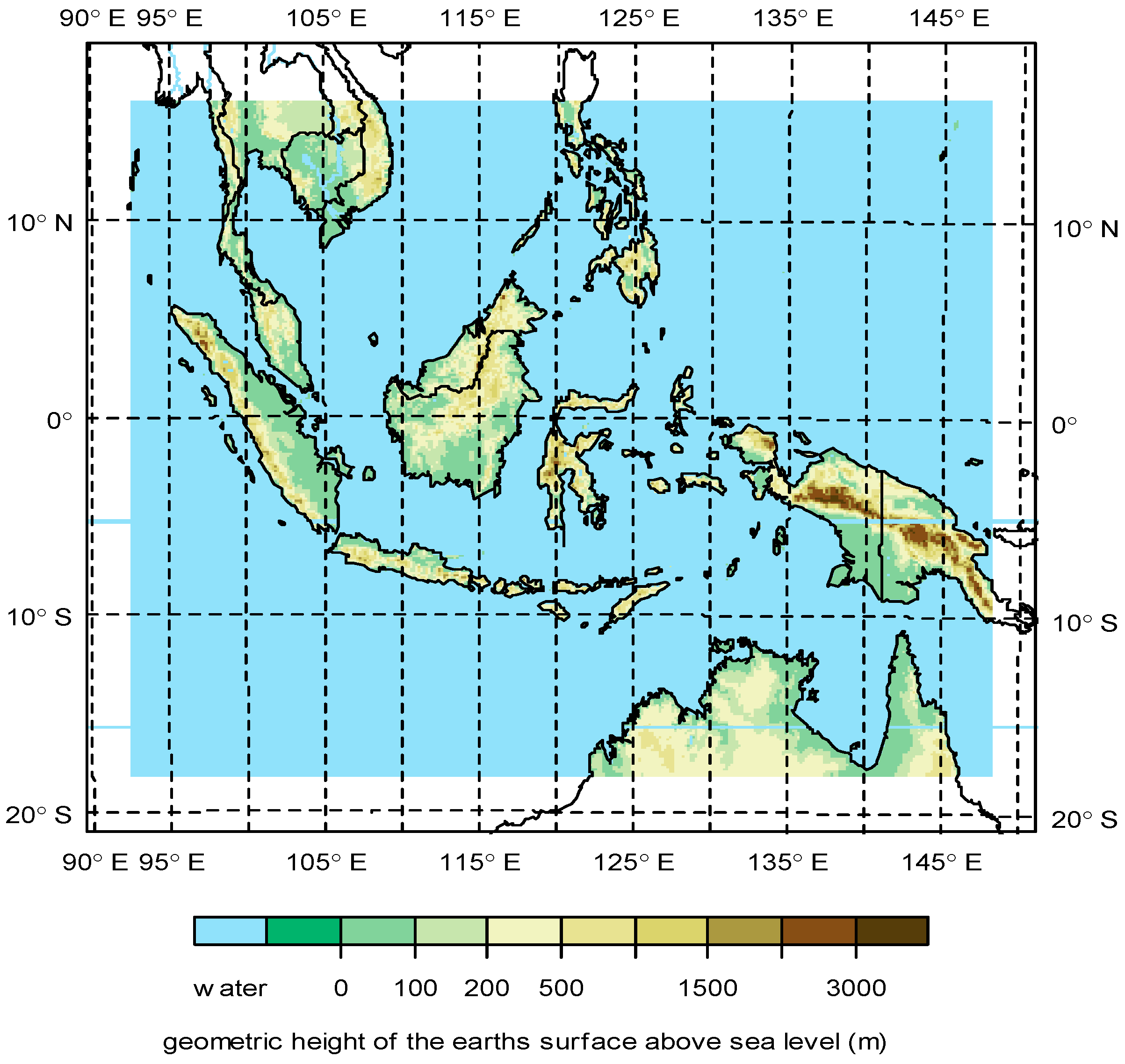
2.1. Study Region
2.2. Model Data
2.3. Coupling Concept and Analysis Method
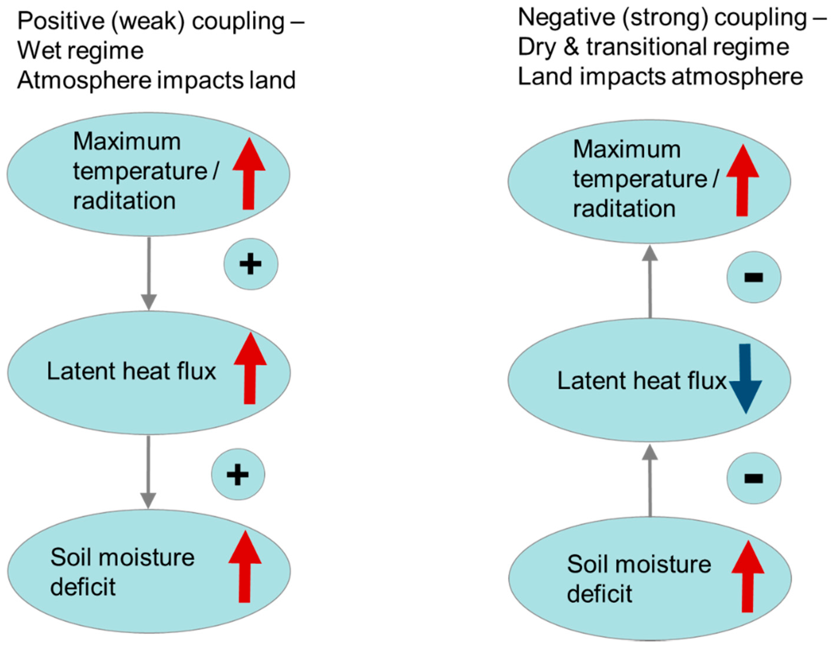
- Positive or “weak” coupling—wet regime where the atmosphere impacts the land: If sufficient soil moisture is available, the maximum air temperature dominates the near-surface atmospheric humidity and latent heat flux and with that the soil moisture. This results in positive correlations between the air temperature and latent heat flux, as well as between latent heat flux and the soil moisture deficit. Here, the atmosphere influences the land, as the soil moisture deficit is not high enough to dominate via soil moisture latent heat flux feedback.
- Negative or “strong” coupling—dry or transitional regime where land impacts the atmosphere: If sufficient soil moisture is not available, latent heat flux and also near-surface atmospheric humidity is limited by this moisture deficit, resulting in a negative correlation. If latent heat flux decreases, the maximum air temperature increases due to the lower amount of evaporative cooling, resulting in a negative correlation between the two variables. In addition, air temperature and sensible heat flux increase due to the response to increasing radiation. In this case, the land affects the atmosphere via a decrease in latent heat flux and increases in air temperature and sensible heat flux.
3. Results
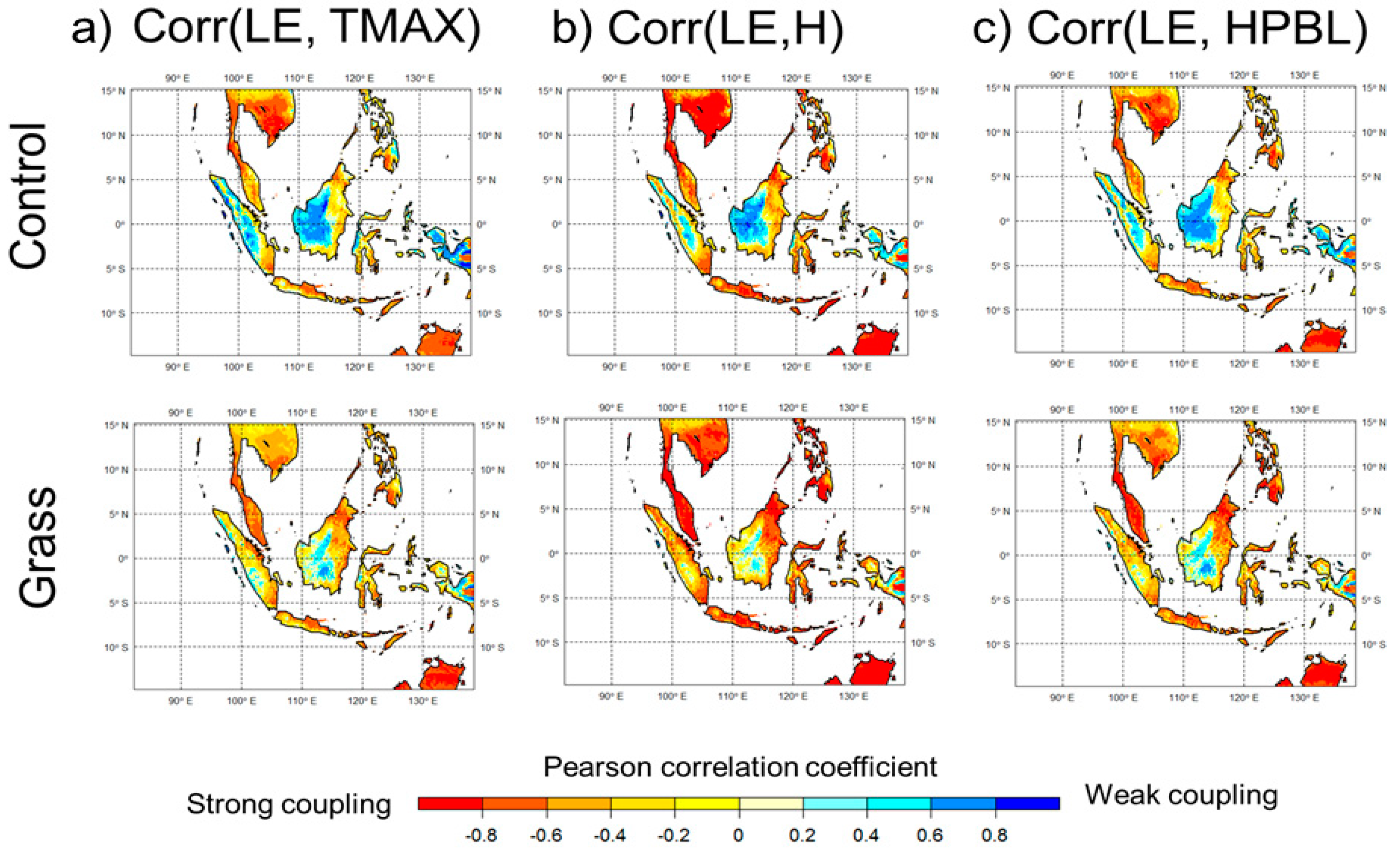
3.1. Land–Atmosphere Coupling
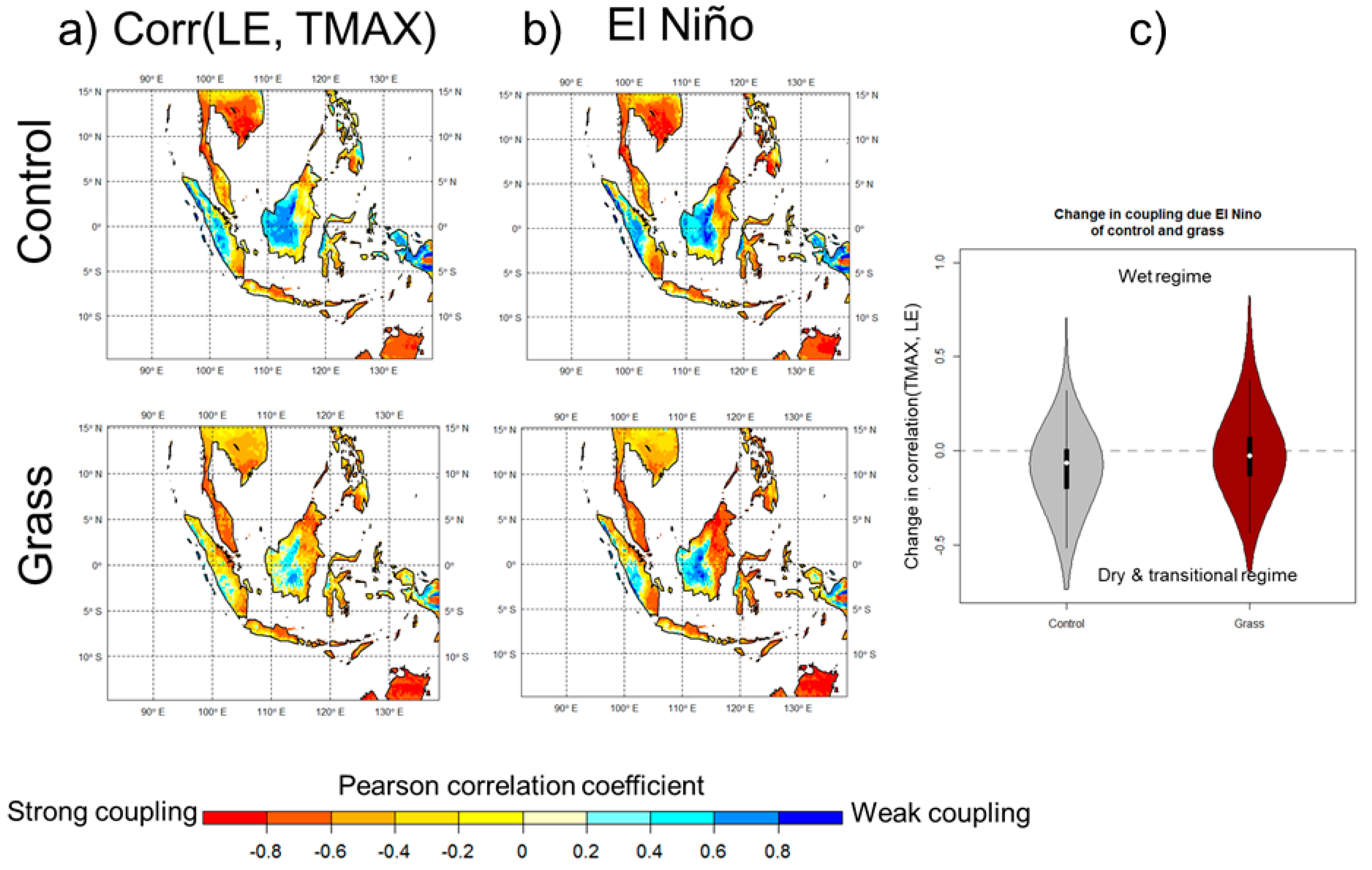
3.2. Coupling Change during El Niño
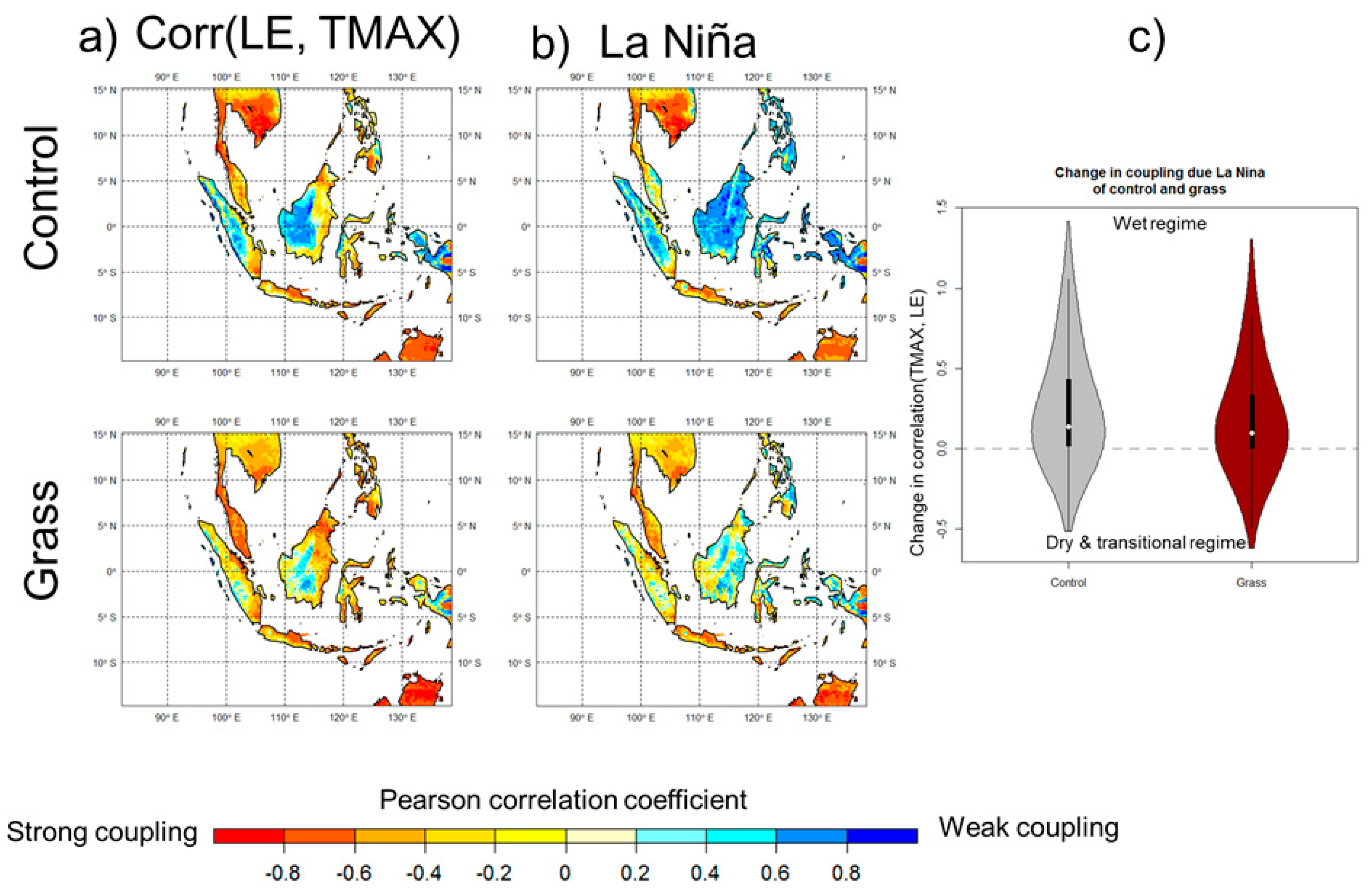
3.3. Coupling Change during La Niña
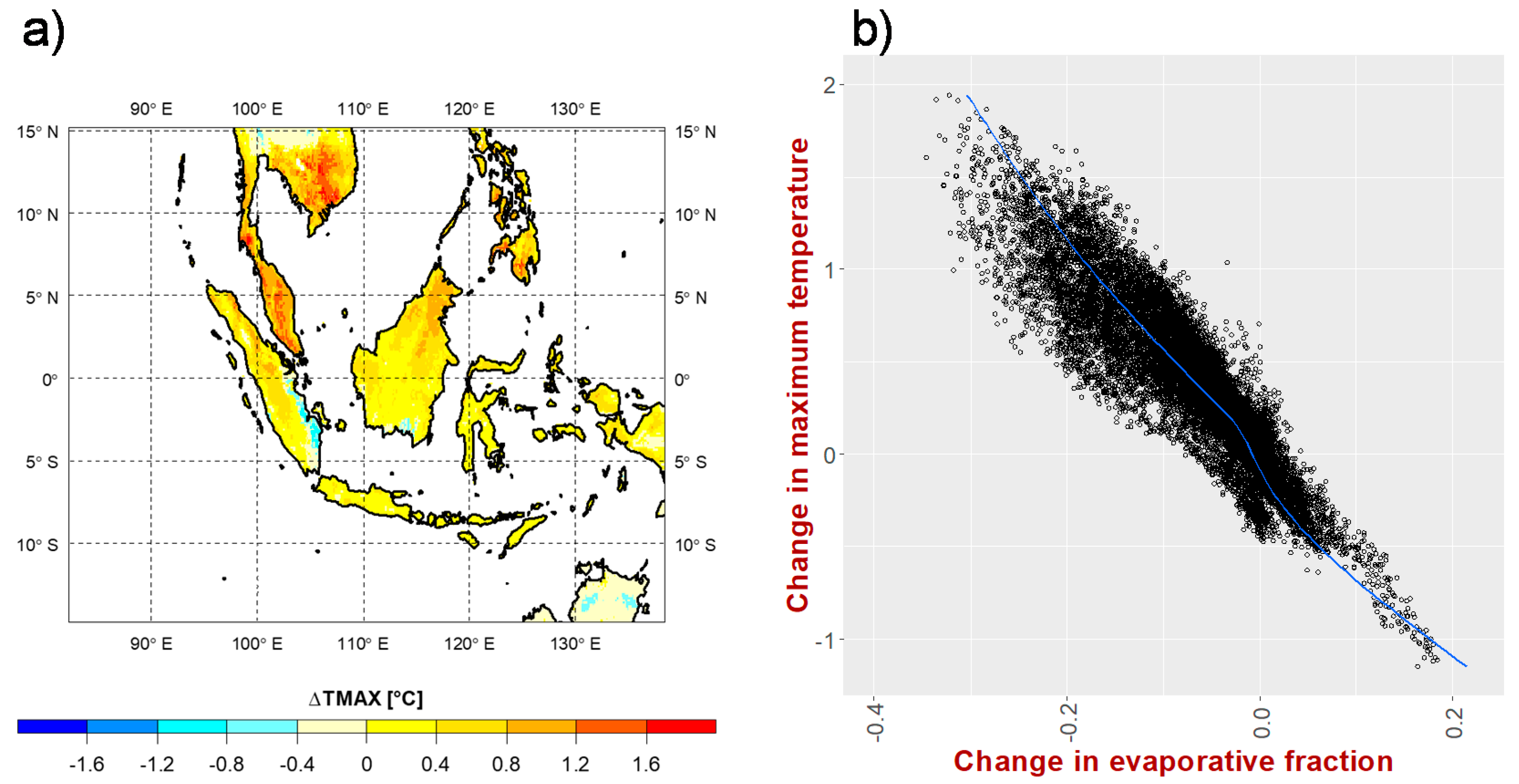
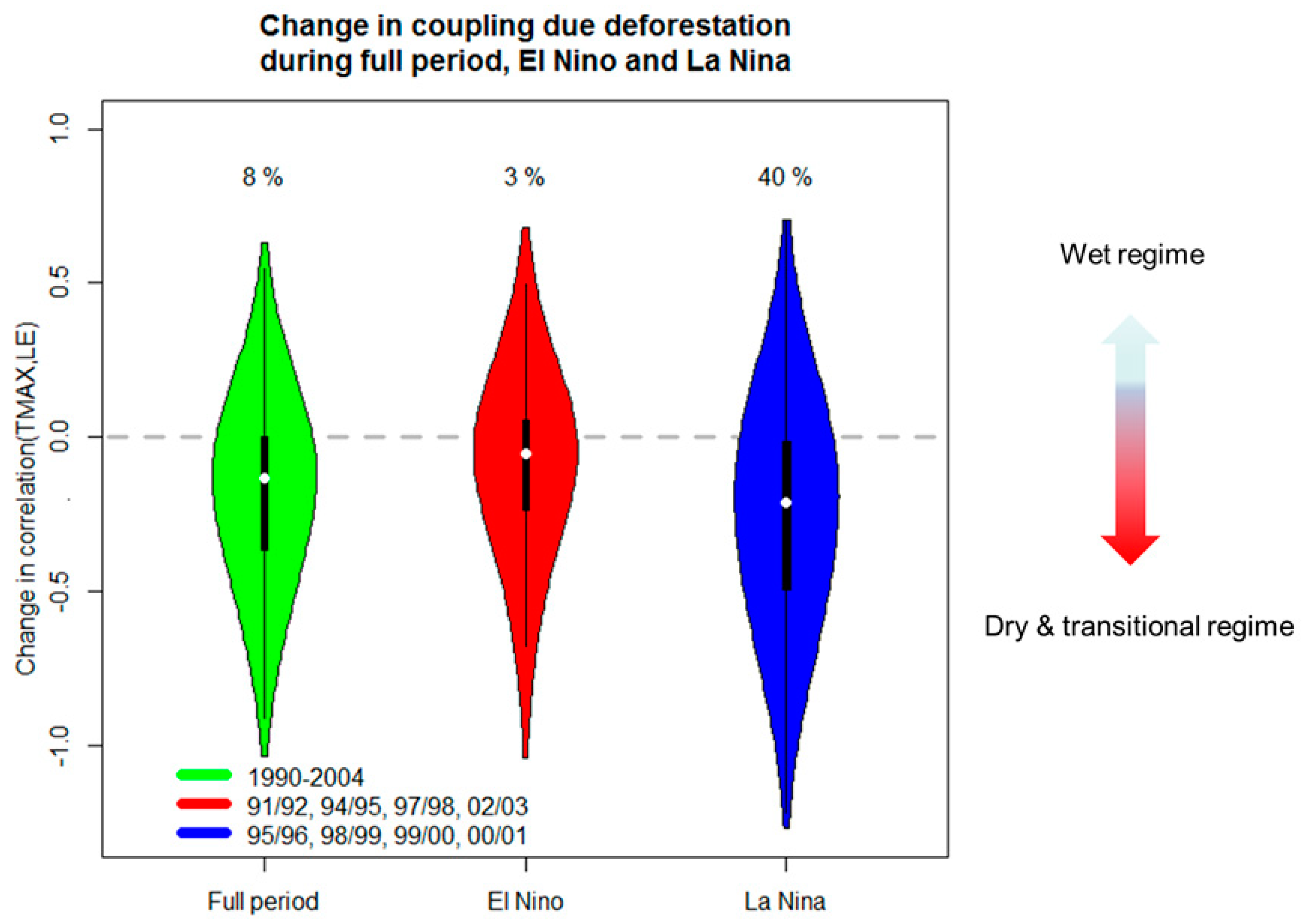
3.4. Coupling Change Due to Deforestation
4. Summary and Conclusions
Author Contributions
Funding
Acknowledgments
Conflicts of Interest
References
- IPCC. Contribution of Working Groups I, II and III to the Fifth Assessment Report of the Intergovernmental Panel on Climate Change. In Climate Change 2014: Synthesis Report; Pachauri, R.K., Meyer, L.A., Eds.; IPCC: Geneva, Switzerland, 2014; 151p. Available online: https://www.ipcc.ch/pdf/assessment-report/ar5/syr/SYR_AR5_FINAL_full_wcover.pdf (accessed on 1 May 2020).
- Stocker, T.F.; Qin, D.; Plattner, G.-K.; Alexander, L.V.; Allen, S.K.; Bindoff, N.L.; Bréon, F.-M.; Church, J.A.; Cubasch, U.; Emoir, S.; et al. Contribution of Working Group I to the Fifth Assessment Report of the Intergovernmental Panel on Climate Change. In Climate Change 2013: The Physical Science Basis; Technical Summary; Stocker, T.F., Qin, D., Plattner, G.-K., Tignor, M., Allen, S.K., Boschung, J., Nauels, A., Xia, Y., Bex, V., Midgley, P.M., Eds.; Cambridge University Press: Cambridge, UK, 2013; Available online: https://www.ipcc.ch/site/assets/uploads/2018/02/WG1AR5_TS_FINAL.pdf (accessed on 1 May 2020).
- Chape, S.; Spalding, M.; Jenkins, M.D. The World’s Protected Areas; UNEP World Conservation Monitoring Centre; University of California Press: Berkeley, CA, USA, 2008. [Google Scholar]
- Huang, C.; Goward, S.N.; Schleeweis, K.; Thomas, N.; Masek, J.; Zhu, Z. Dynamics of national forests assessed using the Landsat record: Case studies in eastern United States. Remote Sens. Environ. 2009, 113, 1430–1442. [Google Scholar] [CrossRef]
- Hansen, M.C.; Potapov, P.V.; Moore, R.; Hancher, M.; Turubanova, S.A.; Tyukavina, A.; Thau, D.; Stehman, S.V.; Goetz, S.J.; Loveland, T.R.; et al. High-resolution global maps of 21st-century forest cover change. Science 2013, 342, 850–853. [Google Scholar] [CrossRef]
- Margono, B.A.; Potapov, P.V.; Turubanova, S.; Stolle, F.; Hansen, M.C. Primary forest cover loss in Indonesia over 2000–2012. Nat. Clim. Chang. 2014, 4, 730–735. [Google Scholar] [CrossRef]
- McGrath, M.J.; Luyssaert, S.; Meyfroidt, P.; Kaplan, J.O.; Bürgi, M.; Chen, Y.; Erb, K.; Gimmi, U.; McInerney, D.; Naudts, K.; et al. Reconstructing European forest management from 1600 to 2010. Biogeosciences 2015, 12, 4291–4316. [Google Scholar] [CrossRef]
- Estoque, R.C.; Ooba, M.; Avitabile, V.; Hijioka, Y.; DasGupta, R.; Togawa, T.; Murayama, Y. The future of Southeast Asia’s forests. Nat. Commun. 2019. [Google Scholar] [CrossRef]
- Gaveau, D.L.A.; Locatelli, B.; Salim, M.A.; Yaen, H.; Pacheco, P.; Sheil, D. Rise and fall of forest loss and industrial plantations in Borneo (2000–2017). Conserv. Lett. 2018. [Google Scholar] [CrossRef]
- Oettli, P.; Behera, S.K.; Yamagata, T. Climate Based Predictability of Oil Palm Tree Yield in Malaysia. Sci. Rep. 2018, 8. [Google Scholar] [CrossRef]
- Bonan, G.B. Forests and Climate Change: Forcings, Feedbacks, and the Climate Benefits of Forests. Science 2008, 320, 1444–1449. [Google Scholar] [CrossRef]
- Pielke, R.A.; Pitman, A.J.; Niyogi, D.; Mahmood, R.; McAlpine, C.; Hossain, F.; Goldewijk, K.K.; Nair, U.S.; Betts, R.; Fall, S.; et al. Land use/land cover changes and climate: Modeling analysis and observational evidence. Clim. Chang. 2011, 2, 828–850. [Google Scholar] [CrossRef]
- Pielke, R.A.; Avissar, R.; Raupach, M.; Dolman, A.J.; Zeng, X.B.; Denning, A.S. Interactions between the atmosphere and terrestrial ecosystems: Influence on weather and climate. Glob. Chang. Biol. 1998, 4, 461–475. [Google Scholar] [CrossRef]
- Mahmood, R.; Pielke, R.A., Sr.; Hubbard, K.G.; Niyogi, D.; Dirmeyer, P.A.; McAlpine, C.; Carleton, A.M.; Hale, R.; Gameda, S.; Beltrán-Przekurat, A.; et al. Land cover changes and their biogeophysical effects on climate. Int. J. Clim. 2014, 34, 929–953. [Google Scholar] [CrossRef]
- Liu, S.; Bond-Lamberty, B.; Boysen, L.R.; Ford, J.D.; Fox, A.; Gallo, K.; Hatfield, J.; Henebry, G.M.; Huntington, T.; Liu, Z.; et al. Grand challenges in understanding the interplay of climate and land changes. Earth Interact. 2017, 21, 1–43. [Google Scholar] [CrossRef]
- Heald, C.L.; Spracklen, D.V. Land use change impacts on air quality and climate. Chem. Rev. 2015, 115, 4476–4496. [Google Scholar] [CrossRef]
- Spracklen, D.V.; Baker, J.C.A.; Garcia-Carreras, L.; Marsham, J. The Effects of Tropical Vegetation on Rainfall. Annu. Rev. Environ. Resour. 2018, 43, 193–218. [Google Scholar] [CrossRef]
- Tölle, M.H.; Gutjahr, O.; Thiele, J.; Busch, G. Increasing bioenergy production on arable land: Does the regional and local climate respond? Germany as a case study. J. Geophys. Res. Atmos. 2014, 119, 2711–2724. [Google Scholar] [CrossRef]
- Tölle, M.H.; Engler, S.; Panitz, H.-J. Impact of abrupt land cover changes by tropical deforestation on South-East Asian climate and agriculture. J. Clim. 2017, 30, 2587–2600. [Google Scholar] [CrossRef]
- Kovats, R.S.; Bouma, M.J.; Hajat, S.; Worrall, E.; Haines, A. El Niño and health. Lancet 2003, 362, 1481–1489. [Google Scholar] [CrossRef]
- Zhao, H.; Wang, C. Interdecadal modulation on the relationship between ENSO and typhoon activity during the late season in the western North Pacific. Clim. Dyn. 2016, 47, 315–328. [Google Scholar] [CrossRef]
- Zhan, R.; Wang, Y.; Zhao, J. Intensified Mega-ENSO Has Increased the Proportion of Intense Tropical Cyclones over the Western Northwest Pacific since the Late 1970s. Geophys. Res. Lett. 2017, 44, 11959–11966. [Google Scholar] [CrossRef]
- Mei, W.; Xie, S.-P.; Primeau, F.; MCWilliams, J.C.; Pasquero, C. Northwestern Pacific typhoon intensity controlled by changes in ocean temperatures. Sci. Adv. 2015, 1, e1500014. [Google Scholar] [CrossRef]
- Mei, W.; Xie, S.-P. Intensification of land falling typhoons over the northwest Pacific since the late 1970s. Nat. Geosci. 2016, 9, 753–759. [Google Scholar] [CrossRef]
- Meehl, G.A.; Stocker, T.F.; Collins, W.D.; Friedlingstein, P.; Gaye, A.T.; Gregory, J.M.; Kitoh, A.; Knutti, R.; Murphy, J.M.; Noda, A.; et al. Contribution of Working Group I to the Fourth Assessment Report of the Intergovernmental Panel on Climate Change. In Climate Change 2007: The Physical Science Basis; Global Climate Projections; Solomon, S., Qin, D., Manning, M., Chen, Z., Marquis, M., Averyt, K.B., Tignor, M., Miller, H.L., Eds.; Cambridge University Press: Cambridge, UK, 2007. [Google Scholar]
- Welker, C.; Faust, E. Tropical cyclone-related socio-economic losses in the western North Pacific region. Nat. Hazards Earth Syst. Sci. 2013, 13, 115–124. [Google Scholar] [CrossRef]
- Mei, W.; Xie, S.-P.; Primeau, F.; McWilliams, J.C.; Pasquero, C. Global warming hiatus contributed to the increased occurrence of intense tropical cyclones in the coastal regions along East Asia. Sci. Rep. 2018, 8, 6023. [Google Scholar] [CrossRef]
- Tölle, M.H.; Breil, M.; Radtke, K.; Panitz, H.-J. Sensitivity of European temperature to albedo parameterization in the regional climate model COSMO-CLM linked to extreme land use change. Front. Environ. Sci. 2018. [Google Scholar] [CrossRef]
- McAlpine, C.A.; Johnson, A.; Salazar, A.; Syktus, J.; Wilson, K.; Meijaard, E.; Seabrook, L.; Dargusch, P.; Nordin, H.; Sheil, D. Forest loss and Borneo’s climate. Environ. Res. Lett. 2018, 13, 044009. [Google Scholar] [CrossRef]
- Seneviratne, S.I.; Corti, T.; Davin, E.L.; Hirschi, M.; Jaeger, E.B.; Lehner, I.; Orlowsky, B.; Teuling, A.J. Investigating soil moisture–climate interactions in a changing climate: A review. Earth Sci. Rev. 2010, 99, 125–161. [Google Scholar] [CrossRef]
- Goddard, L. From science to service. Science 2016, 353, 1366–1367. [Google Scholar] [CrossRef] [PubMed]
- Sippel, S.; Zscheischler, J.; Mahecha, M.D.; Orth, R.; Reichstein, M.; Vogel, M.; Seneviratne, S.I. Refining multi-model projections of temperature extremes by evaluation against land-atmosphere coupling diagnostics. Earth Syst. Dyn. 2017, 8, 387–403. [Google Scholar] [CrossRef]
- Knist, S.; Goergen, K.; Buonomo, E.; Christensen, O.B.; Colette, A.; Cardoso, R.M.; Fealy, R.; Fernandez, J.; Garcia-Diez, M.; Jacob, D.; et al. Land-atmosphere coupling in EURO-CORDEX evaluation experiments. J. Geophys. Res. Atmos. 2017, 122, 79–103. [Google Scholar] [CrossRef]
- Margono, B.A.; Turubanova, S.; Zhuravleva, I.; Potapov, P.; Tyukavina, A.; Baccini, A.; Goetz, S.; Hansen, M.C. Mapping and monitoring deforestation and forestdegradation in Sumatra (Indonesia) using Landsat timeseries data sets from 1990 to 2010. Environ. Res. Lett. 2012, 7, 034010. [Google Scholar] [CrossRef]
- Doms, G.; Förstner, J.; Heise, E.; Herzog, H.-J.; Raschendorfer, M.; Schrodin, R.; Reinhardt, T.; Vogel, G. A Desciption of the Nonhydrostatic Regional Model LM. Part II: Physical Parametrization; Technical Report; Deutscher Wetterdienst: Offenbach, Germany, 2005; 133p. [Google Scholar]
- Rockel, B.; Will, A.; Hense, A. The regional climate model COSMO-CLM (CCLM). Meteorol. Z. 2008, 17, 347–348. [Google Scholar] [CrossRef]
- Dee, D.P.; Uppala, S.M.; Simmons, A.J.; Berrisford, P.; Poli, P.; Kobayashi, S.; Andrae, U.; Balmaseda, M.A.; Balsamo, G.; Bauer, D.P.; et al. The ERA-Interim reanalysis: Configuration and performance of the data assimilation system. Q. J. R. Meteorol. Soc. 2011, 137, 553–597. [Google Scholar] [CrossRef]
- Hendon, H.H. Indonesian rainfall variability: Impacts of ENSO and local air–sea interaction. J. Clim. 2003, 16, 1775–1790. [Google Scholar] [CrossRef]
- Teuling, A.J.; Taylor, C.M.; Meirink, J.F.; Melsen, L.A.; Miralles, D.G.; van Heerwarden, C.C.; Vautard, R.; Stegehuis, A.I.; Nabuurs, G.-J.; Vila-Guerau de Arellano, J. Observational evidence for cloud cover enhancement over western European forests. Nat. Commun. 2017. [Google Scholar] [CrossRef]
- Pielke, R.A. Influence of the spatial distribution of vegetation and soils on the prediction of cumulus convective rainfall. Rev. Geophys. 2001, 39, 151–177. [Google Scholar] [CrossRef]
- Dickinson, R.E. How the coupling of the atmosphere to ocean and land helps determine the timescales of interannual variability of climate. J. Geophys. Res. 2000, 105, 20115–20119. [Google Scholar] [CrossRef]
- Vereecken, H.; Schnepf, A.; Hopmans, J.; Javaux, M.; Or, D.; Roose, T.; VanderBorght, J.; Young, M.; Amelung, W.; Aitkenhead, M.; et al. Modeling Soil Processes: Review, Key Challenges, and New Perspectives. Vadose Zone J. 2016, 15. [Google Scholar] [CrossRef]
- Wang, G.; Eltahir, E.A. Biosphere-atmosphere interactions over West Africa, II, Multiple climate equilibria. Q. J. R. Meteorol. Soc. 2000, 126, 1261–1280. [Google Scholar] [CrossRef]


© 2020 by the author. Licensee MDPI, Basel, Switzerland. This article is an open access article distributed under the terms and conditions of the Creative Commons Attribution (CC BY) license (http://creativecommons.org/licenses/by/4.0/).
Share and Cite
Tölle, M.H. Impact of Deforestation on Land–Atmosphere Coupling Strength and Climate in Southeast Asia. Sustainability 2020, 12, 6140. https://doi.org/10.3390/su12156140
Tölle MH. Impact of Deforestation on Land–Atmosphere Coupling Strength and Climate in Southeast Asia. Sustainability. 2020; 12(15):6140. https://doi.org/10.3390/su12156140
Chicago/Turabian StyleTölle, Merja H. 2020. "Impact of Deforestation on Land–Atmosphere Coupling Strength and Climate in Southeast Asia" Sustainability 12, no. 15: 6140. https://doi.org/10.3390/su12156140
APA StyleTölle, M. H. (2020). Impact of Deforestation on Land–Atmosphere Coupling Strength and Climate in Southeast Asia. Sustainability, 12(15), 6140. https://doi.org/10.3390/su12156140