Optimal Reconfiguration of a Parallel Robot for Forward Singularities Avoidance in Rehabilitation Therapies. A Comparison via Different Optimization Methods

Abstract

This paper presents an efficient algorithm for the reconfiguration of a parallel kinematic manipulator with four degrees of freedom. The reconfiguration of the parallel manipulator is posed as a nonlinear optimization problem where the design variables correspond to the anchoring points of the limbs of the robot on the fixed platform. The penalty function minimizes the forces applied by the actuators during a specific trajectory. Some constraints are imposed to avoid forward singularities and guarantee the feasibility of the active generalized coordinates for a certain trajectory. The results are compared with different optimization approaches with the aim of avoiding getting trapped into a local minimum and undergoing forward singularities. The comparison covers evolutionary algorithms, heuristics optimizers, multistrategy algorithms, and gradient-based optimizers. The proposed methodology has been successfully tested on an actual parallel robot for different trajectories.

1. Introduction

Recently, there has been an increasingly growing interest in the concepts, methods, theoretical framework, and applications of mobile robots [1]. One of the most prominent applications is the use of parallel robot manipulators for rehabilitation therapies [2,3]. Parallel kinematic manipulators (PKMs) present several advantages regarding the open-chain ones, for instance, higher velocity, accuracy, rigidity, and load capability, and they present a high potential to deal with a wide range of tasks. An in-depth analysis of PKMs addressing different subjects can be found in the literature. They include aspects such as the workspace [4,5], kinematics [6,7], dynamics [8,9], elastostatics [10], motion/force transmissibility [11], robot control [12], optimal robot reconfiguration [13], robot calibration [14], and so on. Furthermore, there is exhaustive literature dealing with optimization approaches for parallel robot trajectory planning [15,16,17]. Nevertheless, they also exhibit certain disadvantages, such as limited workspace and forward kinematics singularities (FKS) [18,19,20].

A forward singularity entails the following set of characteristics: (a) at least one degree of freedom (DoF) becomes uncontrollable and a gain of at least one DoF is reached, (b) the manipulator cannot resist some wrenches applied to its platform, (c) they are not able to exit from such a singularity without external help, (d) a reduction in the robot’s workspace is attained, (e) the reactions in its joints tend to infinity, and (f) it is likely that the manipulator may adopt another assembly configuration. All these situations, particularly the loss of control, are unacceptable in a robot devoted to the rehabilitation of patients.

The disadvantages are especially significant in low-mobility PKMs, i.e., mechanisms with less than six DoF. This problem can be circumvented by rigorous trajectory planning of the robot end effector attached to the mobile platform. In this regard, the trajectory planning must consider the avoidance of the singularities within the workspace and the reduction of the actuation dynamics demands, which is carried out by the reconfiguration of the PKM. This entails that passive joints, mobile platforms, rigid links, and end effectors can be easily assembled into several configurations with different kinematic characteristics and dynamic behaviors [21].

This paper is intended to provide insight into knee rehabilitation from the geometrical and kinematical redesign of a reconfigurable PKM (RPKM). The trajectories of the mobile platform that the RPKM must follow are established by the requirements of the patient’s rehabilitation procedure and cannot be readily redesigned in advance for singularities avoidance [22,23,24]. The reconfiguration of the robot is posed as a nonlinear optimization problem subject to both linear and nonlinear constraints. The design variables are the position of the connection points for the four limbs on the mobile and fixed platform, while the objective function is the total active force needed to carry out a prescribed trajectory subject not only to several constraints on the value of the determinant of the forward Jacobian, but also to the maximum and minimum values permitted for the active generalized coordinates.

Once the problem has been raised, it is worthwhile mentioning that this paper goes a step further than previous works by comparing several optimization approaches in the framework of reconfigurable parallel robots. There is a wide range of optimization techniques that can be applied to solve the optimization problem of the parallel manipulators. The techniques compared cover evolutionary algorithms, heuristics optimizers, multistrategy algorithms, and gradient-based optimizers. An exhaustive explanation of such optimization approaches can be found, e.g., in [25]. A great effort has been made to properly compare those approaches due to the well-known difficulties in assessing their performance, as explained in [26]. Additionally, this work presents the advantage of using an efficient algorithm to solve the kinematics and dynamics of the robot manipulator. Moreover, powerful robot control is carried out by capturing the motion of the PKM mobile platform using stereophotogrammetry with a sampling rate of 25 photograms per second [27]. The location of the platform is determined, with an error lower than 0.5 mm, by three passive markers. Additionally, four markers located on the robot base define the location of the laboratory reference system. This control architecture uses open software, enables different control strategies, and is implemented using different sensors, such as potentiometers, machine vision cameras, and force sensors.

Eventually, the RPKM allows the avoidance of the forward singularities of the prescribed trajectories needed for the patient rehabilitation and the improvement of the dynamic performance of the robot by significantly reducing the forces required.

This paper is organized as follows. Section 2 presents the kinematic and dynamic modeling of the PKM, which is based on D’Alembert’s principle and the virtual power principle. This section also expounds the related forward singularities and the optimization procedure for obtaining the set of geometric parameters for the avoidance of forward singularities. It explains how this is carried out by minimizing the external forces required to execute a certain trajectory. Section 3 presents the application of the methodology to different case studies, while in Section 4 the conclusions are reported.

2. Methodology

2.1. Kinematic Model and Forward Singularities

This paper deals with the motion of a PKM for human body lower extremity rehabilitation therapies. The methodology is based on previous works [22,24] but goes a step further in improving the reconfiguration of the robot by solving the optimization problem by different optimization procedures with the aim of avoiding getting trapped into a local minimum. These optimization procedures comprise evolutionary algorithms, heuristics optimizers, multistrategy algorithms, and gradient-based optimizers. By avoiding local minima, a set of optimal parameters with a lower value of the penalty function will be achieved. Moreover, a comparison between the results is accomplished.

The methodology entails the design and dynamic analysis of a 3UPS/RPU PKM with 2T2R motion (i.e., four DoF with two translations and two rotations) for knee diagnosis and rehabilitation tasks (where U, P, R, and S stand for universal, prismatic, revolute, and spherical joints, respectively, and where the underlined letter is the actuated joint).

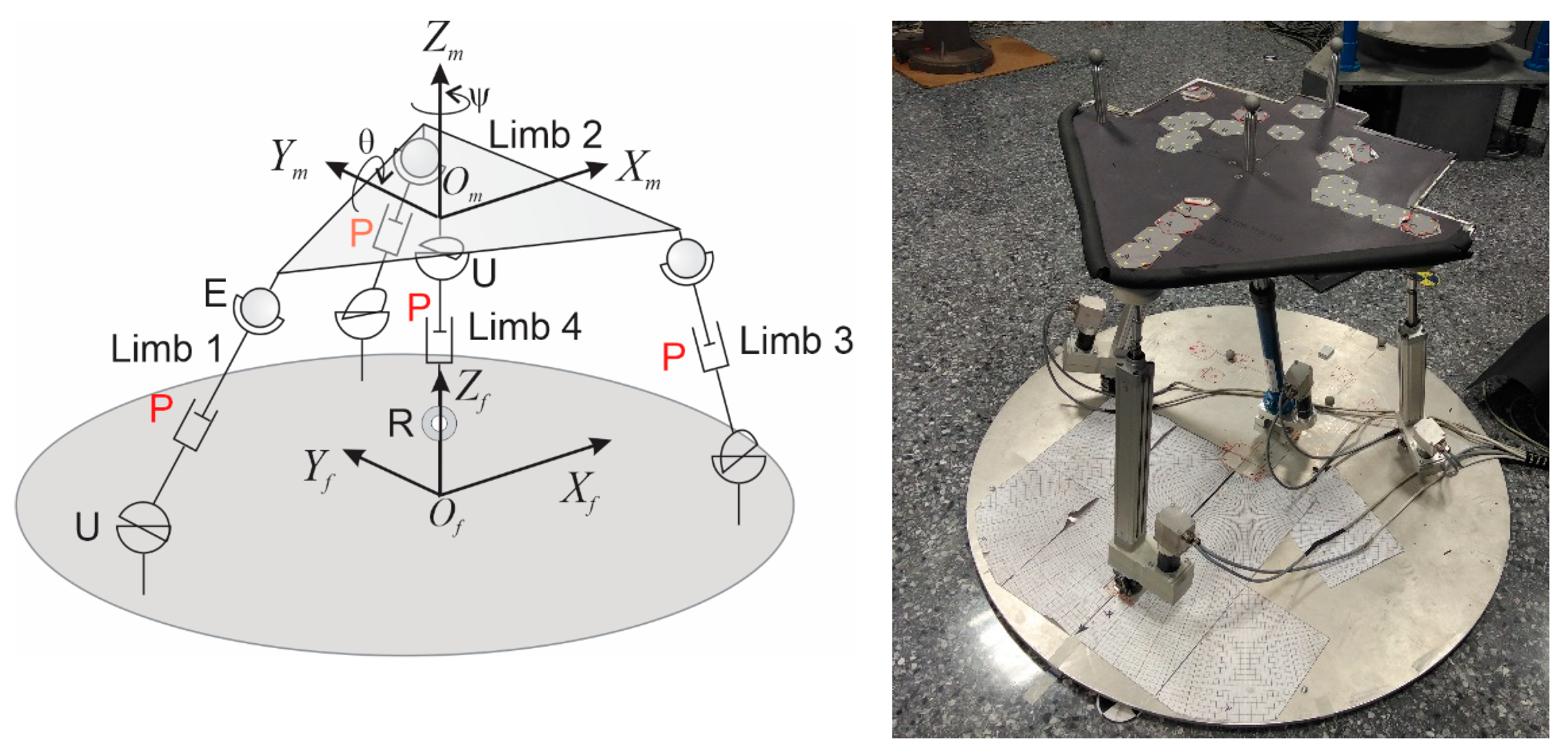
The methodology is implemented in an actual PKM with three identical external limbs comprised of universal, prismatic (actuated joints), and universal joints. Additionally, the PKM presents a central strut with rotational, prismatic (actuated joint), and universal joints. The 3UPS-RPU PKM is shown in Figure 1.

The fixed reference system is denoted by $\left\{O_f-X_f{Y}_f{Z}_f\right\}$$\left\{O_f-X_f{Y}_f{Z}_f\right\}$ while the reference system attached to the mobile platform is given by $\left\{O_m-X_m{Y}_m{Z}_m\right\}$. For the sake of conciseness, the kinematic modeling of the parallel robot is briefly presented below, while an exhaustive explanation can be found in [24].

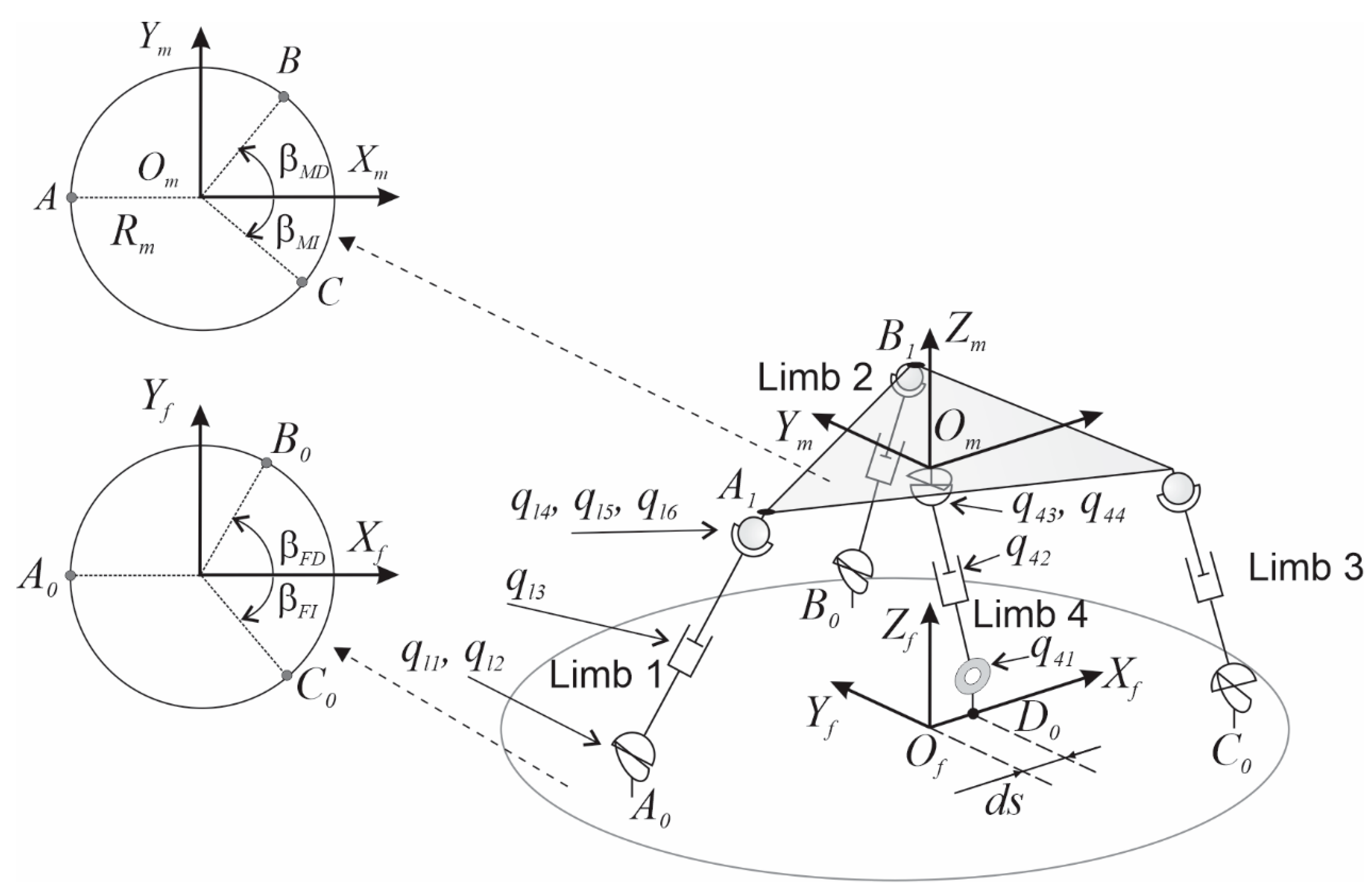
The Denavit–Hartenberg notation allows modeling the manipulator by means of a set of 22 generalized coordinates q_ij, in which the first subscript denotes the number of the limb and the second the coordinate within the limb (

Table 1. Denavit–Hartenberg parameters.

Joint	i	j	αi	ai	di	θi
Universal	1,2,3	1	−π/2	0	0	qij
	1,2,3	2	π/2	0	0	qij
Prismatic	1,2,3	3	0	0	qij	0
Spherical	1,2,3	4	π/2	0	0	qij
	1,2,3	5	π/2	0	0	qij
	1,2,3	6	π/2	0	0	qij
Revolute	4	1	−π/2	0	0	qij
Prismatic	4	2	−π/2	0	qij	π
Universal	4	3	−π/2	0	0	qij
	4	4	0	0	0	qij

).

These generalized coordinates for the external and central limbs, together with the connection points of the four limbs with both the mobile and the fixed platform, are illustrated in Figure 2.

The actuated prismatic joints represent the active generalized coordinates, i.e., q₁₃, q₂₃, q₃₃, and q₄₂. The location of the connection points is based on the radius R and the angles β_FD and β_FI for the fixed platform and R_m, β_MD, and β_MI for the mobile one. The lower connection point of the central limb (D₀) is located at a distance (ds) along the X_f axis of the fixed reference system. In addition, x_m and z_m are the coordinates of the origin of the mobile reference system. Note that y_m and φ are always zero because of the robot topology. Moreover, θand ψ represent the angles rotated by the mobile platform regarding Y_f and Z_f, respectively. Eventually, the geometric reconfiguration of the robot to be minimized is based on four geometrical parameters (R, β_FD, β_FI, and ds), which represent the design variables.

The solution of the inverse kinematic problem can be posed as a set of explicit expressions. They relate the design variables to the actuated generalized coordinates q₁₃, q₂₃, q₁₃, and q₄₂ as follows:

$$\begin{array}{c}{\mathrm{q}}_{13}=+\sqrt{\begin{array}{c}{\mathrm{R}}^2+\left(2·{\mathrm{x}}_{\mathrm{m}}-2·{\mathrm{C}}_{\mathsf{\theta }}·{\mathrm{C}}_{\mathsf{\psi }}·{\mathrm{R}}_{\mathrm{m}}\right)·R+{\mathrm{R}}_{\mathrm{m}}^2+\\ +\left(2·{\mathrm{z}}_{\mathrm{m}}·{\mathrm{S}}_{\mathsf{\theta }}-2·{\mathrm{C}}_{\mathsf{\theta }}·{\mathrm{C}}_{\mathsf{\psi }}·{\mathrm{x}}_{\mathrm{m}}\right)·{\mathrm{R}}_{\mathrm{m}}+{\mathrm{x}}_{\mathrm{m}}^2+{\mathrm{z}}_{\mathrm{m}}^2\end{array}}\\ {\mathrm{q}}_{23}=+\sqrt{\begin{array}{c}{\mathrm{R}}^2-2·\mathrm{R}·\left(\left(\begin{array}{c}{\mathrm{C}}_{\mathsf{\theta }}·{\mathrm{C}}_{\mathsf{\psi }}·{\mathrm{C}}_{\mathrm{FD}}·{\mathrm{C}}_{\mathrm{MD}}-{\mathrm{S}}_{\mathsf{\psi }}·{\mathrm{C}}_{\mathrm{FD}}·{\mathrm{S}}_{\mathrm{MD}}+\\ +{\mathrm{C}}_{\mathsf{\psi }}·{\mathrm{S}}_{\mathrm{FD}}·{\mathrm{S}}_{\mathrm{MD}}+{\mathrm{C}}_{\mathsf{\theta }}·{\mathrm{S}}_{\mathsf{\psi }}·{\mathrm{S}}_{\mathrm{FD}}·{\mathrm{C}}_{\mathrm{MD}}\end{array}\right)·{\mathrm{R}}_{\mathrm{m}}+{\mathrm{C}}_{\mathrm{FD}}·{\mathrm{x}}_{\mathrm{m}}\right)+\\ +{\mathrm{R}}_{\mathrm{m}}^2-2·{\mathrm{R}}_{\mathrm{m}}·\left({\mathrm{S}}_{\mathsf{\theta }}·{\mathrm{C}}_{\mathrm{MD}}·{\mathrm{z}}_{\mathrm{m}}+{\mathrm{S}}_{\mathsf{\psi }}·{\mathrm{S}}_{\mathrm{MD}}·{\mathrm{x}}_{\mathrm{m}}-{\mathrm{C}}_{\mathsf{\theta }}·{\mathrm{C}}_{\mathsf{\psi }}·{\mathrm{C}}_{\mathrm{MD}}·{\mathrm{x}}_{\mathrm{m}}\right)+\\ +{\mathrm{x}}_{\mathrm{m}}^2+{\mathrm{z}}_{\mathrm{m}}^2\end{array}}\\ {\mathrm{q}}_{33}=+\sqrt{\begin{array}{c}{\mathrm{R}}^2-2·\mathrm{R}·\left(\left(\begin{array}{c}{\mathrm{C}}_{\mathsf{\theta }}·{\mathrm{C}}_{\mathsf{\psi }}·{\mathrm{C}}_{\mathrm{FI}}·{\mathrm{C}}_{\mathrm{MI}}-{\mathrm{S}}_{\mathsf{\psi }}·{\mathrm{C}}_{\mathrm{FI}}·{\mathrm{S}}_{\mathrm{MI}}+\\ +{\mathrm{C}}_{\mathsf{\psi }}·{\mathrm{S}}_{\mathrm{FI}}·{\mathrm{S}}_{\mathrm{MI}}+{\mathrm{C}}_{\mathsf{\theta }}·{\mathrm{S}}_{\mathsf{\psi }}·{\mathrm{S}}_{\mathrm{FI}}·{\mathrm{C}}_{\mathrm{MI}}\end{array}\right)·{\mathrm{R}}_{\mathrm{m}}+{\mathrm{C}}_{\mathrm{FI}}·{\mathrm{x}}_{\mathrm{m}}\right)+\\ +{\mathrm{R}}_{\mathrm{m}}^2-2·{\mathrm{R}}_{\mathrm{m}}·\left({\mathrm{S}}_{\mathsf{\theta }}·{\mathrm{C}}_{\mathrm{MI}}·{\mathrm{z}}_{\mathrm{m}}+{\mathrm{S}}_{\mathsf{\psi }}·{\mathrm{S}}_{\mathrm{MI}}·{\mathrm{x}}_{\mathrm{m}}-{\mathrm{C}}_{\mathsf{\theta }}·{\mathrm{C}}_{\mathsf{\psi }}·{\mathrm{C}}_{\mathrm{MI}}·{\mathrm{x}}_{\mathrm{m}}\right)+\\ +{\mathrm{x}}_{\mathrm{m}}^2+{\mathrm{z}}_{\mathrm{m}}^2\end{array}}\\ {\mathrm{q}}_{42}=+\sqrt{{\mathrm{ds}}^2-2·\mathrm{ds}·{\mathrm{x}}_{\mathrm{m}}+{\mathrm{x}}_{\mathrm{m}}^2+{\mathrm{z}}_{\mathrm{m}}^2}\end{array}\}$$

(1)

where C_θ, S_θ, C_FD, S_FD, … stand for cos(θ), sin(θ), cos(β_FD), and sin(β_FD). The next step is to obtain the time derivative of Equation (1), which allows the relation, through a matrix expression, of the actuated generalized velocities to the velocities of the mobile platform:

$${\mathsf{\Phi }}_a·\left[\begin{array}{c}{\dot{q}}_{13}\\ {\dot{q}}_{23}\\ {\dot{q}}_{33}\\ {\dot{q}}_{42}\end{array}\right]={\mathsf{\Phi }}_x·\left[\begin{array}{c}{\dot{x}}_m\\ {\dot{z}}_m\\ \dot{\theta }\\ \dot{\psi }\end{array}\right]$$

(2)

where ${\mathsf{\Phi }}_a$ is the inverse Jacobian. For the case at hand, ${\mathsf{\Phi }}_a$ is equal to the identity matrix, which prevents the occurrence of inverse singularities in this PMK. Contrarily, the determinant of the forward (or direct) Jacobian (${\mathsf{\Phi }}_x$), which is a function of the mobile platform variables (i.e., x_m, z_m, θ, and ψ), could become zero. In that case, the PKM will undergo a forward singularity.

2.2. Dynamic Model

The dynamic model of the parallel manipulator can be obtained regardless of the generalized coordinates of the universal and the spherical joint connecting the four limbs to the platform. This allows considering a subset of the 15 following generalized coordinates:

$$\overrightarrow{q}={\left[\begin{array}{cc}\underbrace{q_{11},q_{12},q_{21},q_{22},q_{31},q_{32},q_{41},x_m,z_m,\theta ,\psi }& \underbrace{q_{13},q_{23},q_{33},q_{42}}\\ Secondary& Independent\end{array}\right]}^T$$

(3)

Therefore, the generalized coordinates can be divided into active (independent) and secondary coordinates. The augmented equation of motion for the PKM can be expressed as in Equation (4) by applying D’Alembert’s principle and the principle of virtual power:

$$\begin{array}{c}-{\overrightarrow{Q}}_{in}+{\mathsf{\Phi }}_q{}^T·\overrightarrow{\lambda }={\overrightarrow{Q}}_{grav}+{\overrightarrow{Q}}_{ex}+{\overrightarrow{Q}}_{fric}+{\overrightarrow{Q}}_{act}\\ {\mathsf{\Phi }}_q·\overrightarrow{\ddot{q}}=\overrightarrow{b}\end{array}$$

(4)

where ${\overrightarrow{Q}}_{grav}, {\overrightarrow{Q}}_{in}, {\overrightarrow{Q}}_{fric},{\overrightarrow{Q}}_{ex}, {\overrightarrow{Q}}_{act}$ are the gravitational generalized forces, the inertial generalized forces, the friction generalized forces, the external generalized forces applied to the mobile platform, and the active generalized forces exerted by the actuators, respectively. $\overrightarrow{\lambda }$ is the vector of Lagrange multipliers, $\overrightarrow{\ddot{q}}$ the generalized accelerations, and $\overrightarrow{b}$ the vector comprising the acceleration terms quadratic in velocities. Finally, ${\mathsf{\Phi }}_q$ is the Jacobian matrix related to the subsequent 11 constraint equations:

$$\begin{array}{c}{\mathsf{\Phi }}_1\equiv C_{11}·S_{12}·q_{13}-R-x_m+R_m·C_{\theta }·C_{\psi }=0 \hfill \\ {\mathsf{\Phi }}_2\equiv -C_{12}·q_{13}+R_m·C_{\theta }·C_{\psi }=0\hfill \\ {\mathsf{\Phi }}_3\equiv S_{11}·S_{12}·q_{13}-z_m-R_m·S_{\theta }=0\hfill \\ {\mathsf{\Phi }}_4\equiv C_{21}·S_{22}·q_{23}+R·C_{FD}-x_m-R_m·C_{MD}·C_{\theta }·C_{\psi }+R_m·S_{MD}·S_{\psi }=0\hfill \\ {\mathsf{\Phi }}_5\equiv -C_{22}·q_{23}+R·S_{FD}-R_m·C_{MD}·C_{\theta }·S_{\psi }-R_m·S_{MD}·C_{\psi }=0\hfill \\ {\mathsf{\Phi }}_6\equiv S_{21}·S_{22}·q_{23}-z_m+R_m·C_{MD}·S_{\theta }=0\hfill \\ {\mathsf{\Phi }}_7\equiv C_{31}·S_{32}·q_{33}+R·C_{FI}-x_m-R_m·C_{MI}·C_{\theta }·C_{\psi }-R_m·S_{MI}·S_{\psi }=0\hfill \\ {\mathsf{\Phi }}_8\equiv -C_{32}·q_{33}-R·S_{FI}-R_m·C_{MI}·C_{\theta }·S_{\psi }+R_m·S_{MI}·C_{\psi }=0 \hfill \\ {\mathsf{\Phi }}_9\equiv S_{31}·S_{32}·q_{33}-z_m+R_m·C_{MI}·S_{\theta }=0\hfill \\ {\mathsf{\Phi }}_{10}\equiv -S_{41}·q_{42}-x_m+ds=0\hfill \\ {\mathsf{\Phi }}_{11}\equiv C_{41}·q_{42}-z_m=0\hfill \end{array}$$

(5)

Equation (4) can be rewritten in matrix form and, after grouping the generalized accelerations and Lagrange multipliers on the left side of the equation, it can be expressed as follows:

$$\left[\begin{array}{cc}M& {\left({\mathsf{\Phi }}_q\right)}^T\\ {\mathsf{\Phi }}_q& O\end{array}\right]·\left[\begin{array}{c}\overrightarrow{\ddot{q}}\\ \overrightarrow{\lambda }\end{array}\right]=\left[\begin{array}{c}{\overrightarrow{Q}}_{cc}+{\overrightarrow{Q}}_{grav}+{\overrightarrow{Q}}_{ex}+{\overrightarrow{Q}}_{fric}+{\overrightarrow{Q}}_{act}\\ \overrightarrow{b}\end{array}\right]$$

(6)

where M is the mechanical system mass matrix, ${\overrightarrow{Q}}_{cc}$ are the generalized forces related to Coriolis and centrifugal accelerations belonging to ${\overrightarrow{Q}}_{in}$, and 0 is an 11 × 11 null matrix. From the different existing methods for eliminating the Lagrange multipliers [28], the coordinate partitioning method has been chosen. Equation (7) presents the matrix that relates the generalized velocities to the independent ones:

$$\left[\begin{array}{c}{\overrightarrow{\dot{q}}}^s\\ {\overrightarrow{\dot{q}}}^i\end{array}\right]=\left[\begin{array}{c}-{\left({\mathsf{\Phi }}_q^s\right)}^{-1}·{\mathsf{\Phi }}_q^i\\ 1\end{array}\right]·\left[{\overrightarrow{\dot{q}}}^i\right]$$

(7)

in which ${\mathsf{\Phi }}_q^i$, ${\mathsf{\Phi }}_q^s$ are the part of the Jacobian matrix ${\mathsf{\Phi }}_q$ related to the independent and dependent or secondary generalized coordinates, respectively, and 1 is a 3 × 3 identity matrix, hence:

$$R^{*}=\left[\begin{array}{c}-{\left({\mathsf{\Phi }}_q^s\right)}^{-1}·{\mathsf{\Phi }}_q^i\\ 1\end{array}\right]$$

(8)

The equation of motion can be compactly written as follows:

$$\begin{array}{c}{\left(R^{*}\right)}_{F\times N}^T·\left(M_{N\times N}·{\overrightarrow{\ddot{q}}}_{N\times 1}-{\overrightarrow{Q}}_{cc}{}_{N\times N}·{\overrightarrow{\dot{q}}}_{N\times 1}-{\overrightarrow{Q}}_{grav}{}_{N\times 1}-{\overrightarrow{Q}}_{fric}{}_{N\times 1}-{\overrightarrow{Q}}_{ex}{}_{N\times 1}\right)=\\ ={\left(R^{*}\right)}_{F\times N}^T·\left({\overrightarrow{Q}}_{ac}{}_{N\times F}·{\overrightarrow{F}}_{act}{}_{F\times 1}\right)\end{array}$$

(9)

where ${\overrightarrow{Q}}_{cc}$ is a matrix belonging to the centrifugal and Coriolis terms, while ${\overrightarrow{Q}}_{ac}$ is a matrix that represents the active external forces. It should be worthwhile mentioning that the right-side term of Equation (9) is the identity matrix.

$${\left(R^{*}\right)}_{F\times N}^T·{\overrightarrow{Q}}_{ac}{}_{N\times F}=1_{F\times F}$$

(10)

The equation of motion can be further developed by considering the friction force only in the prismatic actuators, thus only affecting the active generalized coordinates and changing the sign in the external and gravitational generalized forces terms:

$$\begin{array}{c}{\left(R^{*}\right)}_{4\times 15}^T·\left(M_{N\times N}·{\overrightarrow{\ddot{q}}}_{N\times 1}+{\overrightarrow{Q}}_{cc}{}_{N\times N}·{\overrightarrow{\dot{q}}}_{N\times 1}+{\overrightarrow{Q}}_{grav}{}_{N\times 1}+{\overrightarrow{Q}}_{ent}{}_{N\times 1}\right)+{\overrightarrow{F}}_{fric}{}_{F\times 1}=\\ ={\overrightarrow{F}}_{act}{}_{F\times 1}\end{array}$$

(11)

in which the friction force assigned to the generalized active coordinates is represented as:

$${\overrightarrow{F}}_{fric}=\left[\begin{array}{c}-sign\left({\dot{q}}_{13}\right)·\left({\mu }_c+{\mu }_v·\left|{\dot{q}}_{13}\right|\right)\\ -sign\left({\dot{q}}_{23}\right)·\left({\mu }_c+{\mu }_v·\left|{\dot{q}}_{23}\right|\right)\\ -sign\left({\dot{q}}_{33}\right)·\left({\mu }_c+{\mu }_v·\left|{\dot{q}}_{33}\right|\right)\\ -sign\left({\dot{q}}_{42}\right)·\left({\mu }_c+{\mu }_v·\left|{\dot{q}}_{42}\right|\right)\end{array}\right]$$

(12)

where µ_v and µ_c are the viscous and Coulomb coefficients, respectively. The determinants of both Jacobian matrices (${\mathsf{\Phi }}_q^s$ and ${\mathsf{\Phi }}_x$) vanish in the same manipulator configurations, and the latter has significantly smaller dimensions.

2.3. Objective Function and Optimization Constraints

The optimal set of geometric parameters provides the reconfiguration of the PKM for a given mobile platform trajectory. The aim of the reconfiguration procedure is to prevent the determinant of the forward Jacobian becoming null. It will avoid both the control problems associated with forward singularities and the disproportionately large control actions in the vicinity of the singular configurations despite the use of reasonable conditions of movement.

The robot manipulator design entails a set of four variables (Figure 2), which are the radius for the fixed platform (R), distance (ds), and angles of the parallel robot base (${\beta }_{FD},{\beta }_{FI}$). The physical bounds of those variables of the manipulator are:

$$\begin{array}{c}0.30\le R\le 0.50 m\\ -0.15\le ds\le 0.15 m\\ 0.10\le {\beta }_{FD}\le \frac{\pi }{2} rad\\ 0.10\le {\beta }_{FI}\le \frac{\pi }{2} rad\end{array}$$

(13)

The different rehabilitation trajectories are discretized into a sufficient number of via points (n). The objective function is computed at these points, which meets the constraint equations. The penalty function minimizes the sum of the square of the four active generalized forces. They are related to each of the configurations considered and achieved by means of the inverse dynamics of the PKM:

$$f\left(R,ds,{\beta }_{FD},{\beta }_{FI}\right)={{\displaystyle \sum }}_{i=1}^n{{\displaystyle \sum }}_{j=1}^4{F}_{ij}^2$$

(14)

where $F_{ij}$ is the generalized force on the j-th actuator for the i-th configuration of the manipulator. To ensure that the determinant ($det$) of the forward Jacobian is different from zero for all configurations considered on the trajectory, the subsequent constraints must be met:

$$\left|det\left({\mathsf{\Phi }}_{x_{ref}}\right)-det\left({\mathsf{\Phi }}_{x_i}\right)\right|<\left|det\left({\mathsf{\Phi }}_{x_{ref}}\right)\right|; i=1,2\dots ,n$$

(15)

where:

$$det\left({\mathsf{\Phi }}_{x_{ref}}\right)=max\left(det\left({\mathsf{\Phi }}_{x_i}\right)\right); i=1,2\dots ,n$$

(16)

The constraint (15) can be rewritten as in Equation (17):

$$2·det\left({\mathsf{\Phi }}_{x_{ref}}\right)·det\left({\mathsf{\Phi }}_{x_i}\right)-de{t}^2\left({\mathsf{\Phi }}_{x_i}\right)>0; i=1,2\dots ,n$$

(17)

$$\begin{array}{c}{l}_{min}\le q_{i3}\le l_{max};i=1,2,3\hfill \\ l_{min}\le q_{i2}\le l_{max};i=4\hfill \end{array}$$

(18)

with $l_{min}=0.575 m$ and $l_{max}=0.775 m$ as the minimum and maximum length of actuated joints.

$$0\le {\alpha }_i\le 0.7854 rad;i=1,2,3$$

(19)

Constraint (19) refers to the angular limits of each actuator axis with regard to the plane of the fixed platform.

The minimization of the penalty function (14) subjected to constraints (17), (18), and (19) represents a nonlinear optimization problem with nonlinear constraints that is solved by several approaches, which cover evolutionary algorithms, heuristics optimizers, multistrategy algorithms, and gradient-based optimizers.

2.4. Optimization Approaches Comparison

Optimization techniques can be classified as either local (commonly gradient based) or global (commonly nongradient based or evolutionary) algorithms. This paper compares the results among different optimization procedures, which cover evolutionary algorithms, heuristics optimizers, multistrategy algorithms, and gradient-based optimizers. However, it is worthwhile mentioning the difficulties in comparing the performance of several optimization algorithms [26]. Therefore, we have carried out the optimization algorithm comparison following the recommendations of those authors.

For the sake of conscience, only a brief description of such optimization approaches is presented, although an exhaustive explanation can be found, for instance, in [25].

(a) Evolutionary algorithm (EA) is a general term that encompasses population-based stochastic direct search algorithms, using mechanisms inspired by biological evolution, such as reproduction, mutation, recombination, and selection. They do not require any gradient information and usually make use of a set of design points (known as a population) to find the optimum design. They have the disadvantages of high computational cost, inadequate constraint-handling capabilities, specific parameter tuning for each problem, and limited problem size, and they may lead to a premature convergence to a local extremum. EA begin by generating an initial population of individuals randomly. Candidate solutions of the optimization problem emulate the role of individuals in a population. Then, an evaluation of the fitness of each individual in that population is performed (e.g., in terms of time limit, sufficient fitness achieved, etc.). Subsequently, several regenerational steps are repeated until termination, which cover the selection of the best-fit individuals for reproduction (parents), the breed of new individuals by means of crossover and mutation operations to give birth to offspring, the assessment of the individual fitness of new individuals, and the replacement of the least-fit population with new individuals. EA are suitable for all types of problems since any assumption about the underlying fitness landscape is made. Therefore, they can be applied to complex optimization problems, such as those with high dimensionality, multimodality, strong nonlinearity, and nondifferentiability, or with the presence of noise and when dealing with time dependent functions.

Among the different types of EA algorithms, we have used the multiobjective genetic algorithm (MOGA-II), the nondominated sorting genetic algorithm (NSGA-II), the adaptive range multiobjective genetic algorithm (ARMOGA), and evolution strategies (ES).

(b) Heuristic methods are designed for solving optimization problems more rapidly in cases where classic methods are too slow or fail to find any exact solution. In this sense, they trade optimality, accuracy, completeness, or precision for speed. Optimality stands for the ability to achieve the best solution, while completeness refers to the capability to provide all possible solutions for a given problem. These methods define a heuristic function, which ranks alternatives in the search algorithms at each branching step based on the available information to determine which branch to follow. They are based in finding a similar problem that has already been resolved, and determining the technique used for its resolution as well as the solution obtained.

Eventually, they lead to an approximate solution in a reasonable period of time that is suitable enough for solving the problem at hand, although the best solution may not be reached. Therefore, a drawback of these methods is the difficulty in deciding whether the provided solution is good enough, since the theory underlying these methods is not very elaborated. They are useful in problems with incomplete or imperfect information or limited computation capacity. They can also be used in conjunction with other optimization algorithms to improve their efficiency, for instance, to generate good seed values.

This work makes use of the following heuristics optimizers: multiobjective simulated annealing (MOSA) and multiobjective particle swarm optimization (MOPSO), which is inspired by the social behavior of bird flocking.

(c) Multistrategy algorithms, as the name suggests, combine the strengths of different approaches. Several approaches are used in this study. First, the multiobjective efficient global optimization (MEGO) algorithm, which is a surrogate-assisted multiobjective optimizer based on Gaussian processes. It finds the global optimum based on the fulfillment of an infill criterion for selecting search designs. MEGO is a steady-state algorithm, so it always saturates the available threads. It uses a constraint handling technique based on the probability for the design to be feasible.

Second, the FAST optimizer, which uses response surface models (RSM) (meta-models) to speed up the optimization procedure. Third, the HYBRID algorithm, which combines the global exploration abilities of genetic algorithms with the accurate local exploitation ensured by sequential quadratic programming (SQP) implementations.

Fourth, the pilOPT algorithm, which is a multistrategy self-adapting algorithm that combines the advantages of local and global search algorithms. In the search for the Pareto front, it adjusts the ratio of real and RSM-based (virtual) design evaluations based on their performance, where RSM stands for response surface methodology. It provides a remarkable performance even when handling complex output functions and constrained problems. It is generally recommended for multiobjective problems, but it can also handle single-objective problems. It is designed to work with continuous variables, but it also handles discrete variables. It does not handle categorical variables. In addition, the only parameter you need to set is the number of design evaluations, i.e., the algorithm stops when this number is reached.

(d) Gradient-based optimizers are iterative methods where the search directions are defined using the gradient information of the objective function during iterations. They provide information about the behavior of a function (shape of the surface), such as steepness and extrema in the parameter space, which may lead to drastically reduced convergence of the search algorithm. Nevertheless, this information is often not available. Specifically, we have used the Mixed Integer Programming Sequential Quadratic Programming (MIPSQP), which is based on sequential quadratic programming (SQP) and allows solving mixed integer optimization problems. SQP is an iterative method for constrained nonlinear optimization where the objective function and the constraints are twice continuously differentiable. We have also used the Levenberg–Marquardt algorithm, which is well-suited to minimizing the sum of squares of generally nonlinear functions.

Table 2. Comparison of optimization algorithms.

Method	Characteristics	Advantages	Disadvantages
Evolutionary algorithms	Mechanisms inspired by biological evolution	Global search, flexibility and adaptability, robustness, applicable to complex problems	High computational cost, requires specific adjustment of parameters, premature convergence to a local minimum
Heuristics methods	Partial search procedure that provides good enough solutions	Speed, useful under incomplete or imperfect information	Low accuracy and completeness
Multistrategy algorithms	Combine strengths of different approaches	Global optimum	Those of the techniques on which they are based
Gradient-based optimizers	Iterative methods where the search directions are defined using the gradient information of the objective function	Provides information about the shape of the objective function surface	High computational cost, local minima

presents a comparison of the optimization algorithms regarding their characteristics, advantages, and disadvantages.

Finally, all these optimization approaches are compared using the modeFRONTIER framework [29]. It allows easily coupling the different optimization algorithms with the routines that solve the kinematics and dynamics of the robot, which are implemented in FORTRAN.

3. Case Studies

The knee rehabilitation procedures to be performed by the PKM entail a set of eight test trajectories. These trajectories have been established after consulting with doctors and physiotherapists specialized in the diagnosis and rehabilitation of knee injuries. The trajectories present several difficulties during their execution, such as forward singularities or actuators out of range. Therefore, all of them are nonfeasible trajectories and require a reconfiguration.

Table 3. Definition of the eight test trajectories (Tr) and the difficulties in their execution, i.e., problems with forward singularities (1) and/or actuators out of range (2).

Trajectory	Horizontal	Vertical	Inclined Straight Line	Ellipse
Constant orientation	Tr1 (1)	Tr3 (2)	Tr5 (2)	Tr7 (1) and (2)
Variable orientation	Tr2 (1)	Tr4 (1)	Tr6 (1) and (2)	Tr8 (1) and (2)
Definition of trajectories (Tr)	Definition of trajectories by means of 11 via points (I) and their equations based on the Tait–Bryan angles (yaw, pitch, and roll)
Tr1: horizontal movement with constant orientation	$$\begin{gathered} \theta =0 \\ \psi =0 \\ {x}_m=-0.2+0.04 I \\ {z}_m=0.875 \end{gathered}$$
Tr2: horizontal movement with variable pitch angle ∈ [0°, 30°]	$$\begin{gathered} \theta =0.035 I \\ \psi =0 \\ {x}_m=-0.2+0.04 I \\ {z}_m=0.875 \end{gathered}$$
Tr3: vertical movement with a constant pitch angle of 20°	$$\begin{gathered} \theta =0.035 \\ \psi =0 \\ {x}_m=0 \\ {z}_m=0.875+0.01 I \end{gathered}$$
Tr4: vertical movement with constant yaw angle of 20°	$$\begin{gathered} \theta =0 \\ \psi =0.35 \\ {x}_m=0 \\ {z}_m=0.875+0.009 I \end{gathered}$$
Tr5: yaw movement ∊ [−20°, 20°]	$$\begin{gathered} \theta =0 \\ \psi =-0.35+0.07 I \\ {x}_m=0 \\ {z}_m=0.875 \end{gathered}$$
Tr6: inclined straight line	$$\begin{gathered} \theta =0.7854 \\ \psi =0.5236 \\ {x}_m=-0.1+0.01 I \\ {z}_m=0.63+0.01 I \end{gathered}$$
Tr7: elliptical motion with a constant pitch angle of 20°	$$\begin{gathered} \theta =0.035 \\ \psi =0 \\ {x}_m=-0.2+0.04 I \\ {z}_m=0.875+0.1\sqrt{1-{\left(\frac{x_m}{0.25}\right)}^2} \end{gathered}$$
Tr8: elliptical movement with a pitch angle ∊ [0°, 11.5°] and yaw ∊ [−17°, 17]	$$\begin{gathered} \theta =0.02 I \\ \psi =-0.3+0.06 I \\ {x}_m=-0.2+0.04 I \\ {z}_m=0.875+0.1\sqrt{1-{\left(\frac{x_m}{0.2}\right)}^2} \end{gathered}$$

illustrates the main characteristics of those trajectories regarding the motion of the mobile reference system origin and the orientation of the mobile platform. The characteristics encompass cases where the height of the mobile reference system origin is kept constant, experiences a vertical displacement, or describes a line or an ellipse in the XZ plane. Other cases are those where the orientation of the mobile platform is kept constant or varies during the movement. For all cases, the modulus of the velocity vector is constant and of an order of magnitude required in the actual rehabilitation movements. In all trajectories, 11 via points have been defined. Table 3 also depicts the difficulties found during the execution of the trajectories, i.e., problems with forward singularities and/or actuators out of range.

The reconfiguration of the robot entails four design variables $\left(R,ds,{\beta }_{FD},{\beta }_{FI}\right)$, which will be optimized and compared using different optimization techniques. There are three robot manipulator parameters that are considered to remain constant during the performance of the different trajectories $(R_m,{\beta }_{MD},{\beta }_{MI}$). The initial parameters of the manipulator are defined in Equation (20). They are intended to avoid a trivial singular configuration, which would be reached when the mobile platform was horizontal.

$$\begin{array}{c}R=43 \mathrm{cm}\\ R_m=23 \mathrm{cm}\\ ds=5 \mathrm{cm}\\ {\beta }_{FD}={45}^{°}\\ {\beta }_{FI}={48}^{°}\\ {\beta }_{MD}={90}^{°}\\ {\beta }_{MI}={100}^{°}\end{array}\}$$

(20)

Therefore, the robot parameters that are considered constant during the trajectory performance ($R_m, {\beta }_{MD}, {\beta }_{MI}$), are defined as 23 cm, 90° and 100°, respectively. The physical bounds of the four optimized design variables are those presented in Equation (13).

The physical bounds of the parallel robot are defined as follows: the actuator angles must be less than 0.7854 rad and their lengths must be between 0.575 and 0.775 m. Between those upper and lower physical bounds, all discrete configurations of the robot were obtained considering steps of 1° for angular bounds and 1 cm for length limits.

After several trial and error simulations, a reasonable set of tuning parameters has been used for all optimization techniques with the aim of achieving the lower value of the objective function while meeting all constraints.

Table 4. Optimized design variables for trajectory 2.

Algorithm	${\mathit{\beta }}_{\mathit{F}\mathit{D}} (°)$	${\mathit{\beta }}_{\mathit{F}\mathit{I}} (°)$	R (cm)	ds (cm)	Objective Function (N2)	Minimum Value of Equation (17)
Evolutionary algorithms
NSGA-II	180	48	40	15	154,547.26	1.64 × 10−4
MOGA-II	174	60	42	15	149,220.00	2.22 × 10−4
ARMOGA	84	168	32	9	143,290.00	1.82 × 10−4
Evolution strategies	180	48	32	−1	129,375.02	2.18 × 10−4
Heuristics optimizers
MOSA	84	156	32	13	147,530.00	9.39 × 10−5
MOPSO	67	21	22	−15	106,449.01	3.21 × 10−4
Multistrategy algorithms
HYBRID	174	60	42	13	150,060.00	2.11 × 10−4
pilOPT	66	18	22	−15	104,010.00	1.99 × 10−4
FAST	177	173	40	15	193,527.55	1.32 × 10−4
MEGO	63	21	20	−15	110,761.44	1.55 × 10−4
Gradient-based optimizers
MIPSQP	132	138	30	15	212,920.00	3.20 × 10−5

presents the optimized values obtained for trajectory 2 using different optimization techniques. For each optimization technique, a thousand designs are evaluated. The optimized design variables avoid forward singularities while meeting all constraints. This is demonstrated by the fact that the minimum value of Equation (17) is greater than zero. Note that in such a case, the determinant of the forward Jacobian is different from zero for all configurations considered on the trajectory, thus avoiding forward singularities (Table 4). The results show that the pilOPT algorithm outperforms the rest of the optimization strategies since it leads to a lower value of the penalty function. In other words, the sum of the square of the four active generalized forces is lower.

For the sake of conciseness, results are only presented for trajectory 2, although it is worthwhile mentioning that similar results are obtained for all trajectories. Although for the problem at hand it seems that the best choice is the pilOPT algorithm for the reconfiguration of the robot, there are other algorithms, such as the MOPSO or MEGO algorithms, with a value of the penalty function similar to that obtained with the pilOPT algorithm. Therefore, it could be expected that, with better tuning of the specific parameters of each optimization algorithm or with a greater number of design evaluations, a lower value of the penalty function would be achieved. This is because results strongly depend on the tuning of the specific parameters of each optimization algorithm, e.g., the stopping conditions, population size, step sizes, or initial penalty values [26]. On the one hand, the parameters of evolutionary algorithms, such as the mutation probability, crossover probability, and population size, should be tuned to find suitable settings for the problem class at hand. In this sense, a very small mutation rate can cause a genetic drift that is nonergodic in nature. A recombination rate that is too high may induce a premature convergence of the genetic algorithm, while a mutation rate that is too high may lead to the loss of suitable solutions, unless an elitist choice is used. On the other hand, the parameters of gradient-based optimizers should also be adjusted, such as the penalty parameter that weights a measure of the infeasibility against the value of either the objective function or the Lagrangian function.

Consequently, one of the reasons why the pilOPT algorithm provides the lower penalty function is that it only requires one parameter, which is the number of design evaluations determining when the algorithm stops. Furthermore, it can run autonomously without the need for defining any parameter. In this case, it uses the information gathered from the problem analysis to drive the optimization in the right direction and stops the run when the Pareto does not improve any further. More precisely, the run finishes when the algorithm is unable to find enough dominating designs or the designs that it finds are neither dominating nor dominated. In any case, the maximum size of the run is 100,000 designs.

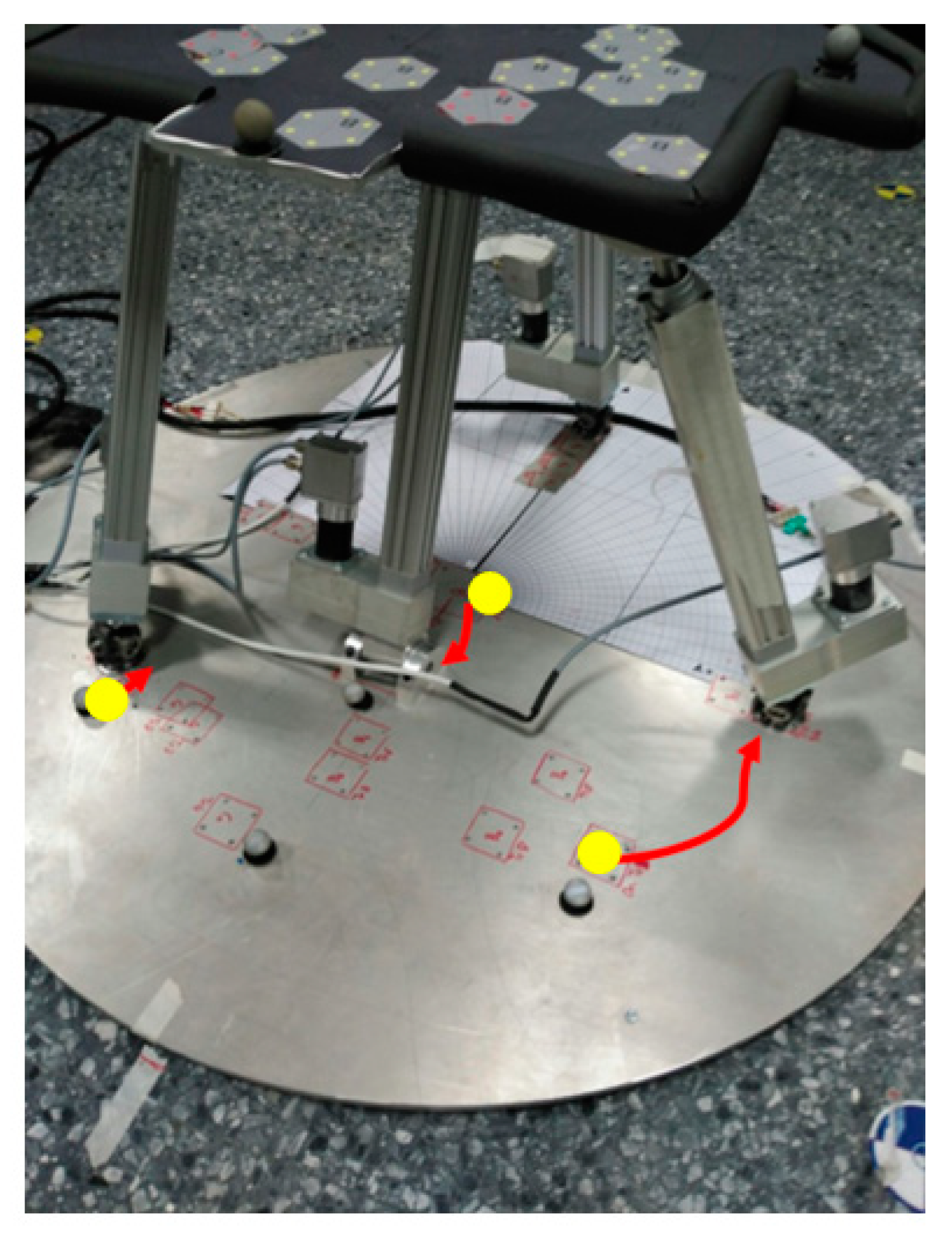
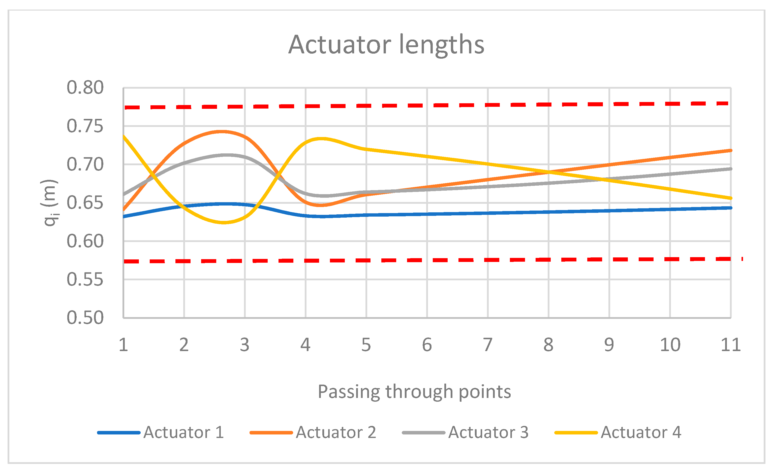
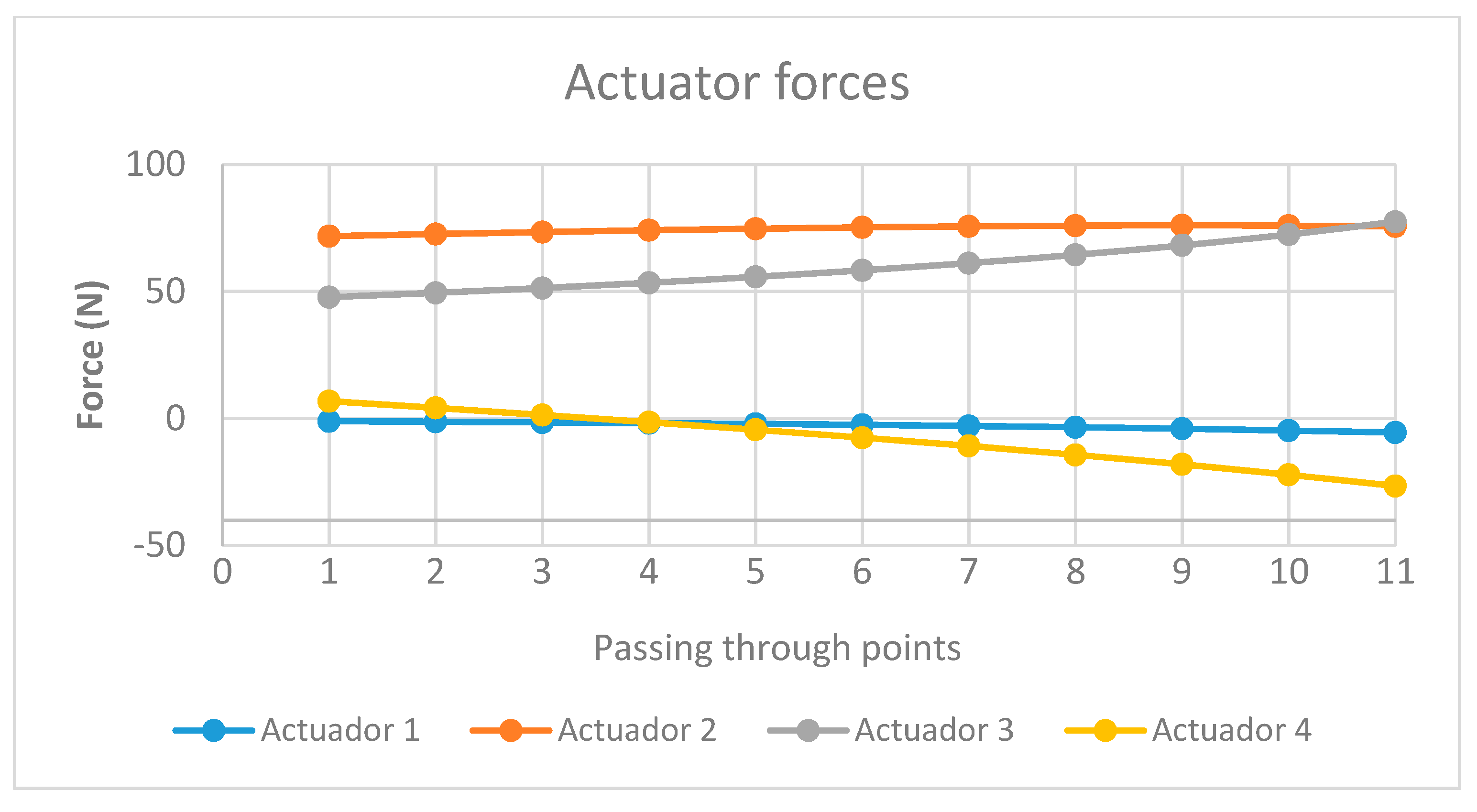
After solving the optimization problem using the pilOPT algorithm, several results are presented. Figure 3 shows the geometrical robot reconfiguration from the original robot design of the second trajectory for the fixed base.

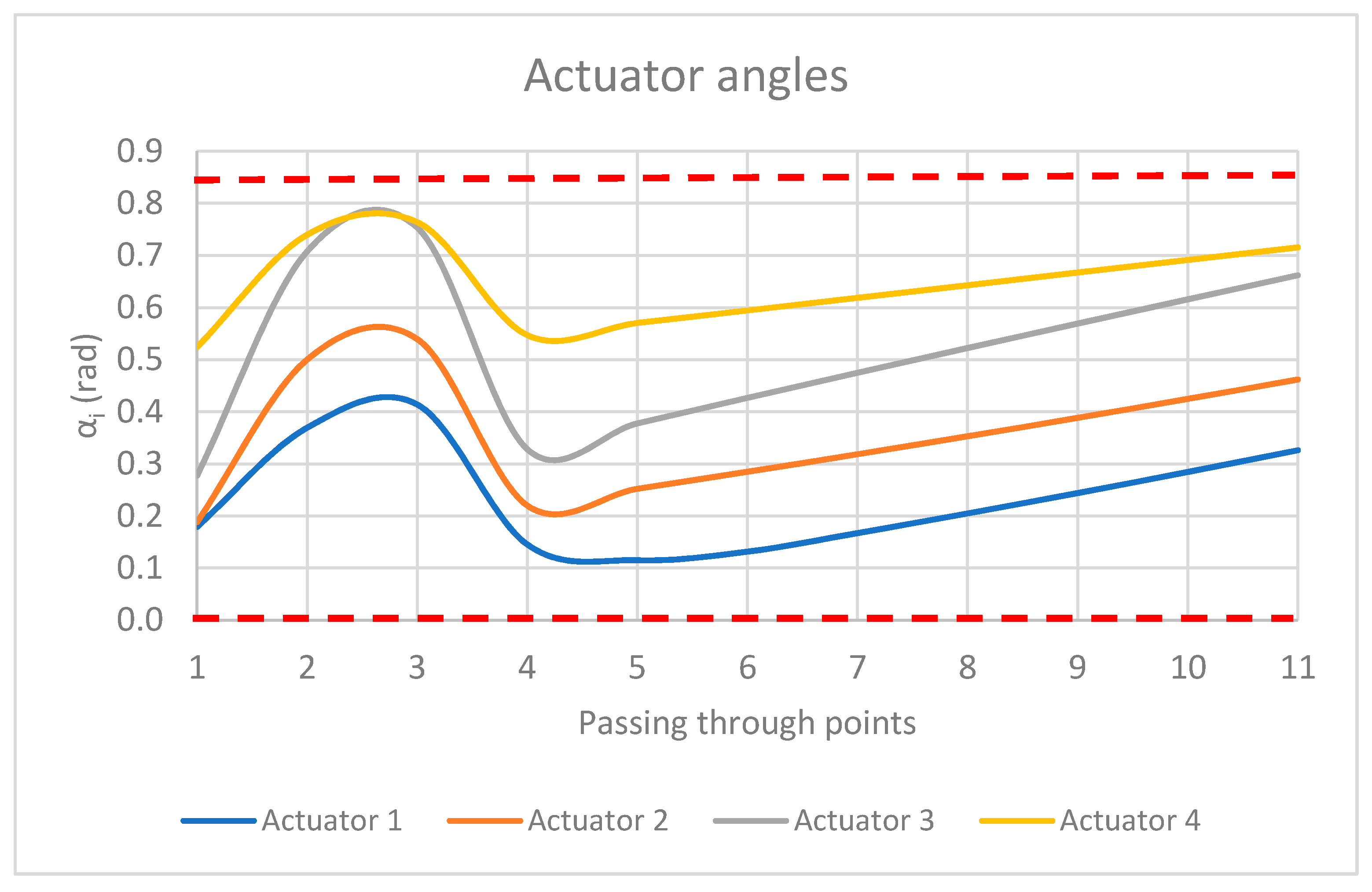
Figure 4, Figure 5 and Figure 6 depict the optimized design variables using the pilOPT algorithm and through the different robot configurations of the second trajectory: the angles, lengths, and forces for the four actuators. Throughout the trajectory, all constraints and physical bounds of the manipulator are met.

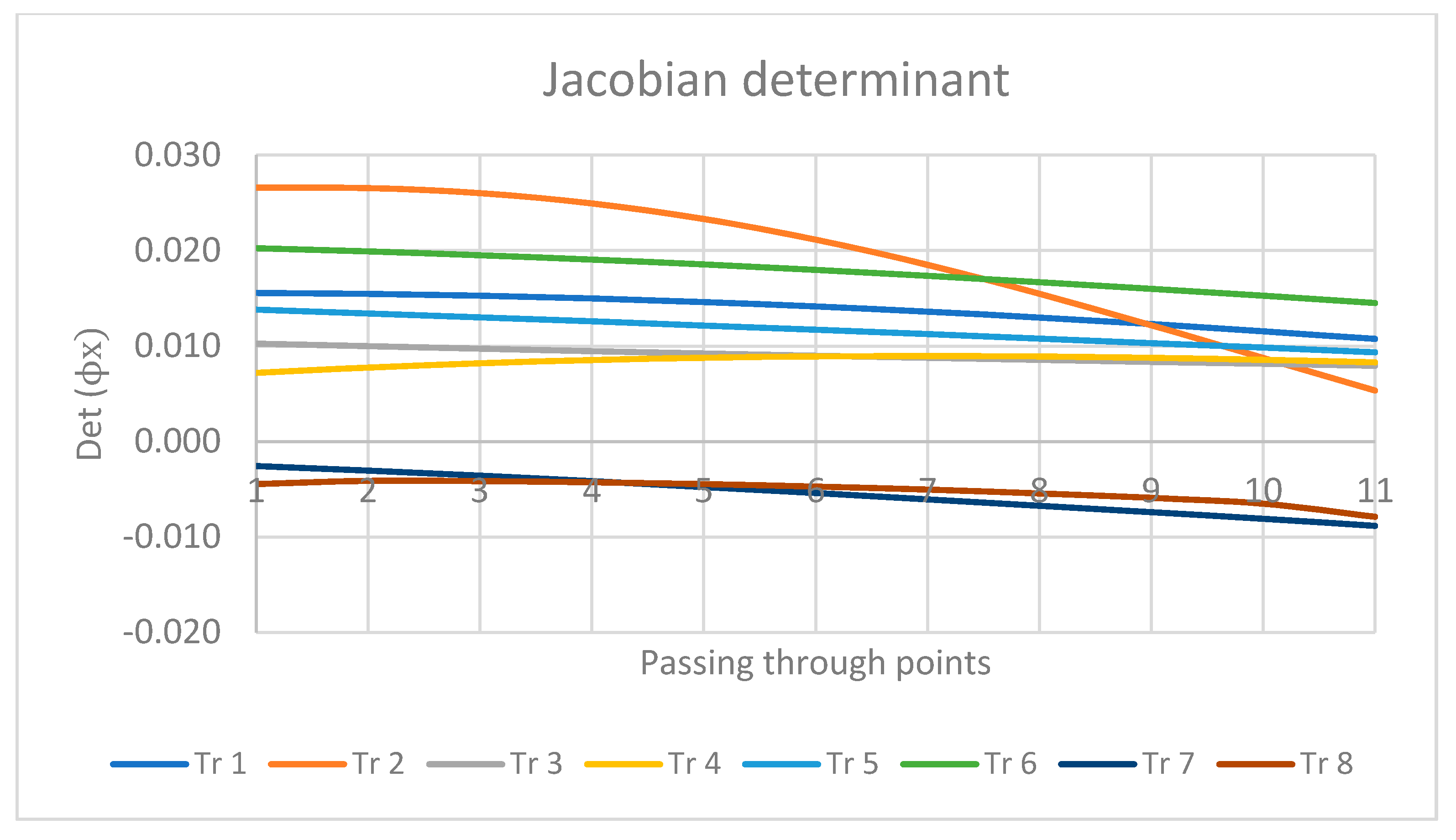
Figure 7 shows the Jacobian determinant values for the optimized design variables using the pilOPT algorithm and through the different robot configurations of all trajectories. The values are different from zero for all via points, thus avoiding forward singularities after the optimization procedure.

Bearing in mind that the pilOPT algorithm leads to the best results, the eight nonfeasible trajectories are solved using this optimization technique.

Table 5. Optimized design variables for the eight nonfeasible trajectories.

Trajectory	${\mathsf{\beta }}_{\mathbf{FD}} (°)$	${\mathsf{\beta }}_{\mathbf{FI}} (°)$	R (cm)	ds (cm)	Objective Function (N2)
1	18	30	28	−7	101,130.00
2	66	18	22	−15	104,010.00
3	60	12	30	9	79,627.00
4	60	18	36	15	58,168.00
5	72	30	26	−9	109,410.00
6	48	6	30	1	65,622.00
7	90	25	35	15	83,526.00
8	48	114	32	15	248,780.00

illustrates the optimal reconfiguration design variables of the robot using the pilOPT algorithm. The robot reconfiguration not only prevents the problem of a direct singularity, but the high values of generalized forces in its vicinity are also reduced. Moreover, the level of active forces in the rest of the via points of the trajectory is also decreased.

It has been concluded that there is not any single optimization algorithm that is the best choice for all types of optimization problems. Instead, for each problem, a certain optimization technique is more suitable, since each one has its own advantages and disadvantages. As a rule of thumb, local algorithms are more appropriate for optimization problems where the number of design variables is greater than 50, for problems with high computational cost, when numerical noise is of little significance, when gradients are easily available, and when local minima are not a problem. Contrarily, global algorithms are adequate for optimization problems where the number of design variables is less than 50, for problems with low computational cost, for combinatorial and discrete optimization problems, when numerical noise is of significance, in applications where the gradient does not exist, when there are discontinuous objective and/or constraint functions, and when a global optimum is needed. Eventually, global methods should be used only in cases where an efficient local search is not feasible.

Results show that the different optimization algorithms provide disparate results because of their specific characteristics and their pros and cons. The worth of this work is proved by the fact of the wide dispersion of the results obtained for such algorithms in both the value of the objective function and the values of the four design variables optimized, which lead to very diverse robot configurations. Therefore, when tackling optimization problems in parallel robots for rehabilitation therapies, the comparison among different optimization methods can make a difference regarding its control, safety, and dynamic behavior, which are key factors when dealing with patients.

Furthermore, this research is connected with the relatively new concept of smart health, which is influenced by several fields of knowledge, such as medical technologies, big data, artificial intelligence, communication technologies, bioengineering, robotics, machine learning, 5G and sensors, nanotechnologies, electronics, virtual and augmented reality, and so on. Furthermore, this concept is also related to the policy making and ethics that must be considered when implementing smart healthcare [30,31]. The ultimate goal is to provide patient-centered, sustainable, and efficient healthcare systems. In this sense, this work is intended to contribute to that end, since it is expected that parallel robots applied to rehabilitation therapies will be of greater use in the future because of gradual population aging, the possibility of monitoring physiological variables, the capacity of performing remote rehabilitation, the reduction in the repetitive workload of physiotherapists, and the consequent decrease in costs.

4. Conclusions

The kinematics and dynamics modeling of a PKM movement with four DoF comprised of 3UPS-RPU has been presented. It has been successfully applied to perform the required movements for diagnosis and rehabilitation tasks for human knees, specifically conditions that affect the anterior cruciate ligament. A geometrical and kinematical reconfiguration of the manipulator is posed to circumvent several problems during the execution of certain rehabilitation trajectories. These problems cover situations where the forward Jacobian becomes singular, which leads to control problems for various modes of the robot assembly and an increase in the forces required to execute the prescribed rehabilitation trajectories. Other problems encompass situations where the values needed by the active generalized coordinates lies outside the prismatic actuators’ operating ranges.

Then, the robot reconfiguration is raised as the only solution of such problems, since the rehabilitation trajectories are a priori prescribed by the physical therapists and it is not possible to modify them. The reconfiguration is carried out by modifying the points of insertion of the limbs on fixed robot platforms.

The reconfiguration problem has been posed as a nonlinear optimization problem subject to nonlinear restraints. The penalty function minimizes the sum of the square of the active generalized forces at selected via points for a certain trajectory. The constraints of the optimization problem are based on a nonsingular forward Jacobian calculated at the proposed points of the trajectory and the imposition that the active generalized coordinates fall within the admissible values of the robot actuators. The optimal redesign problem of the robot has been tackled using a dynamic inverse model of the PKM, in which D’Alembert’s principle and the principle of the virtual powers are applied. The optimization problem has been solved by means of several optimization techniques. The rehabilitation therapies cover a set of eight nonfeasible trajectories. The different optimization problems for such trajectories lead to feasible solutions while meeting all constraints. This means that, for the optimal set of parameters, the sequence of configurations does not undergo any forward singularity and the active generalized coordinates fall within the physical ranges of the actuators. Moreover, the forces required to carry out the trajectories are much lower than those of the initial configuration of the robot.

In addition, the results clearly show that the pilOPT algorithm outperforms the other algorithms for the problem at hand. This is translated for the different trajectory into higher values of the Jacobian determinant and lower lengths and forces of actuators. Furthermore, the use of a multistrategy algorithm ensures that the optimization problem has not been trapped into a local minimum.

Finally, this work demonstrates the need for performing a comparison of different optimization methods because of the wide dispersion of results that they provide, so that the comparison can make a difference regarding robot control and safety. This may prevent injuries during the rehabilitation exercises and contribute to a dynamic behavior improvement of the robot manipulator.