Abstract
Wind energy is currently one of the fastest-growing renewable energy sources in the world. For this reason, research on methods to render wind farms more energy efficient is reasonable. The optimization of wind turbine positions within wind farms makes the exploitation of wind energy more efficient and the wind farms more competitive with other energy resources. The investment costs alone for substation and electrical infrastructure for offshore wind farms run around 15–30% of the total investment costs of the project, which are considered high. Optimizing the substation location can reduce these costs, which also minimizes the overall cable length within the wind farm. In parallel, optimizing the cable routing can provide an additional benefit by finding the optimal grid network routing. In this article, the authors show the procedure on how to create an optimized wind farm already in the design phase using metaheuristic algorithms. Besides the optimization of wind turbine positions for more energy efficiency, the optimization methods of the substation location and the cable routing for the collector system to avoid cable losses are also presented.
1. Introduction
The main sources of energy are not sustainable and will be exhausted in the foreseeable future due to limited resources. In addition, conventional energy sources such as fossil fuels are leading to climate change because of global warming as a result of their large consumption by industry and society. Therefore, many researchers are in the race to find alternative energy resources, such as solar energy and wind power, to replace traditional energy sources. In particular, wind energy is considered an attractive energy source because of its advantages in terms of safety, cleanliness and above all, high yield. For this reason, the use of wind energy as a free carbon source has increased significantly in the last decades. Worldwide, the total wind power capacity has increased by , reaching 591 in 2018 from 539 in 2017.
Onshore wind parks typically cover large areas, for example, the land area required by a wind turbine can be approximately 2, so that 54 turbines would occupy around 20 2 of land area [1]. Therefore, energy companies are turning to offshore wind parks as an alternative to avoid the land rental charges that correspond to of the total operation and maintenance costs of a wind farm [1]. In addition to these advantages, offshore wind farms are more energy yielding due to the winds at sea, which could be strong over the entire day, allowing the turbine to generate more energy. However, a challenge of installing wind farms is the weight of the turbine nacelle, which typically hosts the generator, the converter, the grid-side step-up transformer as well as the monitoring and control equipment. The nacelle weight of a 5 turbine is about 300 , while the rotor is only about 120 . On average, about of the capital costs are associated with the installation in an offshore wind farm, which is as extremely high classified [1].
In general, the development and construction of a wind farm is a complex process that requires several steps to follow. The process includes the right choice of the site with the appropriate wind profile. However, wind weather data are not sufficient for the planning of a wind farm. In addition, for the economic and technical feasibility of the project, it is necessary to optimize the location of each wind turbine, optimize the location of the required substations, optimize the grid network, which connects the turbines to each other and to the substation and collects the generated energy.
Currently, several studies have investigated the wake effect generated by wind turbine blades and their impact on energy efficiency in wind farms as in [2,3]. However, the optimization of the substation location as well as the optimization of the cable layout of the power collection system has been insufficiently researched and the research lack is still large. In particular, offshore wind farms remain less explored, even though they have many advantages, which are, e.g., the favorable wind conditions that prevail on the sea due to the absence of obstacles and the low friction provided by the water. However, the construction costs for offshore wind farms remain very high and do not make them competitive with onshore wind farms. In particular, the investment costs for substation and electrical infrastructure represent 15–30% [4,5] of the total project expenditure and are classified as high. Hence, it is reasonable to optimize the wake effect for maximum energy recovery, to optimize the substation location and the electrical network in the design phase of the wind farm to shorten the investment costs for the electrical infrastructure and to decrease the cable power losses over the lifetime of the wind farm.
In this article, the authors introduce the procedure for mastering an optimal design of the wind farm layout and its optimal collector topology using metaheuristic algorithms. The paper is structured as follows. In the second part of this article, the analysis and evaluation of wind meteorological data are shown and the model for estimating the annual energy production is presented. The third section presents the optimization of wind turbine placement using a combination of the Jensen wake model and Simulated Annealing Algorithm. The fourth section focuses on the optimization of the substation location using the Particle Swarm Algorithm. In the last section of this paper, the authors show a method to optimize the grid network of a wind farm using the combination between the Genetic Algorithm and the Multiple Traveling Salesmen Problem.
2. Estimation of Annual Energy Production
2.1. Wind Data Analysis
For the calculation of the annual energy production of a wind farm and for a qualified selection of a plot or area for onshore and offshore cases, the evaluation of the wind behavior at the hub height is crucial. Mostly, meteorological measurements at the located site and at the desired altitude of over a year are taken into account [3]. However, these wind data are time series and cannot be interpreted correctly, so a probability density function of the wind speed is used for the calculation. This is usually represented by the Weibull distribution in Equation (1) [6]:
where V is the wind velocity, is the scale parameter and is the shape parameter. Figure 1 shows the two determined parameters of the Weibull distribution, which fits a histogram of discretized wind speed measurements.
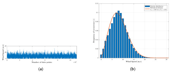
Figure 1.
Characteristics of wind data at hub height: (a) Time series of wind speed. (b) Weibull distribution.
An additional necessary characteristic is the wind direction, which indicates the installation direction of the wind turbines for a wind farm. Figure 2 shows the wind rose diagram of the wind directions. It is evident that the wind direction with the maximum frequency is on the west .
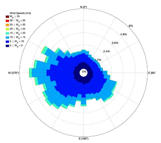
Figure 2.
Wind rose diagram.
2.2. Annual Energy Production
A wind farm consists of multiple individual wind turbines, so it is helpful to know how to calculate the annual energy production for each of them. The generated electrical power by the wind turbine is a function of wind speed and can be calculated through Equation (2) [2]:
where is the air density, A is the swept area by the blades of the wind turbine, V is the wind velocity and is the power coefficient. Figure 3 shows, for example, the power curve of the wind turbine Vestas V80-2 manufactured by the Vestas company [6]. The rated voltage of the Vestas V80-2 is 690 . The step-up transformer used inside this turbine is for a grid frequency of 50 .
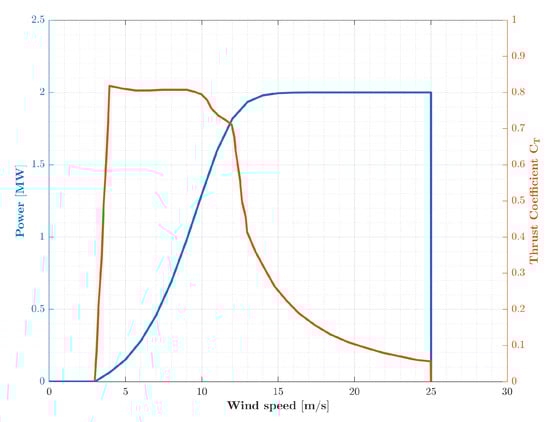
Figure 3.
Power and thrust coefficient curve of Vestas V80.
However, the weather conditions are not always the same, so the generated power depends furthermore on the frequency of occurrence of each wind speed, mentioned in Equation (1). The annual energy production can then be defined as in Equation (3):
where 8760 is the total number of hours in a year. function presents the Weibull distribution of L wind speeds and M wind directions. is the corresponding power generated by N wind turbines. The equation presents the ideal case and gives a rough estimation of annual energy production. However, it should be not forgotten that some turbines could fail and so the corresponding energy will not be produced for a while, especially in offshore wind farms, the repair can only take place in a month or more after the failure. Furthermore, the interactions between the turbines should be not neglected, represented by the wind turbulences, which strongly influence the wind speed and thus the generated power [5]. This phenomenon is called the wake effect and will be explained in detail in the following section.
3. Wind Farm Layout Optimization
3.1. Wake Model
The efficiency of a wind turbine is reduced when it is installed with other turbines in a wind farm. This is caused by changes in wind speed and the turbulence that arises behind each wind turbine due to the movement of the rotor blades. The weakening of the wind speed and thus the efficiency of a wind turbine is called the wake effect. In particular, a wind turbine behind another turbine is strongly influenced if the distance in the wind direction between the two turbines is insufficient. The wake effect in downstream wind turbines is stronger than upstream. The wind speed regains its strength after some distance behind the wind turbine. Several models can describe this effect well, such as the Larsen model [7], Frandsen model [8], Ainslie model [9] and Jensen model [10]. The Jensen Wake model is used in this article because it has proven remarkable reliability in predicting wake loss [11,12]. An illustration of the Jensen Wake model is shown in Figure 4.
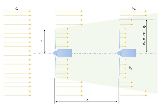
Figure 4.
Schematic of Jensen wake model between two wind turbines.
The wind velocity of the downstream wind turbine caused by an upstream wind turbine is calculated by the Equation (4) [11]:
where is the incoming wind velocity at the upstream wind turbine, is the velocity loss and can be expressed by the Equation (5) [10,11,12]:
where a is the axial induction factor, is the entrainment constant, is the downstream rotor radius and x is the downstream distance from the wind turbine that produces the wake. The entrainment constant can be determined by using the Equation (6) [11]:
where is the surface roughness length and z is the hub height of the wind turbine. The wake radius is related to the downstream distance x, the entrainment constant and the wind turbine radius r. This can be calculated by using the Equation (7) [11]:
The relationship between the thrust coefficient of the wind turbine and the axial induction factor a, which is used to calculate downstream rotor radius is given by the Equation (8) [11,12]:
Assuming that multiple wakes merge, the resulting velocity V is then calculated by equating the kinetic energy deficit of the mixed wake with the sum of the kinetic energy deficits of every wake at this point. The incoming downstream wind velocity to a wind turbine is calculated by using the Equation (10) [11,12]:
3.2. Wind Farm Efficiency
Wind farm efficiency is a useful parameter to compare the performance of the wind farm related to the power output of a single wind turbine. It can be described as in Equation (11) [2]:
where N is the number of wind turbines, is the power output of a wind turbine functioning as a single turbine and is the total power generation in the wind farm. can be obtained using the Equation (12) [13]:
where is the power generated by the i-th wind turbine in the wind farm and is given by Equation (2). For the optimization of a wind farm layout, the Equation (11) can be adopted as an objective function to maximize energy efficiency.
3.3. Cost Model
The total cost function, most used in the literature, was developed by Mosetti et al. presented in [14]. This mainly depends on the wind turbines number N as expressed in the Equation (13):
The optimization of a wind farm layout cannot only be based on energy generation, therefore the above equation is used in the optimization, representing the financial aspect for the feasibility of the project. As a result, the objective function in the Equation (14) is mostly used to optimize the wind farm layout:
Figure 5 shows that the total cost approximates linear function when N exceeds 50 wind turbines. This represents a problem in the design of a large-scale wind farm. In this case, the cost function is expressed by the Equation (15):
and thus the objective function turns into approximately by the Equation (16):
which in reality corresponds to a kind of average of the power output of each individual wind turbine. In these circumstances, maximizing the aggregate power output of the wind farm regardless of the cost function is sufficient.
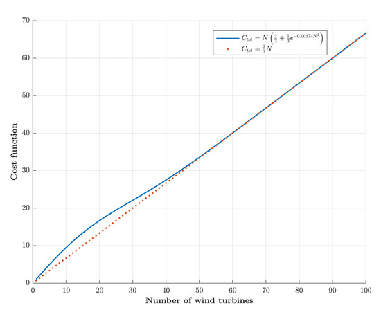
Figure 5.
Cost function of a wind farm.
Another way to optimize a wind farm layout is to minimize the following objective function in Equation (17), which is the inverse of the Equation (14):
This is mainly used to score the maximum power output of the wind farm with minimum investment costs.
3.4. Optimization with Simulated Annealing
The origin of Simulated Annealing lies in the analogy to metallurgy. It consists of raising the temperature of a solid to high values in order to reach its low energy states [15]. When the solid is at a high temperature, each particle has very high energy and can make a large set of random movements in the matter. As the temperature drops, each particle loses energy and its ability to move is reduced. Due to the different temporary cooling conditions, very homogeneous materials of good quality can be obtained.
The Simulated Annealing was developed independently by [16,17], with the basic idea that with decreasing temperature steps, the algorithm uses the iterative procedure, to reach a thermodynamic quasi-equilibrium state. This procedure makes it possible to leave the local minima with a higher probability the higher the temperature is. When the algorithm reaches very low temperatures, the most probable states are in principle excellent solutions to the optimization problem.
At the beginning of the process, the algorithm is initialized at a high temperature and then for each optimization parameter, random movements are performed. The objective function is evaluated and compared with the previous value for each of these movements. The current values of the parameters are accepted in case of gain. Otherwise, these parameters can be accepted anyway with a certain Boltzmann probability [15]:
where is the difference between the previous and current values of the objective function, T is the temperature and is the Boltzmann constant.
For the following the classical law is employed, where is the cooling coefficient. This process is repeated for a fixed number of temperature steps whereby the temperature is updated. The sequence of generated points normally converges towards the global minimum.
Normally, a sufficiently high initial temperature is chosen to allow more freedom for exploring the search space. Then, step by step, the temperature decreases until it reaches a value close to 0, which means that the method will no longer accept to worsen the solution. The flowchart in Figure 6 shows the main steps of the Simulated Annealing Algorithm.
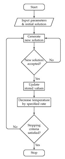
Figure 6.
Flowchart of the Simulated Annealing Algorithm.
3.5. Optimization of Wind Turbines Placement
For the optimization approach of the placement for the wind turbines, the previously mentioned objective function (17) is applied. The parameters listed in Table 1 can be used for this purpose. Additionally, it is assumed that the wind farm total area is 2 and is planar. The total area of the wind farm is divided into smaller area segments of a size of 2, where the wind turbines should be positioned in the center of the cells. Thus, the minimum distance between two adjacent wind turbines is 250 . For this approach of optimization, a unidirectional wind speed is considered.

Table 1.
Wind turbine and wind farm specifications.
From Figure 7b it can be seen that the Simulated Annealing Algorithm for this optimization problem finds a minimum of the objective function already at approximately the 350th iteration. The optimal placement of the wind turbines within the given wind farm area can be seen in Figure 7a. The improvement of the fitness value compared to the one of the initial solution for the wind turbine distribution is approximately . The minimizing of the objective function also leads to the maximizing of the power production of the wind farm.
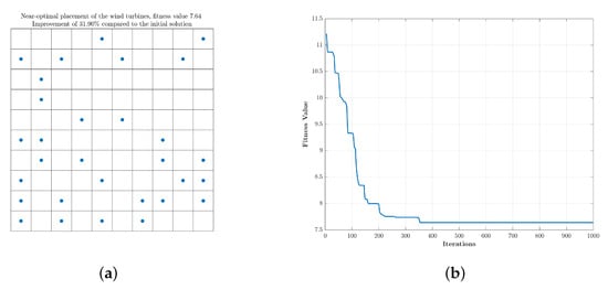
Figure 7.
Location optimization of 30 wind turbines in a 2 wind farm: (a) Locations of wind turbines. (b) Convergence curve.
Under the same conditions given in Table 1, the optimization approach using Simulated Annealing is applied to design 70 wind turbines within a wind farm with a total area of 25 2. Figure 8 shows the optimized wind turbine placements and the corresponding convergence curve. An improvement of approximately can be achieved within 300 iterations when compared to the initial solution.
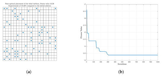
Figure 8.
Location optimization of 70 wind turbines in a 2 wind farm: (a) Locations of wind turbines. (b) Convergence curve.
4. Optimization of Substation Location
4.1. Optimization Model for Substation Location
A substation is a transformer platform, which is mainly used for offshore wind farms in the open sea. The substation is designed to reduce losses and the effort required to transmit electrical energy from the offshore wind farm to the mainland. An offshore wind farm can consist of several hundreds of individual wind turbines, which are usually divided into groups or clusters. The wind turbines of each cluster are connected to each other by submarine cables, known as feeders, that are laid in a ring or radial pattern in the wind farm to the transformer substation. Figure 9 shows the radial as well as the ring wind farm topology.
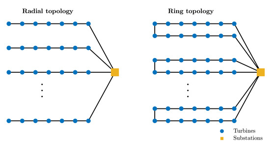
Figure 9.
Illustration of radial and ring topology.
The main task of the offshore substation is to bring together the feeders of the individual wind turbines or the clusters of a wind farm and to transform the voltage from the medium-voltage level of the wind farm system to the corresponding high-voltage system for subsequent transmission [18]. The specific space requirement of the substation is about 200 2 per 100 of power. Small wind farms with few turbines and a capacity of less than 100 or farms whose internal voltage level corresponds to the grid voltage at the point of entry, can dispense with a transformer substation if the distance to the shore is less than 15 . The substation with the transformer on the platform serves as a collection point or as a collection system. In the transformer station, the electricity generated is transformed from the voltage level within the wind farm, typically 33 , to the voltage level of the high-voltage grid, typically in the range of 100–200 . On the one hand, this reduces the electrical power losses due to the transmission on the way to the coast. On the other hand, the outgoing cables can transmit a considerably higher power due to the higher voltage, which reduces the number of cables to be laid to the mainland.
In addition to their electrical function, transformer platforms often also serve as a base for construction, maintenance and inspection work on the wind farm.
Besides all these tasks of the transformer station, which mainly reduce the electrical power losses in the transmission line to the shore, the energy efficiency can be furthermore improved through the optimization of the substation’s location within the wind farm. With the adequate placement of the substation, the power losses caused by the feeders from the wind turbines to the substation can be reduced. In addition to the above mentioned advantages, economic benefits can be made by applying the optimization of the substation location in the design phase of a wind farm. For example, the acquisition costs for the submarine cable as well as the costs for cable laying with the vessel will be shortened. The model for optimization is therefore formulated to minimize the sum of all Euclidean distances between the individual wind turbines and the substation. This can be expressed by the Equation (19):
where and are the coordinates of the i-th wind turbine and of the probable substation, respectively.
4.2. Electric Power Transmission Technology
Although the rated power of wind turbine generators has increased rapidly, the rated voltage of the most widespread generators lies in the range of 380–690 . To integrate the scattered wind turbine generators into a medium-voltage grid, a power-frequency transformer (i.e., 50 or 60 ) is usually used to step up the voltage for long-distance transmission [19]. The volume and weight of a , transformer may typically range from 6–8 and 5–9 3, respectively. This represents a large load on the tower, so recent studies have been carried out with the aim of reducing weight and size by using superconducting generators and eliminating step-up transformers by means of a scaled-down converter with a multi-winding radio-frequency magnetic link has been developed and investigated [19,20].
In general, the medium-voltage alternating current grid (11–33 ) is used to transmit the power generated by the wind turbines to the offshore substation [20]. Depending on the distance of the offshore substation from the onshore grid, a high-voltage alternating current or a high-voltage direct current connection is used to transmit the collected power. Typically, large wind farms have been installed at sea, typically 10–30 from seashores, so that the wind turbines can produce more electricity and save the cost of land rent. High-voltage direct current (HVDC) or high-voltage copper-based alternating current (HVAC) transmission lines are generally used to transmit electrical energy from offshore substations to the onshore grid. With the newest development of high-temperature superconducting cables, it is in fact possible to replace the conventional HVAC/HVDC transmission lines with a medium-voltage direct current MVDC cable [20].
4.3. Cable Power Losses
In general, the power losses in a three-core AC cable are determined by the square of the flowing current, the conductor resistance of the cable and the cable length as expressed by the Equation (20) [21]:
In a wind farm, obviously the electrical current depends on the wind scenario that prevails. For the following calculations, it is assumed there is a constant wind scenario and therefore a constant current from the wind turbine flows through the cable. However, in a cable branch, several wind turbines are connected to a substation, so different currents flow through each cable section between the turbines. This means that the load current increases section by section, with the number of turbines limited by the cable ampacity and the rated output power of the turbine. Figure 10 shows the outgoing current from each wind turbine and the according power losses on the following cable section.
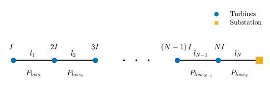
Figure 10.
Power losses in a cable branch.
Accordingly, the total of power losses in a cable branch is calculated by the Equation (21) [22]:
where and are the length and the conductor resistance of the i-th cable section, respectively.
4.4. Optimization with Particle Swarm Algorithm
Particle Swarm Optimization is a metaheuristic optimization was developed by R. Eberhardt and J. Kennedy [23], which consists of a group of individuals that are influenced by simple communicative processes within their neighborhood. The swarm and its emergence are no longer used to simulate the flight of birds, but to determine the optimum of a fitness function. In [24], Kennedy and Eberhardt explain a model that fundamentally describes swarm intelligence based on three simple operations. They include the adaptation in a population and thus optimization as the result of the evaluation, comparison and imitation. They consider the swarm in terms of two components; the ”low-level” component, which describes the behavior and communicative processes of the individuals and the resulting “high-level” component, which describes the complex structures and orders, in this case, the emergent resulting strategy to find an optimum.
Evaluation is the prerequisite for every goal-oriented action because without the possibility to evaluate the current state, it is not possible to act in the sense of improvement. The comparison is the second important operation. Thus, more highly developed life forms are not only able to compare their current state with historical states, but through communication can also use the knowledge of other individuals and compare it with their own. The imitation is the third operation, meaning that living beings now draw conclusions from the evaluation and the comparison by imitating “good behavior”.
The Particle Swarm Optimization applies these three operations to a particle swarm so as to use the resulting emergent effect for optimization. Considering the swarm as a natural swarm of birds or fish moving at certain speeds, each particle is modeled by its position within the search space and by its velocity. All particles continuously adjust their positions and their velocities, accordingly their trajectories with regard to the best positions, on the particle with the best position within the swarm and on their current position. In fact, each particle is influenced not only by its own experience but also by that of other particles in the swarm. The position of each particle during a particular iteration to its previous position is expressed in Equation (22) [23]:
where the velocity is given by Equation (23) [25]:
where , , , and are coefficients defining the weighting of the various contributors determined by tuning the Particle Swarm Optimization to the present optimization problem, p is the best position of the relevant particle, g is the best position of the swarm and is a random number [23,25]. The main approach of Particle Swarm Optimization is shown in Figure 11.
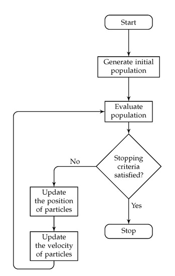
Figure 11.
Flowchart of the Particle Swam Optimization Algorithm.
4.5. Regular and Irregular Wind Farms
For the verification of the optimization approach, some assumptions were taken into account in regular as well as in irregular wind farms. The minimum distance between all turbines is 1 . The feeders are in a radial structure. The substation is outside the turbine array. The calculated inter-array cable lengths for the power collection system for regular and irregular wind farms are and , respectively. A swarm size of 3 was used for the optimization because of the simplicity of the optimization problem.
After optimization of the objective function in Equation (19) using the Particle Swarm Algorithm, by minimizing the Euclidean distance from the substation to each of the turbines, the total length of the inter-array cables after new cable laying is and , which means a saving in cable length of and respectively. The average computation time for the optimization in both cases is . It can be concluded that the optimal position of the substation is in the middle of the wind farm. The initial locations of the substations for regular and irregular wind farms, the results of the optimization and the convergence curves are shown in Figure 12 and Figure 13.
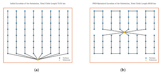
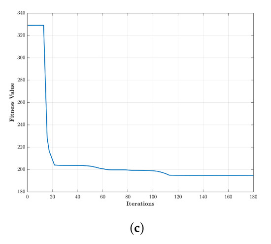
Figure 12.
Initial and optimized substation location in a regular wind farm: (a) Initial substation location. (b) Optimized substation location. (c) Convergence curve.
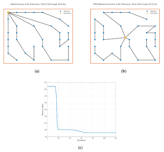
Figure 13.
Initial and optimized substation location in an irregular wind farm: (a) Initial substation location. (b) Optimized substation location. (c) Convergence curve.
4.6. Real Case Study (Horns Rev 1)
The offshore wind farm Horns Rev 1 consisting of 80 wind turbines was built off the coast of Denmark on the area of 20 2 and has been in operation since the end of 2002. The collector topology is radial and the substation is located outside the turbine array, therefore it is a suitable example to verify and demonstrate the reliability of the optimization approach. More data about this wind farm is in Table 2 [25].
Table 2.
Specifications of Horns Rev 1.
For this case study, the presumed total cable length for the power collection system is . In reality, the length of the cable topology is 63 . Interesting results are provided after optimizing the substation location using Particle Swarm Optimization. However, it is first assumed that the transformer station can tolerate an additional cable entry to avoid crossing of submarine cables. Thus, the cable entries are 6 instead of 5 in the initial situation. Figure 14 shows the initial state, the proposed cable routing after optimizing the transformer station location and the convergence curve.
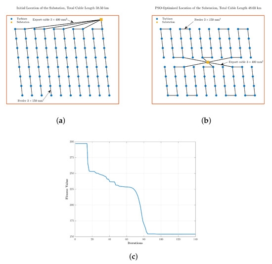
Figure 14.
Initial and optimized substation location in Horns Rev 1: (a) Initial substation location. (b) Optimized substation location. (c) Convergence curve.
The saved cable length is , which means of the initial total cable length. The collector topology of Horns Rev 1 comprises two types of AC cable. For the feeders between the wind turbines, a cross-linked polyethylene submarine cable (XLPE) with a cross-section of 2 is used, while a cross-section of 2 for the export cable between the connection wind turbine to the substation is employed. The estimated prices for the two types of cables are 130 €/ and 230 €/. Meanwhile, the cost of installation by a vessel is estimated to be 250 €/, regardless of the cable type. Table 3 shows the economic benefits of optimization of the substation location in the offshore wind farm Horns Rev 1, which are about .
Table 3.
Economic benefits of the optimization approach for the Horns Rev 1.
The Equation (21) can be used to make technical analysis and calculation of the power losses in the AC submarine cables. This is done by using the conductor resistance of the cable and the outgoing electrical current from the 2 wind turbine, which is approximately 33 [26]. Assuming that the wind farm is in continuous operation, the power losses in the entire collector topology could be reduced by approximately by optimizing the substation location compared to the initial layout. The results are shown in Table 4, where and are the power losses for one year and 25 years, respectively.
Table 4.
Technical benefits of the optimization approach for the Horns Rev 1.
5. Optimization of the Collector Topology
5.1. Multiple Traveling Salesmen Problem
The Multiple Traveling Salesmen Problem is considered to be a special case of the classical Traveling Salesman Problem. According to the classification of the Traveling Salesman Problem as an NP-hard problem, the Multiple Traveling Salesmen Problem is more difficult than the classical variant [27,28,29]. The Traveling Salesman Problem is a typical combinatorial optimization problem [30] and is generally defined such that a salesman starts his travel from a starting node and returns after visiting n nodes, so that every node is visited only once. The main objective is to find the shortest minimum cycle with the minimum cost. In the case of Multiple Traveling Salesmen Problem, several salesmen are assigned to given nodes, so that each node is visited only once by exactly one salesman, except for the common starting point. Accordingly, the routes have a loop shape. This type of Multiple Traveling Salesmen Problem is known as a single depot returning Multiple Traveling Salesmen Problem and can be used to optimize the collector system of a wind farm with ring topology, where the depot or starting point can be considered to be a substation and the nodes as wind turbines. In the case of the radial topology of the collector system, another variant of the Multiple Traveling Salesmen Problem is chosen for the optimization, which is known as single depot non-returning Multiple Traveling Salesmen Problem.
The first variant of the Multiple Traveling Salesmen Problem for ring wind farm topology is well described in [31] and is also presented here. For the problem formulation a set of nodes locations is denoted by , where is the number of nodes. The location of the depot is defined by and the square Euclidean distance between two nodes i and j is determined by . A tour which is equivalent to the cable routing in a wind farm, is denoted by the sequence or depending on whether the start and end points coincide or not, where defines the i-th node in a tour. Notice that when and and that .
For a given number m of salesmen, the objective function for the single depot returning Multiple Traveling Salesmen Problem can be described mathematically like in Equation (24) [31]:
Removal of edge is serving to separate the route between two salesmen j and , while adding of edges and guarantees that the tour for salesman j ends at the depot and the tour for salesman starts at the depot. The quantity if the edge corresponding to the nodes is removed.
5.2. Genetic Algorithm
Genetic Algorithms, also known as Evolutionary Algorithms, are inspired by Charles Darwin’s concept of natural evolution, which is the optimization of individuals competing against each other for resources [32]. Some individuals are better suited for this; therefore, they have a greater chance of survival and can pass their traits on to offspring, others not. These traits are defined in the genome. A single parameter that describes a trait is called a gene. A whole set of such genes is a chromosome. The concept of the Genetic Algorithm was developed in 1975 by John Holland to describe adaptive systems [33]. The strength of the Genetic Algorithm is its ability to find solutions even for very complex optimization problems where other search methods fail. It is characterized by its variability so that it can be adapted to many problems. Genetic Algorithm is based on a population of individuals who, by means of the genetic operations “selection” and ”variation”, produce offspring that are better suited to solve the optimization problem than their parents.
The selection gives the Genetic Algorithm the direction in the search space, by favoring good individuals for reproduction and avoiding bad ones. The resulting loss of diversity in the population will be counteracted using the variation operators “crossover” and ”mutation” by developing new solutions from the existing ones. The new generation of individuals will be selected from the existing individuals in a population depending on their fitness. The new generation is then inserted into the new population after operating of the crossover and mutation with the rates and , respectively. The main task of crossover is the recombination of two individuals and the creation of two new ones, while the mutation is used to prevent the Genetic Algorithm from “sticking” to a local optimum. Figure 15 illustrates the crossover and the mutation of a chromosome.
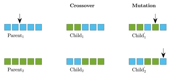
Figure 15.
Crossover and mutation.
As abort criteria, the reaching of the maximum number of iterations, the maximum computing time or the convergence in the search space are often used. The algorithm offers a broad applicability and is therefore also suitable for complex search spaces. There are also no restrictive requirements for the objective function, which can be continuous as well as a discrete function. The flowchart in Figure 16 shows the main steps of the Genetic Algorithm.
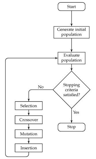
Figure 16.
Flowchart of the Genetic Algorithm.
5.3. Optimization of Ring Collector Topology
In order to verify the reliability of the optimization approach using the combination between the Genetic Algorithm and the single depot returning Multiple Traveling Salesmen Problem, 32 locations of wind turbines, with a minimum distance of 560 between them, are randomly generated. Figure 17 shows the created wind farm and its optimized ring collector system. The optimization converges within approximately 5 with a total cable length of .
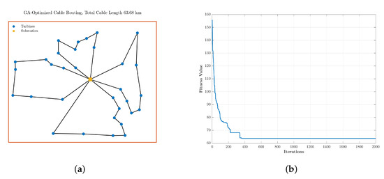
Figure 17.
Optimized cable routing for the ring collector topology: (a) Optimized cable routing. (b) Convergence curve.
5.4. Optimization of Radial Collector Topology
For the optimizing of the radial collector topology with the proposed optimization approach, using the combination between the Genetic Algorithm and single depot non-returning Multiple Traveling Salesmen Problem, the wind farm with already optimized substation location in Figure 13b will be used to see if further savings can be made on the overall cable length of the grid network. The length of the inter-array cable of the wind farm has been reduced by an additional , representing approximately compared to the state shown in Figure 13b. Figure 18 shows the optimized cable routing and the associated convergence curve for a radial collector topology.
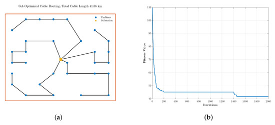
Figure 18.
Optimized cable routing for a radial collector topology: (a) Optimized cable routing. (b) Convergence curve.
The optimization approach is in addition evaluated on two real existing offshore wind farms, Westermost Rough offshore wind farm in England and Luchterduinen offshore wind farm in the Netherlands, both located in the North Sea and whose collector topology are laid out as a string structure. Further specifications are listed in the Table 5.
Table 5.
Specifications of Westermost Rough and Luchterduinen offshore wind farms.
Regardless of the cable types, the routing of the inter-array cable for both offshore wind farms will be optimized with the suggested combination of the Genetic Algorithm and the single depot non-returning Multiple Traveling Salesmen Problem. Figure 19 and Figure 20 show the initial cable layouts, the results of the applied optimization on both offshore wind farms and the corresponding convergence curves.
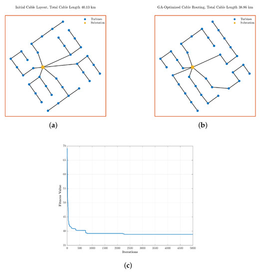
Figure 19.
Initial and optimized cable routing for Westermost Rough offshore wind farm: (a) Initial cable routing. (b) Optimized cable routing. (c) Convergence curve.
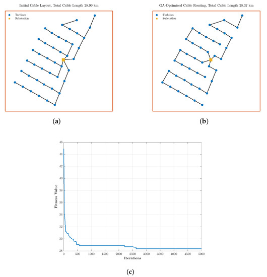
Figure 20.
Initial and optimized cable routing for Luchterduinen offshore wind farm: (a) Initial cable routing. (b) Optimized cable routing. (c) Convergence curve.
In the Westermost Rough offshore wind farm, a minimization of the cable length of exactly was achieved, corresponding to . Meanwhile, in the Luchterduinen offshore wind farm, a reduction of only was obtained, representing approximately of the total cable length of the collector topology.
6. Conclusions and Future Work
In this paper, the authors presented the procedure for mastering an optimal design of a wind farm layout and its optimal collector topology using metaheuristic algorithms. In the beginning, the method of estimating the annual energy production before the design phase of a wind farm by evaluating meteorological measurements at the located site and at the desired altitude was introduced.
The second part of this paper focuses on the model for the problem of wind turbine positioning, which is based on the Jensen model. The parameters used for the optimization approach using the Simulated Annealing Algorithm are constant. The optimization shows an improvement in cost per unit generated power of the wind farm compared to the initial solution. The minimizing of this objective function also means maximization of the power production. For the extension of this work, the optimization of a wind farm with wind turbines of different hub heights, with variable wind speeds as well as with variable wind directions can be performed. However, the optimal design of the wind farm becomes particularly complex due to the variable parameters of the optimization problem.
After optimization of the wind turbine position within a given wind farm area, the authors also presented the optimization of the substation location using the Particle Swarm Algorithm. The optimization approach was performed on both regular and irregular wind farm and showed good results regarding the savings in cable length of the wind farm collector system. The optimal positioning of the substation is in the middle of the wind farm. The approach was also run on a real existing offshore wind farm and a comparison between the initial and optimized state was made. The study showed both the economic and technical advantages. The economic benefit means savings in the total investment costs, while the technical advantages are the minimization of cable power losses by minimizing the total cable length of the collector system.
The last part of the article is dedicated to optimizing the routing of inter-array cables within a wind farm. The grid network includes feeders between the wind turbines and export cables from the turbines to the substation. The optimization approach is based on the combination of the Genetic Algorithm and the single depot Multiple Traveling Salesmen Problem. In order to verify the reliability of the approach, the optimization was performed on two randomly generated wind farms with both ring and radial topology. Very good results were obtained regarding the minimization of the total cable length of the collector system, which also means savings in total investment costs as well as minimization of cable power losses. The optimization approach was additionally applied to two real existing offshore wind farms and the reliability was proven. As an extension of this optimization approach of the cable routing into the grid network, the selection of the suitable cable cross-section for the feeders and the export cables can be further enhanced.
All of these optimization approaches can already be implemented in the design phase and thus, both the total investment costs and the costs incurred, e.g., cable power losses, can be minimized over the lifetime of the wind farm.
Author Contributions
Conceptualization, C.E.M. and A.A.; methodology, C.E.M.; software, C.E.M.; validation, A.A. All authors have read and agreed to the published version of the manuscript.
Funding
This research received no external funding.
Conflicts of Interest
The authors declare no conflict of interest.
References
- Rabiul Islam, M.; Guo, Y.; Zhu, J. A review of offshore wind turbine nacelle: Technical challenges, and research and developmental trends. Renew. Sustain. Energy Rev. 2014, 33, 161–176. [Google Scholar] [CrossRef]
- Gao, X.; Yang, H.; Lu, L.; Koo, P. Wind turbine layout optimization using multi-population genetic algorithm and a case study in Hong Kong offshore. J. Wind Eng. Ind. Aerodyn. 2015, 139, 89–99. [Google Scholar] [CrossRef]
- Wu, X.; Hu, W.; Huang, Q.; Chen, C.; Chen, Z.; Blaabjerg, F. Optimized Placement of Onshore Wind Farms Considering Topography. Energies 2019, 12, 2944. [Google Scholar] [CrossRef]
- González, J.S.; Payán, M.B.; Santos, J.R. A New and Efficient Method for Optimal Design of Large Offshore Wind Power Plants. IEEE Trans. Power Syst. 2013, 28, 3075–3084. [Google Scholar] [CrossRef]
- Fischetti, M.; Pisinger, D. Optimizing wind farm cable routing considering power losses. Eur. J. Oper. Res. 2018, 270, 917–930. [Google Scholar] [CrossRef]
- Feng, J.; Shen, W.Z. Modelling Wind for Wind Farm Layout Optimization Using Joint Distribution of Wind Speed and Wind Direction. Energies 2015, 8, 3075–3092. [Google Scholar] [CrossRef]
- Larsen, G.C. A Simple Wake Calculation Procedure, 1st ed.; Risø National Laboratory: Roskilde, Denmark, 1988; ISBN 87-550-1484-4. [Google Scholar]
- Frandsen, S.; Barthelmie, R.; Pryor, S.; Rathmann, O.; Larsen, S.; Hojstrup, J.; Thogersen, M. Analytical modelling of wind speed deficit in large offshore wind farms. Wind Energy 2006, 9, 39–53. [Google Scholar] [CrossRef]
- Ainslie, J.F. Calculating the flowfield in the wake of wind turbines. J. Wind Eng. Ind. Aerodyn. 1988, 27, 213–224. [Google Scholar] [CrossRef]
- Jensen, N.O. A Note on Wind Generator Interaction, 1st ed.; Risø National Laboratory: Roskilde, Denmark, 1983; ISBN 87-550-0971-9. [Google Scholar]
- Chen, Y.; Li, H.; Jin, K.; Song, Q. Wind farm layout optimization using genetic algorithm with different hub height wind turbines. Energy Convers. Manag. 2013, 70, 56–65. [Google Scholar] [CrossRef]
- Beskirli, M.; Koç, I.; Kodaz, H. Optimal Placement of Wind Turbines Using Novel Binary Invasive Weed Optimization. Teh. Vjesn. 2019, 26, 56–63. [Google Scholar] [CrossRef]
- Jiang, J.N.; Tang, C.Y.; Ramakumar, R.G. Control and Operation of Grid-Connected Wind Farms; Springer: Berlin, Germany, 2016; ISBN 978-3-319-39135-9. [Google Scholar]
- Mosetti, G.; Poloni, C.; Diviacco, B. Optimization of wind turbine positioning in large wind farms by means of a genetic algorithm. J. Wind Eng. Ind. Aerodyn. 1994, 51, 105–116. [Google Scholar] [CrossRef]
- Hachimi, H. Hybridations D’Algorithmes MéTaheuristiques en Optimisation Globale Et Leurs Applications; HAL Archives: Lyon, France, 2013. [Google Scholar]
- Černý, V. Thermodynamical approach to the traveling saleman problem: An efficient simulation algorithm. J. Optim. Theory Appl. 1985, 45, 41–51. [Google Scholar] [CrossRef]
- Kirkpatrick, S.; Gelatt, C.; Vecchi, M.P. Optimization by simulated annealing. Science 1983, 220, 671–680. [Google Scholar] [CrossRef] [PubMed]
- Pérez-Rúa, J.A.; Stolpe, M.; Das, K.; Cutululis, N.A. Global Optimization of Offshore Wind Farm Collection Systems. IEEE Trans. Power Syst. 2020, 35, 2256–2267. [Google Scholar] [CrossRef]
- Rabiul Islam, M.; Guo, Y.; Zhu, J.; Lu, H.; Jin, J. High-Frequency Magnetic-Link Medium-Voltage Converter for Superconducting Generator-Based High-Power Density Wind Generation Systems. IEEE Trans. Appl. Supercond. 2014, 24, 1–5. [Google Scholar] [CrossRef]
- Rabiul Islam, M.; Ashib Rahman, M.; Muttaqi, K.; Sutanto, D. A New Magnetic-Linked Converter for Grid Integration of Offshore Wind Turbines Through MVDC Transmission. IEEE Trans. Appl. Supercond. 2019, 29, 1–5. [Google Scholar] [CrossRef]
- Madariaga, A.; Martín, J.; Zamora, I.; Ceballos, S.; Anaya-Lara, O. Effective Assessment of Electric Power Losses in Three-Core XLPE Cables. IEEE Trans. Power Syst. 2013, 28, 4488–4495. [Google Scholar] [CrossRef]
- Fischetti, M.; Pisinger, D. On the Impact of Considering Power Losses in Offshore Wind Farm Cable Routing. Eur. J. Oper. Res. 2018, 270, 917–930. [Google Scholar] [CrossRef]
- Kiranyaz, S.; Ince, T.; Gabbouj, M. Multidimensional Particle Swarm Optimization for Machine Learning and Pattern Recognition, 1st ed.; Springer: Berlin, Germany, 2014; ISBN 978-3-642-37846-1. [Google Scholar]
- Kennedy, J.; Eberhart, R.C.; Shi, Y. Swarm Intelligence; Morgan Kaufmann: Burlington, NJ, USA, 2001; ISBN 978-1-558-60595-4. [Google Scholar]
- El Mokhi, C.; Addaim, A. Optimal Substation Location Of A Wind Farm Using Different Metaheuristic Algorithms. In Proceedings of the 6th IEEE International Conference on Optimization and Applications (ICOA2020), Beni Mellal, Morocco, 20–21 April 2020; pp. 1–6. [Google Scholar]
- Srikakulapu, R.; Urundady, V. Combined approach based on ACO with MTSP for optimal internal electrical system design of large offshore wind farm. In Proceedings of the International Conference on Power, Instrumentation, Control and Computing (PICC2018), Thrissur, India, 18–20 January 2018; pp. 1–6. [Google Scholar]
- Kencana, E.N.; Harini, I.; Mayuliana, K. The Performance of Ant System in Solving Multi Traveling Salesmen Problem. In Proceedings of the 4th Information Systems International Conference (ISIC2017), Bali, Indonesia, 6–8 November 2017; pp. 46–52. [Google Scholar]
- Larki, H.; Yousefikhoshbakht, M. Solving the multiple traveling salesman problem by a novel meta-heuristic algorithm. J. Optim. Ind. Eng. 2014, 7, 55–63. [Google Scholar]
- Hou, M.; Liu, D. A novel method for solving the multiple traveling salesmen problem with multiple depots. Chin. Sci. Bull. 2012, 57, 1886–1892. [Google Scholar] [CrossRef][Green Version]
- Pan, L.; Paun, G.; Pérez-Jiménez, M.J.; Song, T. Bio-Inspired Computing—Theories and Applications, 9th ed.; Springer Science and Business Media LLC: New York, NY, USA, 2014; ISBN 978-3-662-45049-9. [Google Scholar]
- Baranwal, M.; Roehl, B.; Salapaka, S.M. Multiple traveling salesmen and related problems: A maximum-entropy principle based approach. In Proceedings of the American Control Conference (ACC2017), Seattle, WA, USA, 24–26 May 2017; pp. 3944–3949. [Google Scholar]
- Ellaia, R.; Hachimi, H.; ELHami, A. A New Hybrid Genetic Algorithm and Particle Swarm Optimization. Key Eng. Mater. 2012, 498, 115–125. [Google Scholar] [CrossRef]
- Holland, J.H. Adaptation in Natural and Artificial Systems: An Introductory Analysis with Applications to Biology, Control, and Artificial Intelligence; MIT Press: Cambridge, MA, USA, 1992; ISBN 978-0-262-58111-0. [Google Scholar]
© 2020 by the authors. Licensee MDPI, Basel, Switzerland. This article is an open access article distributed under the terms and conditions of the Creative Commons Attribution (CC BY) license (http://creativecommons.org/licenses/by/4.0/).