Towards a Comprehensive Framework of the Relationships between Resource Footprints, Quality of Life, and Economic Development


Abstract
1. Introduction
2. Materials and Methods
3. Results
3.1. Regression Analysis
3.2. Timeline Analysis
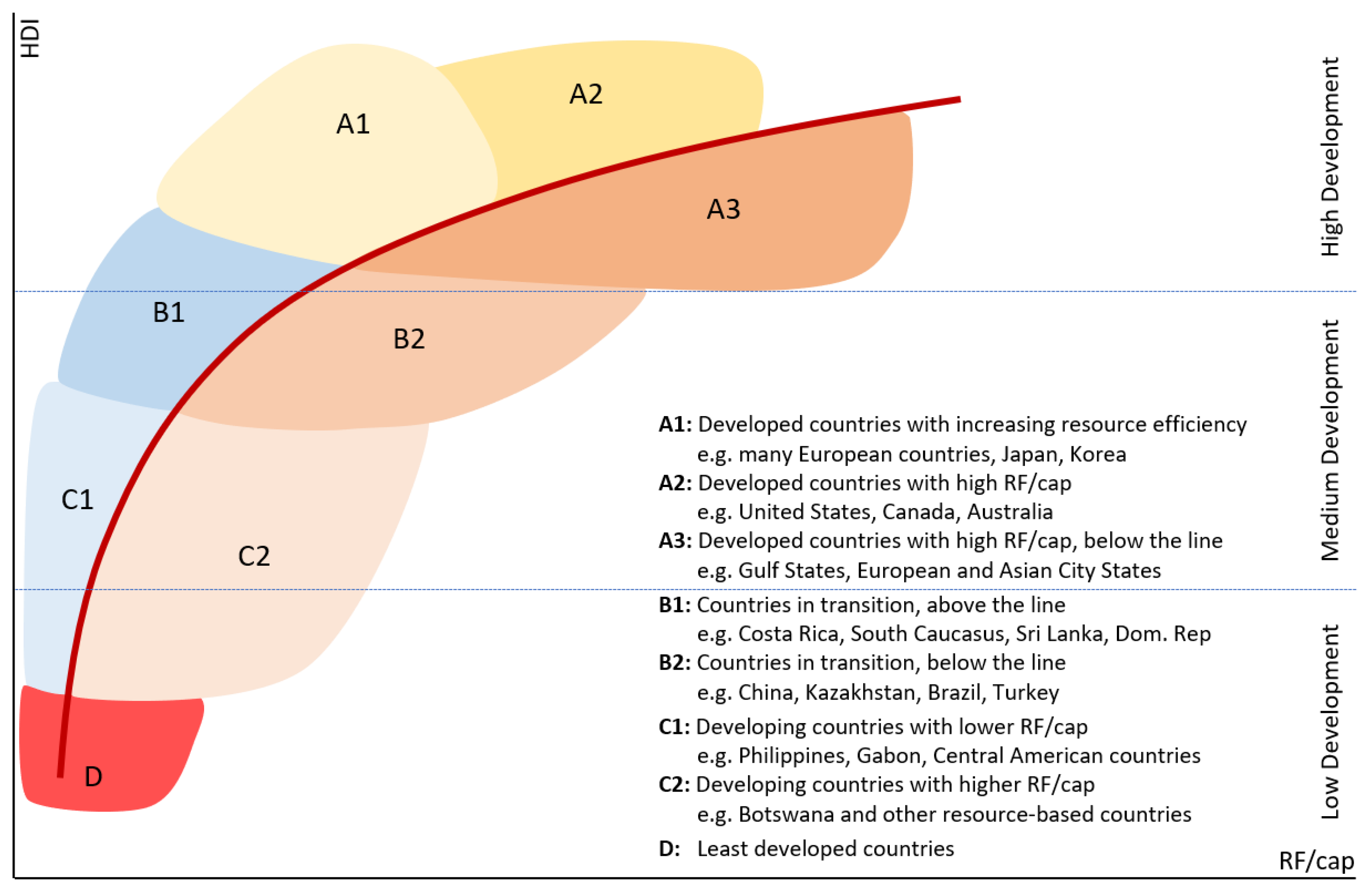
3.3. Deriving Development Clusters
4. Discussion
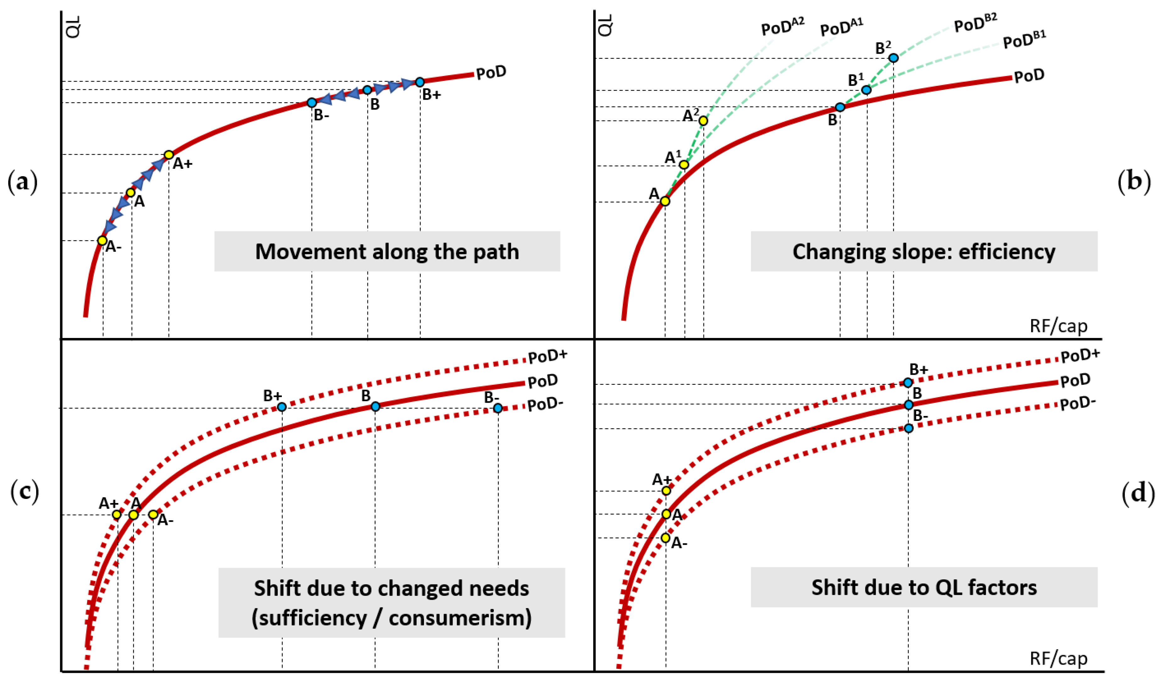
4.1. Properties of the Path of Development
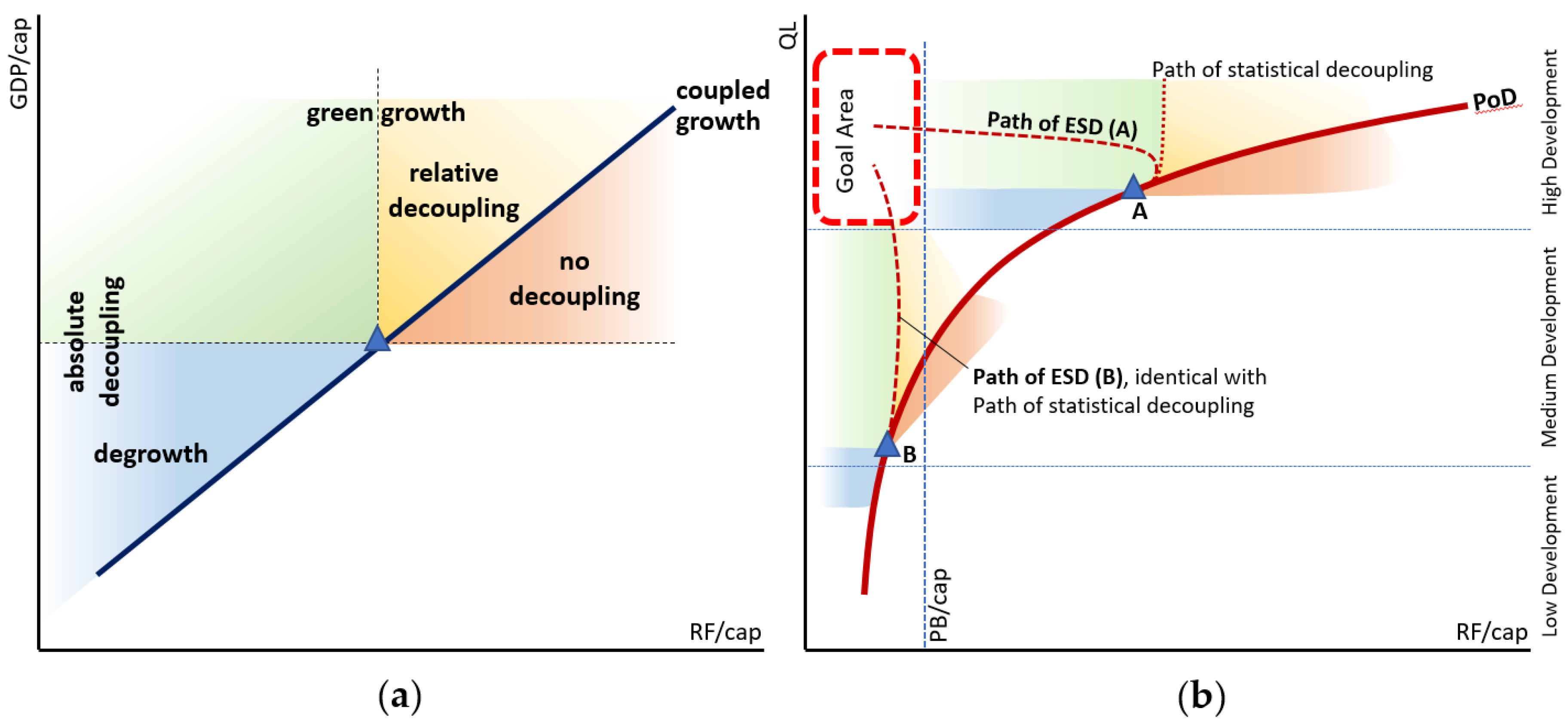
4.2. Planetary and Social Boundaries and Their Implications for Decoupling
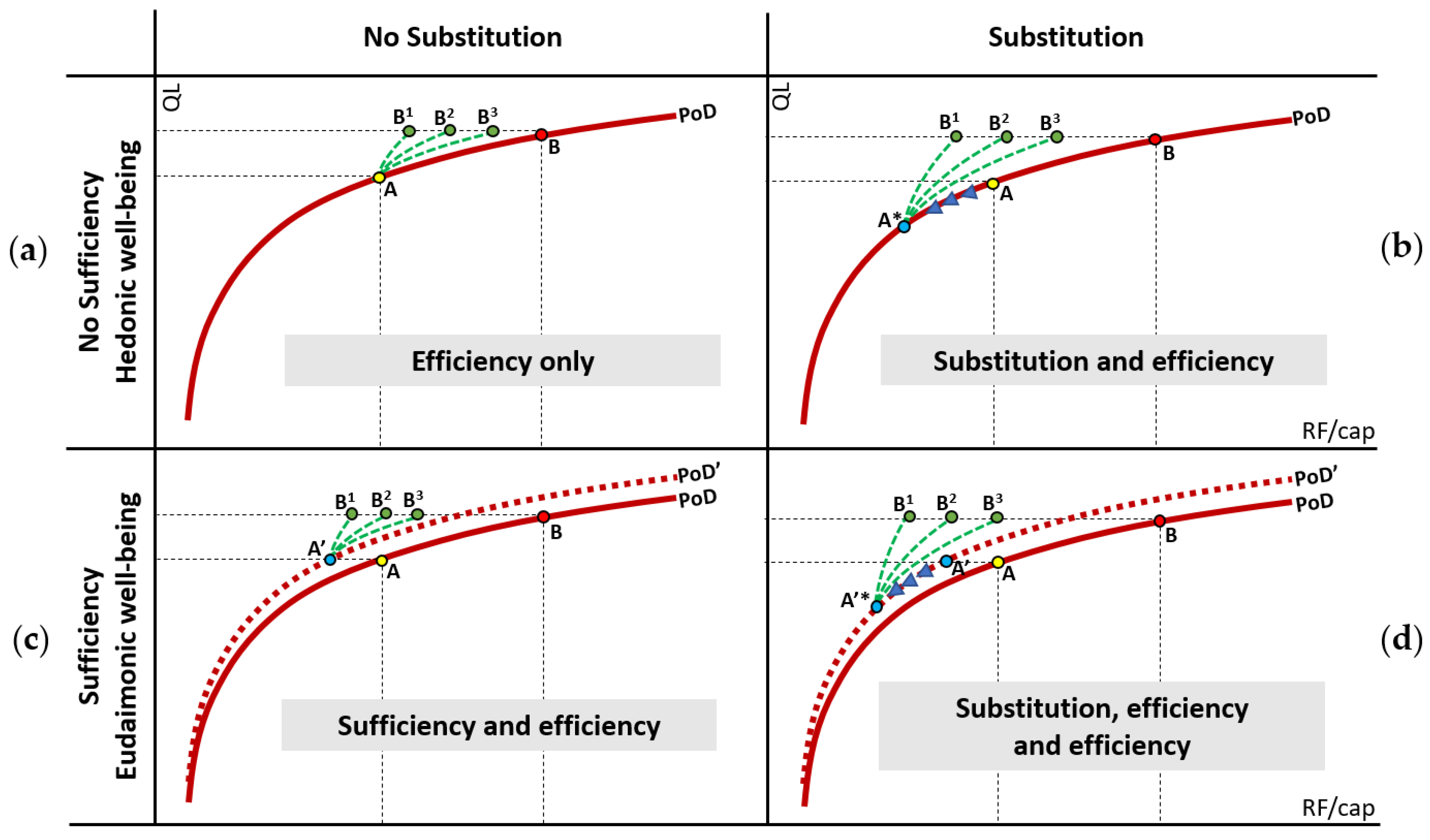
4.3. Options to Reach the Goal Area
4.4. The Relationship to Economic Growth Models
5. Conclusions
Supplementary Materials
Author Contributions
Funding
Acknowledgments
Conflicts of Interest
References
- Illge, L.; Schwarze, R. A matter of opinion—How ecological and neoclassical environmental economists and think about sustainability and economics. Ecol. Econ. 2009, 68, 594–604. [Google Scholar] [CrossRef]
- Hanley, N.; Shogren, J.F.; White, B. Environmental Economics in Theory and Practice, 2nd ed.; Palgrave Macmillan: Basingstoke, UK, 2007; ISBN 9780333971376 033397137x. [Google Scholar]
- Stiglitz, J.E. A Neoclassical Analysis of the Economics of Natural Resources; Working Paper No. R0077. ssrn.com/abstract=250334; NBER: Cambridge, MA, USA, 1980. [Google Scholar]
- Common, M.; Perrings, C. Towards and ecological economics of sustainability. Ecol. Econ. 1992, 6, 7–34. [Google Scholar] [CrossRef]
- Daly, H.E. Georgescu-Roegen versus Solow/Stiglitz. Ecol. Econ. 1997, 22, 261–266. [Google Scholar] [CrossRef]
- Steffen, W.; Richardson, K.; Rockström, J.; Cornell, S.E.; Fetzer, I.; Bennett, E.M.; Biggs, R.; Carpenter, S.R.; de Vries, W.; de Wit, C.A.; et al. Planetary boundaries: Guiding human development on a changing planet. Science 2015, 347, 1259855. [Google Scholar] [CrossRef] [PubMed]
- Raworth, K. A safe and just space for humanity. Oxfam Policy Pract. Clim. Change Resil. 2012, 8, 1–26. [Google Scholar]
- UNEP. Decoupling Natural Resource Use and Environmental Impacts from Economic Growth. A Report of the Working Group on Decoupling to the International Resource Panel; Fischer-Kowalski, M., Swilling, M., von Weizsäcker, E.U., Ren, Y., Moriguchi, Y., Crane, W., Krausmann, F., Eisenmenger, N., Giljum, S., Hennicke, P., et al., Eds.; UNEP: Nairobi, Kenya, 2011. [Google Scholar]
- van den Bergh, J.C.J.M.; Kallis, G. Growth, A-Growth or Degrowth to Stay within Planetary Boundaries? J. Econ. Issues 2012, 46, 909–920. [Google Scholar] [CrossRef]
- Jackson, T. Prosperity without Growth. Economics for a Finite Planet; Earthscan: London, UK, 2009; ISBN 9781844078943 (hbk.) 1844078949 (hbk.). [Google Scholar]
- Meadows, D.H.; Meadows, D.J.; Randers, J.; Behrens, W.W. The Limits to Growth. A Report for the Club of Rome’s Project on the Predicament of Mankind; Universe Books: New York, NY, USA, 1972; ISBN 0876631650. [Google Scholar]
- Hardt, L.; O’Neill, D.W. Ecological Macroeconomic Models: Assessing Current Developments. Ecol. Econ. 2017, 134, 198–211. [Google Scholar] [CrossRef]
- Brand-Correa, L.I.; Steinberger, J.K. A Framework for Decoupling Human Need Satisfaction From Energy Use. Ecol. Econ. 2017, 141, 43–52. [Google Scholar] [CrossRef]
- Mayer, A.; Haas, W.; Wiedenhofer, D.; Krausmann, F.; Nuss, P.; Blengini, G.A. Measuring Progress towards a Circular Economy: A Monitoring Framework for Economy-wide Material Loop Closing in the EU28. J. Ind. Ecol. 2018, 132, 1. [Google Scholar] [CrossRef] [PubMed]
- Geiger, S.M.; Fischer, D.; Schrader, U. Measuring What Matters in Sustainable Consumption: An Integrative Framework for the Selection of Relevant Behaviors. Sustain. Dev. 2018, 26, 18–33. [Google Scholar] [CrossRef]
- Kirchherr, J.; Reike, D.; Hekkert, M. Conceptualizing the circular economy: An analysis of 114 definitions. Resour. Conserv. Recycl. 2017, 127, 221–232. [Google Scholar] [CrossRef]
- Korhonen, J.; Honkasalo, A.; Seppälä, J. Circular Economy: The Concept and its Limitations. Ecol. Econ. 2018, 143, 37–46. [Google Scholar] [CrossRef]
- Tukker, A.; Ekins, P. Concepts Fostering Resource Efficiency: A Trade-off between Ambitions and Viability. Ecol. Econ. 2019, 155, 36–45. [Google Scholar] [CrossRef]
- Dietz, T.; Rosa, E.A.; York, R. Environmentally Efficient Well-Being: Rethinking Sustainability as the Relationship between Human Well-being and Environmental Impacts. Hum. Ecol. Rev. 2009, 16, 114–123. [Google Scholar]
- Jorgenson, A.K.; Dietz, T. Economic growth does not reduce the ecological intensity of human well-being. Sustain. Sci. 2015, 10, 149–156. [Google Scholar] [CrossRef]
- Zhang, S.; Zhu, D.; Shi, Q.; Cheng, M. Which countries are more ecologically efficient in improving human well-being? An application of the Index of Ecological Well-being Performance. Resour. Conserv. Recycl. 2018, 129, 112–119. [Google Scholar] [CrossRef]
- Mazur, A.; Rosa, E. Energy and Life-Style. Science 1974, 186, 607–610. [Google Scholar] [CrossRef] [PubMed]
- Steinberger, J.K.; Roberts, J.T. From constraint to sufficiency: The decoupling of energy and carbon from human needs, 1975–2005. Ecol. Econ. 2010, 70, 425–433. [Google Scholar] [CrossRef]
- Lamb, W.F.; Rao, N.D. Human development in a climate-constrained world: What the past says about the future. Glob. Environ. Change 2015, 33, 14–22. [Google Scholar] [CrossRef]
- Pasternak, A.D. Global Energy Futures and Human Development: A Framework for Analysis; US Department of Energy: Oak Ridge, TN, USA, 2000.
- Dittrich, M.; Giljum, S.; Lutter, S.; Polzin, C. Green Economies around the World? The Role of Resource Use for Development and the Environment; SERI: Vienna, Austria, 2012. [Google Scholar]
- Giljum, S.; Dittrich, M.; Lieber, M.; Lutter, S. Global patterns of material flows and their socio-economic and environmental implications: A MFA study on all countries world-wide from 1980 to 2009. Resources 2014, 3, 319–339. [Google Scholar] [CrossRef]
- Moran, D.D.; Wackernagel, M.; Kitzes, J.A.; Goldfinger, S.H.; Boutaud, A. Measuring sustainable development—Nation by nation. Ecol. Econ. 2008, 64, 470–474. [Google Scholar] [CrossRef]
- Kassouri, Y.; Altıntaş, H. Human well-being versus ecological footprint in MENA countries: A trade-off? J. Environ. Manag. 2020, 263, 110405. [Google Scholar] [CrossRef] [PubMed]
- Wackernagel, M.; Rees, W.E. Perceptual and structural barriers to investing in natural capital: Economics from an ecological footprint perspective. Ecol. Econ. 1997, 20, 3–24. [Google Scholar] [CrossRef]
- Tukker, A.; Bulavskaya, T.; Giljum, S.; Koning, A.D.; Lutter, S.; Simas, M.; Stadler, K.; Wood, R. Environmental and resource footprints in a global context: Europe’s structural deficit in resource endowments. Glob. Environ. Chang. 2016, 40, 171–181. [Google Scholar] [CrossRef]
- Vita, G.; Hertwich, E.; Stadler, K.; Wood, R. Connecting global emissions to fundamental human needs and their satisfaction. Environ. Res. Lett. 2019, 14, 14002. [Google Scholar] [CrossRef]
- Ambrey, C.L.; Daniels, P. Happiness and footprints: Assessing the relationship between individual well-being and carbon footprints. Environ. Dev. Sustain. 2017, 19, 895–920. [Google Scholar] [CrossRef]
- Steinberger, J.K.; Lamb, W.F.; Sakai, M. Your money or your life? The carbon-development paradox. Environ. Res. Lett. 2020, 15, 44016. [Google Scholar] [CrossRef]
- Fanning, A.L.; O’Neill, D.W. The Wellbeing–Consumption paradox: Happiness, health, income, and carbon emissions in growing versus non-growing economies. J. Clean. Prod. 2019, 212, 810–821. [Google Scholar] [CrossRef]
- Juknys, R.; Liobikienė, G.; Dagiliūtė, R. Deceleration of economic growth - The main course seeking sustainability in developed countries. J. Clean. Prod. 2018, 192, 1–8. [Google Scholar] [CrossRef]
- Kalimeris, P.; Bithas, K.; Richardson, C.; Nijkamp, P. Hidden linkages between resources and economy: A “Beyond-GDP” approach using alternative welfare indicators. Ecol. Econ. 2020, 169, 106508. [Google Scholar] [CrossRef]
- O’Neill, D.W.; Fanning, A.L.; Lamb, W.F.; Steinberger, J.K. A good life for all within planetary boundaries. Nat. Sustain. 2018, 1, 88–95. [Google Scholar] [CrossRef]
- Rockström, J.; Steffen, W.; Noone, K.; Persson, A.; Chapin, F.S.; Lambin, E.F.; Lenton, T.M.; Scheffer, M.; Folke, C.; Schellnhuber, H.J.; et al. A safe operating space for humanity. Nature 2009, 461, 472. [Google Scholar] [CrossRef] [PubMed]
- Stoknes, P.E.; Rockström, J. Redefining green growth within planetary boundaries. Energy Res. Soc. Sci. 2018, 44, 41–49. [Google Scholar] [CrossRef]
- Parrique, T.; Barth, J.; Briens, F.; Kerschner, C.; Kraus-Polk, A.; Kuokkanen, A.; Spangenberg, J.H. Decoupling Debunked: Evidence and Arguments against Green Growth as a Sole Strategy for Sustainability; European Environmental Bureau: Brussels, Belgium, 2019. [Google Scholar]
- Randers, J.; Rockstroem, J.; Stoknes, P.E.; Golüke, U.; Collste, D.; Cornell, S. Transformation is feasible. How to achieve the Sustainable Development Goals within Planetary Boundaries. Report to the Club of Rome; Stockholm Resilience Centre, Stockholm University, Norwegian Business School, Global Challenges Foundation: Stockholm, Sweden, 2018. [Google Scholar]
- Amos, R.; Lydgate, E. Trade, transboundary impacts and the implementation of SDG 12. Sustain. Sci. 2019. [Google Scholar] [CrossRef]
- Steffen, W.; Rockström, J.; Richardson, K.; Lenton, T.M.; Folke, C.; Liverman, D.; Summerhayes, C.P.; Barnosky, A.D.; Cornell, S.E.; Crucifix, M.; et al. Trajectories of the Earth System in the Anthropocene. Proc. Natl. Acad. Sci. USA 2018, 115, 8252–8259. [Google Scholar] [CrossRef] [PubMed]
- IPCC. Global Warming of 1.5 °C. An IPCC Special Report on the Impacts of Global Warming of 1.5 °C above Pre-industrial Levels and Related Global Greenhouse Gas Emission Pathways; IPCC: Geneva, Sweden, 2018. [Google Scholar]
- UNDP. UNDP Human Development Reports. Available online: http://hdr.undp.org/en/content/human-development-index-hdi (accessed on 8 May 2019).
- UNSDS. World Happiness Report; UNSDS Report; UNSDS: New York, NY, USA, 2019. [Google Scholar]
- World Bank. World Development Indicators. Available online: http://data.worldbank.org/data-catalog/world-development-indicators (accessed on 15 May 2019).
- Piñero, P.; Sevenster, M.; Lutter, S.; Giljum, S.; Gutschlhofer, J.; Schmelz, D. National Hotspots Analysis to Support Science-based National Policy Frameworks for Sustainable Consumption and Production. Technical Documentation of the Sustainable Consumption and Production Hotspots Analysis Tool (SCP-HAT); Vienna University of Economics and Business (WU): Vienna, Austria, 2018. [Google Scholar]
- Lenzen, M.; Moran, D.; Kanemoto, K.; Geschke, A. Building Eora: A Global Multi-Region Input–Output Database at High Country and Sector Resolution. Econ. Syst. Res. 2013, 25, 20–49. [Google Scholar] [CrossRef]
- UN IRP. Global Material Flows Database. Version 2017; UN International Resource Panel: Paris, France, 2017. [Google Scholar]
- Gütschow, J.; Jeffery, L.; Gieseke, R.; Gebel, R. The PRIMAP-hist National Historical Emissions Time Series (1850–2014); V. 1.1. GFZ Data Services; Potsdam Institute for Climate Impact Research (PIK): Potsdam, Germany, 2017. [Google Scholar]
- Hoekstra, A.Y.; Mekonnen, M.M. The water footprint of humanity. Proc. Natl. Acad. Sci. USA 2012, 109, 3232–3237. [Google Scholar] [CrossRef] [PubMed]
- Cibulka, S.; Giljum, S. Data set: Resource footprints, quality of life and economic development. Zenodo Version 1 2020. [Google Scholar] [CrossRef]
- Steinberger, J.K.; Krausmann, F. Material and energy productivity. Environ. Sci. Technol. 2011, 45, 1169–1176. [Google Scholar] [CrossRef] [PubMed]
- Knight, K.W.; Rosa, E.A. The environmental efficiency of well-being: A cross-national analysis. Soc. Sci. Res. 2011, 40, 931–949. [Google Scholar] [CrossRef]
- Hicks, D.A. The inequality-adjusted human development index: A constructive proposal. World Dev. 1997, 25, 1283–1298. [Google Scholar] [CrossRef]
- OECD. Better Life Index (oecdbetterlifeindex.org); OECD: Paris, France, 2020. [Google Scholar]
- Cibulka, S. An Empirical Study on the Relationship between Resource Footprints and Quality of Life in the Context of Environmentally Sustainable Development. Master’s Thesis, Vienna University of Economics and Business, Vienna, Austria, 2019, unpublished. [Google Scholar]
- Fritz, M.; Koch, M. Economic development and prosperity patterns around the world: Structural challenges for a global steady-state economy. Glob. Environ. Change 2016, 38, 41–48. [Google Scholar] [CrossRef]
- Cahen-Fourot, L. Contemporary capitalisms and their social relation to the environment. Ecol. Econ. 2020, 172, 106634. [Google Scholar] [CrossRef]
- Häyhä, T.; Lucas, P.L.; van Vuuren, D.P.; Cornell, S.E.; Hoff, H. From Planetary Boundaries to national fair shares of the global safe operating space—How can the scales be bridged? Glob. Environ. Change 2016, 40, 60–72. [Google Scholar] [CrossRef]
- Yandle, B.; Bhattarai, M.; Vijayaraghavan, M. The Environmental Kuznets Curve: A Primer; PERC Working Paper; PERC: Bozeman, MT, USA, 2002. [Google Scholar]
- Mills, J.H.; Waite, T.A. Economic prosperity, biodiversity conservation, and the environmental Kuznets curve. Ecol. Econ. 2009, 68, 2087–2095. [Google Scholar] [CrossRef]
- Goldemberg, J.; Johansson, T.B.; Reddy, A.K.; Williams, R.H. Basic Needs and Much More with One Kilowatt per Capita. AMBIO A J. Hum. Environ. 1985, 14, 190–200. [Google Scholar]
- Pothen, F.; Welsch, H. Economic development and material use. Evidence from international panel data. World Dev. 2019, 115, 107–119. [Google Scholar] [CrossRef]
- Bengtsson, M.; Alfredsson, E.; Cohen, M.; Lorek, S.; Schroeder, P. Transforming systems of consumption and production for achieving the sustainable development goals: Moving beyond efficiency. Sustain. Sci. 2018, 13, 1533–1547. [Google Scholar] [CrossRef] [PubMed]
- Hallegatte, S.; Heal, G.; Fay, M.; Treguer, M. From Growth to Green Growth—A Framework; NBER Working Paper Series; The World Bank: Washington, DC, USA, 2012. [Google Scholar]
- Pfaff, M.; Sartorius, C. Economy-wide rebound effects for non-energetic raw materials. Ecol. Econ. 2015, 118, 132–139. [Google Scholar] [CrossRef]
- Hartwick, J.M. Intergenerational equity and the investing of rents from exhaustible resources. Am. Econ. Rev. 1977, 67, 972–974. [Google Scholar]


| Logarithmic Coefficients | Linear Coefficients | N | |||||||||
|---|---|---|---|---|---|---|---|---|---|---|---|
| const | B var | β | R² | const | B var | β | R² | N | |||
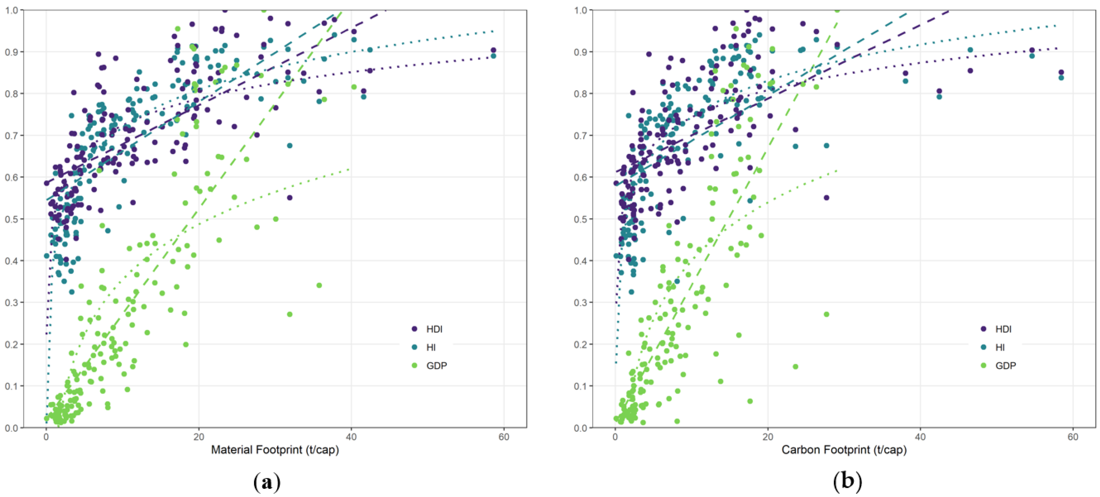
| 1 | HDI vs. MF (1990–2015) | 0.383 ** | 0.138 ** | 0.836 ** | 0.698 | 0.514 ** | 0.012 ** | 0.736 ** | 0.542 | 4000 | |
| 2 | HDI vs. MF | 06–15 avg (Figure 1) | 0.420 ** | 0.130 ** | 0.853 ** | 0.727 | 0.545 ** | 0.012 ** | 0.759 ** | 0.577 | 166 |
| 3 | HI vs. MF | 0.512 ** | 0.092 ** | 0.724 ** | 0.524 | 0.586 ** | 0.009 ** | 0.711 ** | 0.505 | 154 | |
| 4 | GDP/cap vs. MF | −0.126 ** | 0.226 ** | 0.727 ** | 0.529 | 0.003 | 0.028 ** | 0.833 ** | 0.694 | 164 | |
| 5 | HDI vs. CF (1990–2015) | 0.401 ** | 0.130 ** | 0.768 ** | 0.590 | 0.569 ** | 0.008 ** | 0.532 ** | 0.283 | 4002 | |
| 6 | HDI vs. CF | 06–15 avg (Figure 1) | 0.457 ** | 0.124 ** | 0.800 ** | 0.640 | 0.579 ** | 0.011 ** | 0.635 ** | 0.403 | 166 |
| 7 | HI vs. CF | 0.527 ** | 0.094 ** | 0.701 ** | 0.492 | 0.612 ** | 0.009 ** | 0.608 ** | 0.369 | 154 | |
| 8 | GDP/cap vs. CF | −0.116 ** | 0.246 ** | 0.753 ** | 0.567 | 0.001 | 0.035 ** | 0.860 ** | 0.738 | 164 | |
© 2020 by the authors. Licensee MDPI, Basel, Switzerland. This article is an open access article distributed under the terms and conditions of the Creative Commons Attribution (CC BY) license (http://creativecommons.org/licenses/by/4.0/).
Share and Cite
Cibulka, S.; Giljum, S. Towards a Comprehensive Framework of the Relationships between Resource Footprints, Quality of Life, and Economic Development. Sustainability 2020, 12, 4734. https://doi.org/10.3390/su12114734
Cibulka S, Giljum S. Towards a Comprehensive Framework of the Relationships between Resource Footprints, Quality of Life, and Economic Development. Sustainability. 2020; 12(11):4734. https://doi.org/10.3390/su12114734
Chicago/Turabian StyleCibulka, Stefan, and Stefan Giljum. 2020. "Towards a Comprehensive Framework of the Relationships between Resource Footprints, Quality of Life, and Economic Development" Sustainability 12, no. 11: 4734. https://doi.org/10.3390/su12114734
APA StyleCibulka, S., & Giljum, S. (2020). Towards a Comprehensive Framework of the Relationships between Resource Footprints, Quality of Life, and Economic Development. Sustainability, 12(11), 4734. https://doi.org/10.3390/su12114734