Assessment of Exposure to Electric Vehicle Inductive Power Transfer Systems: Experimental Measurements and Numerical Dosimetry

Abstract

High-power inductive power transfer (IPT) systems for charging light and heavy electric vehicles pose safety concerns if they are installed in uncontrolled environments. Within the framework of the European Project EMPIR-16ENG08 MICEV, a wide experimental and numerical study was conducted to assess the exposure of the general public to IPT stray magnetic fields for two different exposure scenarios: (1) for an IPT model system derived from the SAE J2954 standard operating at 85 kHz for a light electric vehicle coupled with the model of a realistic car-body model; and (2) for an IPT model system with a maximum rated power of 50 kW at 27.8 kHz for a real minibus that was reproduced with some simplifications in two different 3D finite element method (FEM) simulation tools (Opera 3D and CST software). An ad hoc measurement survey was carried out at the minibus charging station to validate the simulations of the real bus station for both aligned and misaligned IPT coils. Based on this preliminary study, a safety factor was chosen to ensure a conservative dosimetric analysis with respect to the model approximations. As highlighted in this study, the vehicle-body serves as an efficient screen to reduce the magnetic field by at least three orders of magnitude close to the coils. By applying FEM, computed spatial distribution to the Sim4Life software, the exposure of three Virtual Population human anatomical phantoms (one adult, one child, and a newborn) was assessed. The three phantoms were placed in different postures and locations for both exposure scenarios. The basic restriction limits, established by the current guidelines, were never exceeded within the vehicles; however, the basic restrictions were exceeded when an adult crouched outside the minibus, i.e., near the coils, or when a newborn was placed in the same location. Borderline values were observed in the light car. In the case of the bus, limits coming from the Institute of Electrical and Electronics Engineers (IEEE) guidelines are never exceeded, while basic restrictions coming from the International Commission on Non-Ionizing Radiation Protection (ICNIRP) guidelines are exceeded up to 12% for an adult and up to 38% for a newborn. This paper presents novel dosimetric data generated in an IPT system for heavy vehicles and confirms some of the literature data on light vehicles.

1. Introduction

Inductive charging based on the resonant coupling is a promising charging technology that will be deployed by manufacturers of electric vehicles (EVs) in the near future. Traditional inductive power transfer (IPT) was developed by Nikola Tesla in 1914 [1], and since then, many developers have improved the technology to avoid undesirable strong stray magnetic fields and increase the total efficiency of the power transfer [2,3]. In this context, IPT systems have been tested in recent decades in a wide variety of applications with power transfer ranging from a few milliwatts to several kilowatts. Specifically, from the point of view of applying the technology for EV charging purposes, there are two different approaches: (1) the secondary coil harvests energy as it moves above the primary coil (dynamic inductive power transfer—DIPT); (2) both primary and secondary coils are fixed, facing each other (static inductive power transfer—IPT). This paper deals with the latter approach.

The IPT technology offers many advantages, including the possibility of charging in parking lots or at traffic lights without having to leave the vehicle, smaller batteries, high autonomy, high-efficiency power transmission leading to a reduction in CO₂ emissions, and less oil consumption. The EV global wireless charging market is predicted to record a Compound Average Growth Rate (CAGR) of up to 45% by 2023 [4]. However, an effective EV charging infrastructure must meet specific requirements in terms of a large air gap, high power, and efficiency [5]. Furthermore, some issues regarding storage lifetime, passenger vehicles, required city infrastructures, as well as the energy and environmental impact, must be considered [6].

IPT systems require voltages from 400 V up to 1 kV to supply the charging units with high currents involving tens of amperes. An alternating/direct current (AC/DC) conversion is carried out downstream of the connection point to the electricity grid, while a second DC/AC conversion is performed at the point of resonant inductive power transmission. Finally, an AC/DC conversion takes place in the vehicle to recharge the batteries. The power transmitted from the individual inductive charging unit can be up to 40 kW for a car and up to 180 kW for a truck. The power transfer, depending upon the vehicle type, takes place in the 20–150 kHz frequency band.

The high power required to charge the EV increases concern about the safety of people near the system during the battery charging with respect to the electromagnetic field exposure [7]. Since IPT technology for charging EV is relatively new, standardization activities related to the design of IPT systems for charging EV, as well as established methods to perform experimental measurements for the assessment of human exposure, are still evolving. Currently, the Society of Automotive Engineers (SAE International), formerly the US Society of Automotive Engineers, issued the only existing standard (SAE J2954, [8]), which addresses the issues of the assessment of the transmission efficiency and of human exposure providing general guidelines and suggesting the use of detailed anatomical body models for dosimetry assessment. This standard is limited to light vehicles (≤22 kW) and to static inductive charging at a specific frequency (85 kHz), and its primary aim is to achieve the interoperability between the production of standardized IPT systems for light cars and their testing. SAE J2954 does not cover the accuracy and traceability issues of electric and magnetic measurements. Moreover, the International Electrotechnical Committee (IEC) has established different working groups dealing with the design and the measurement methods of IPT systems. No established measurement method suitable for IPT systems has been standardized yet. If the maximum incident magnetic field generated by the IPT systems is compared to the reference level limits [9,10,11] without considering the effect of the strong inhomogeneity of the field close to the source, a reduction of the maximum allowed power transfer could be required. Therefore, the working group IEC TC106 PT63184 is developing new methods for the measurements of electromagnetic fields (EMF) generated by near-field IPT systems and for the assessment of human exposure in the frequency range 1 kHz–30 MHz.

The existing practices tend to avoid evaluation of compliance with basic restrictions (BR) and are mainly based on testing to verify the respect of the maximum amplitude value of the incident field limits (Reference Levels), which might be over-conservative and lead to an over-strict limitation in the performance of these devices. Indeed, the current RL-based method does not account for the high spatial variability of the MF generated by IPT systems. So, a new BR based compliance testing method has been developed. Specifically, this involves measuring both the magnetic field amplitude and its gradient and relating these measurements to the induced fields in the human body through suitable coupling transformation functions [12]. This new method has been adopted within the IEC TC106 PT63184 draft standard, which will be available at the end of 2021.

Some studies have already analyzed in detail the exposure from static IPT systems. In the paper by Park (2018) [13], the exposure of a human body in proximity to an 85 kHz IPT system was investigated by laboratory experiments and simulations for various transmitting powers and compared to the limits of the 1998 and 2010 ICNIRP guidelines. The maximum allowable transmitting powers were found by means of a dosimetric simulation using the TARO human voxel model (developed by the National Institute of Information and Communications Technology) standing in front of the IPT system. A metal plate on the system simulated the vehicle floor pan.

The exposure of a human standing beside the vehicle (7 kW, 85 kHz) was simulated in the study published by Laakso and Hirata [14], where a generic model of the vehicle was used with the consideration of aligned and misaligned transmitting and receiving coils. The induced electric fields in three anatomically based human models were found to be below the ICNIRP basic restriction, although the external magnetic field exceeded the reference level.

A generic car model was also used in the dosimetric analysis reported by Shimamoto et al. [15], presenting a light vehicle operating at 7 kW and 85 kHz. In this work, the in-situ electric field was evaluated for different postures in the human models. In each scenario, it was confirmed that the maximum induced electric field values are lower than the allowable limit prescribed by international guidelines, despite the limits for the external incident magnetic field not being satisfied. The highest electric field values were observed when the human body was placed on the ground with an arm extended toward the coils.

The specific effect of the car-body was investigated by De Santis et al. and Miwa et al. [16,17], based on generic models of the different cars. In [16], two realistic anatomical models (posable human models ‘Duke’ and ‘Fats’ from the IT’IS Foundation Virtual Population) were placed near or inside an electric vehicle made of carbon-fiber composites with the inductive coils operating at 7.7 kW and two different frequencies of 85 kHz and 150 kHz. The ICNIRP basic restrictions were exceeded, for aligned and misaligned coil positions, only in a small area of the driver’s foot. In [17], the effect of different car-body materials (iron, aluminum, and carbon fiber) on the induced electric field was studied, using the Japanese adult male anatomical model “TARO”.

More complex exposure conditions were considered in [18] by Wang et al. where three exposure scenarios of adult and child models (CAD models derived in accordance with Chinese adult body size in the Chinese National Standard GB10000-88) for a 10 kW, 85 kHz IPT system were investigated. The exposure limit (ICNIRP 2010) was generally satisfied with the adult model standing behind the car and sitting in different positions inside the car. The limits were exceeded in small parts of the adult and child models when they were lying behind the car.

The exposure to the magnetic field leakage from parallel wireless power transfer (WPT) systems working with phase difference was analyzed by Wen and Huang [19]. The maximum rated power was 55.5 kW and 3.1 kW to meet the ICNIRP basic restrictions and the reference levels, respectively.

An experimental approach for determining the induced electric field for exposure evaluation of WPT systems by using measured magnetic near-field data was proposed by Chakarothai et al. [20]. Numerical dosimetry of human exposure was performed by a modeling approach based on the impedance method, where the human model is represented by an equivalent electrical network. The measured near field was used as the incident field, to derive the induced electric field strength inside the realistic human models of the Japanese adult male “TARO”.

Finally, studies that propose a methodology for the assessment of the human exposure to pulsed magnetic fields generated by dynamic IPT systems start to be published [21], showing how the comparison with safety standards and guidelines can be efficiently evaluated by means of a time-harmonic formulation.

In this paper, we report the results obtained in the framework of a wide European project [22] that aims to extend the published analysis for the cases of a car and a bus operating on a virtual and on a real charging station, respectively, through measurements and calculations in order to evaluate the exposure of the occupants and bystanders. The aim of the project is to develop high-accuracy measurement systems, calibration facilities, and models to ensure traceability of the magnetic field measurements performed on static and dynamic IPT systems for charging light and heavy EVs. The results of the above-mentioned project reflect in the main novelties of this paper, which can be summarized as below detailed.

First, a dosimetric analysis was performed based on the assessment of stray magnetic field measurements around a realistic IPT charging station. A measurement campaign was performed on a static IPT system developed at the laboratory of the Centro de Investigación de Recursos y Consumos Energéticos (CIRCE Foundation) in Zaragoza, Spain, for the electric charging of a minibus. A numerical model of this specific IPT system has been developed, validated, and used to assess human exposure by means of numerical dosimetry.

Secondly, the dosimetric analysis was performed, overcoming the limitations of using generic models of the vehicle and IPT systems, which do not fully represent the reality. Here, two realistic models of a light vehicle (a Volvo car) and a heavy vehicle (the minibus of the CIRCE charging station) were developed, taking into account the realistic properties of the respective car-bodies. This is the first dosimetric analysis in which exposure of passengers in public vehicles was considered and compared with the exposure from light vehicles.

Finally, advanced high-resolution human anatomical models were used for the numerical dosimetry. These models belong to the Virtual Population [23,24] (ViP, developed by the Foundation for Research on Information Technologies in Society (IT’IS), Switzerland) and represent a wide range of the population in terms of age, size, and weight. Critical exposure scenarios were analyzed by placing the human anatomical models in different postures, either close to the vehicle or inside it. For each exposure configuration, the induced fields were calculated and compared with the current exposure guidelines [9,10,11].

The combination of the above mentioned three aspects makes the contribution reported in this paper original with respect to articles already published in the literature.

2. Materials and Methods

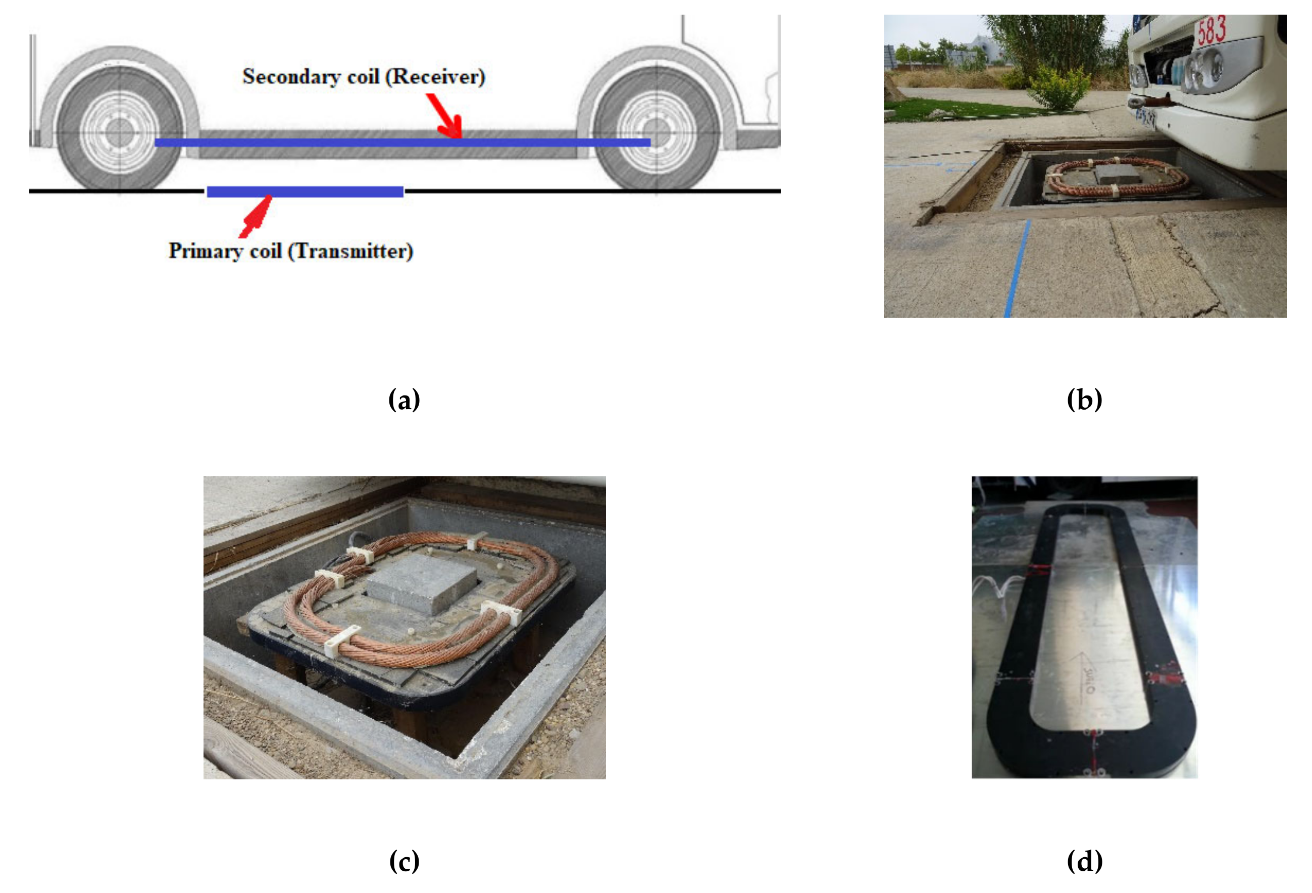
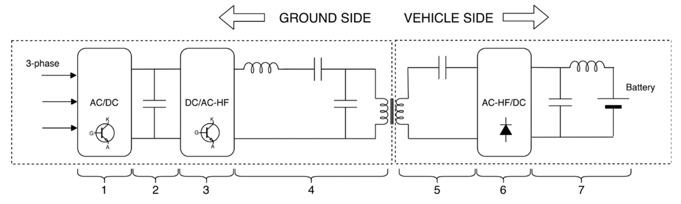
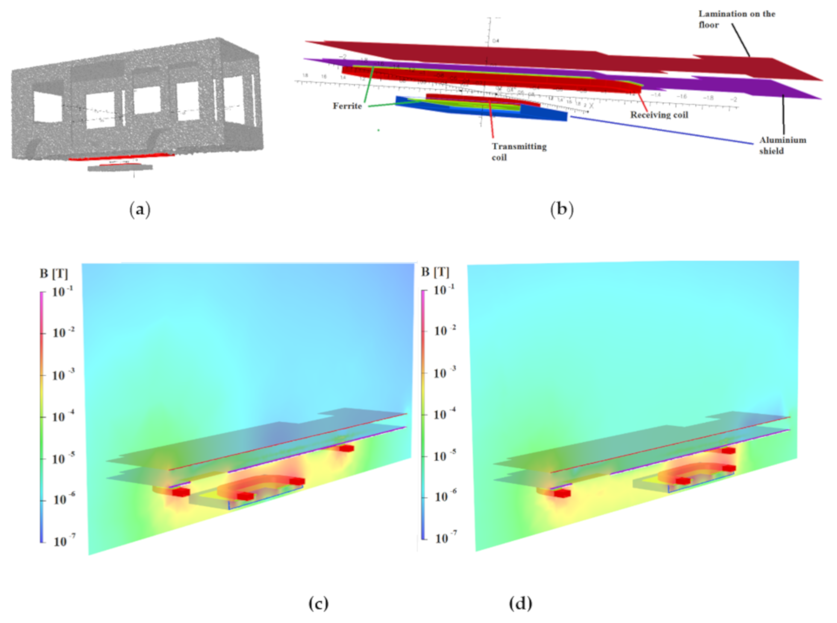
2.1. WPT Systems for the Bus: Tested Charging System

The first part of this study was conducted at the CIRCE EV laboratory on a static heavy-duty IPT system with a rated power of 50 kW and a switching frequency close to 27.8 kHz. The charging station design was patented by CIRCE, and it relies on a Series-Parallel-Series (SPS) scheme allowing for considerable misalignment between primary and secondary coils without significantly compromising the overall efficiency. The ground coil size was 0.8 m × 0.6 m, and the onboard coil was 2.5 m × 0.6 m (Figure 1a). The transmitting coil (TX) was surrounded by an aluminum boxed screen, and a layer of ferrite was placed under the coil. The receiving coil (RX) had a ferrite layer that runs around the profile of the coil, behind it (Figure 1b). An aluminum shield with dimensions similar to those of the bus floor was placed in contact with the ferrite layer. The bus floor was made of steel sheet and was situated 14 cm above the aluminum screen.

The structure of the bus coils maintained a total efficiency of around 85% with a maximum misalignment of ±30% (regarding the primary coil area) and a working air gap of 0.15 m to 0.25 m between the coils. The heavy test vehicle was a Technobus Gulliver U520 ESP/LR electric bus with an inductive fast charging capability of 50 kW. Figure 2 shows the electrical block diagram of the IPT system.

In Figure 2, the first block comprises one insulated gate bipolar transistor-(IGBT)-based AC/DC grid multilevel converter, an internal 700 V DC bus, and one DC/DC buck converter. Block 2 corresponds to a variable DC bus (range 70–500 V). The third block includes a DC to AC high-frequency H-bridge converter that feeds Block 4, the primary Series-Parallel resonant tank. The current observed inside the tank can reach up to 1000 A. On the vehicle side (inside the vehicle), the secondary Series resonant tank can be found in Block 5. After that, an AC high frequency to DC secondary converter (Block 6) filters and converts the AC power captured by the secondary coil to DC to charge the EV batteries (Block 7).

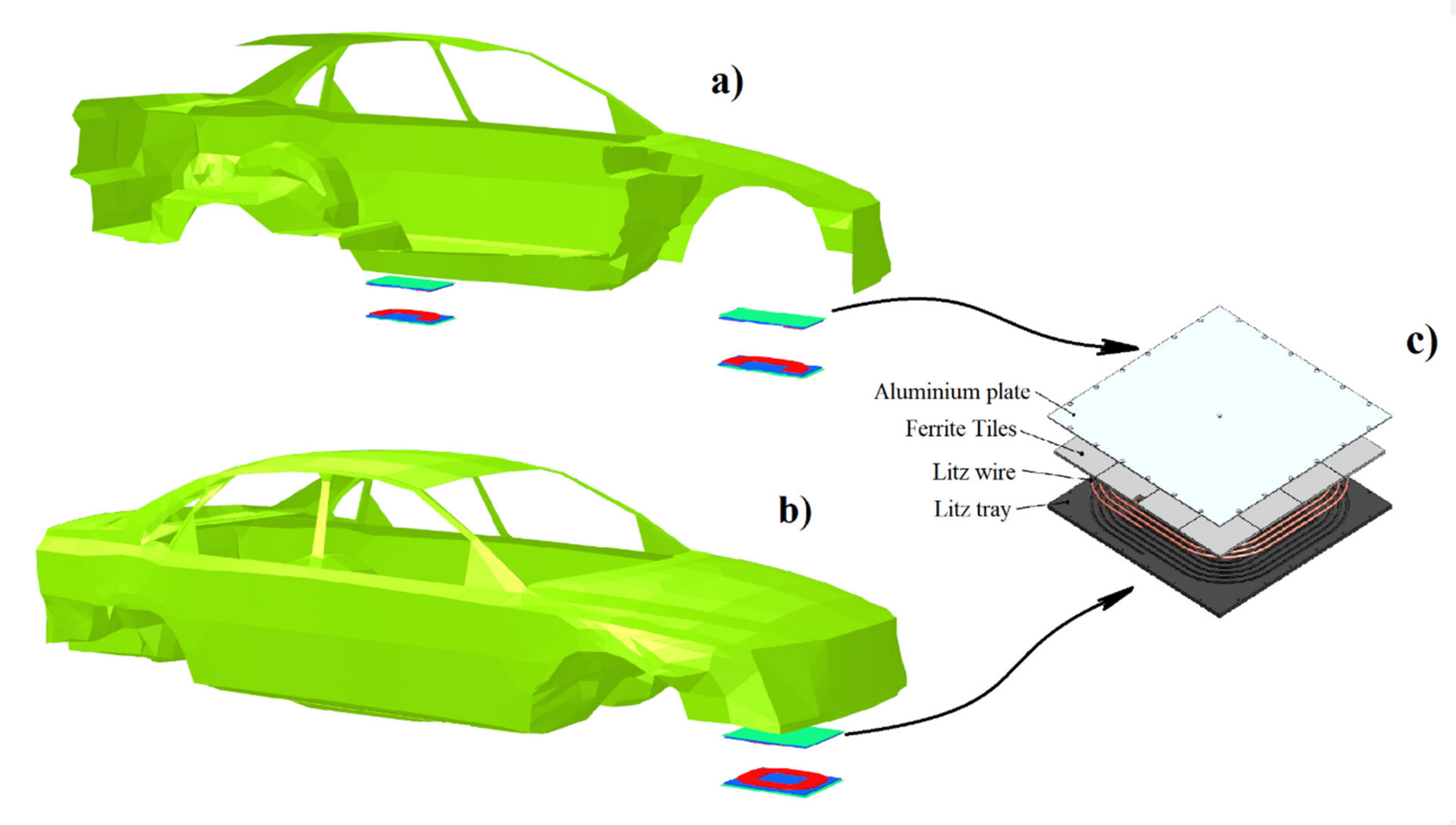
2.2. WPT Systems for the Light Vehicle

In accordance with the SAE standard [8], a class WPT2 system (power up to 7.7 kW) with a Z3 clearance between the ground and the vehicle assembly coil (170<Z3<250 mm) was used for the light vehicle. The structure recommended by the SAE J2954 standard (paragraph F1.2) was adopted for the transmitting and receiving coils, in which the coil was placed in a flat, square structure with a side length of 380 mm and rounded corners (100 mm radius). It consisted of eight turns with a 5 mm diameter Litz wire. The transmitting coil was placed on top of a ferrite plate with a side of 420 mm, at a reciprocal distance of 6 mm. The ferrite plate was 5 mm thick and placed on an equally sized aluminum shield at a reciprocal distance of 5.6 mm.

The receiving coil had the same structure as the transmitting coil, except it was its mirror-image, and the distance between the coil and the ferrite layer was reduced to 1 mm. The current in the two coils was taken as sinusoidal, the current in the receiving coil being the same amplitude as that in the transmitting coil (i.e., 26 A, or 208 A-turns peak value), but the electric current in the receiving coil had a 90° phase lag.

The coils were combined with the car-body of a Volvo S80 sedan, supplied by the Volvo car company. Two receiving coil positions were considered: (1) at the front of the car and (2) at the center of the car. Figure 3a shows the cross-section of the sedan with the two possible positions of the charging system. Figure 3b shows the complete car-body with the charging coils placed at the front of the car. For the centrally positioned system, the distance between the coils was 150 mm, whereas the distance between the coils is 200 mm for the system positioned at the front of the car.

2.3. Measurements Protocol Adopted at the Bus Station

The verification measurements were carried out on the minibus at the CIRCE charging station in Zaragoza, Spain. The experimental verification and the simulation comparisons using this set-up could be considered representative for both light and heavy vehicles. The magnetic flux density measurements were synchronized to the electrical measurements of (coil currents) to correlate the magnitude of the magnetic flux density directly with the amplitude and phase of the currents. The instrumentation and methods are described in the following sub-paragraphs.

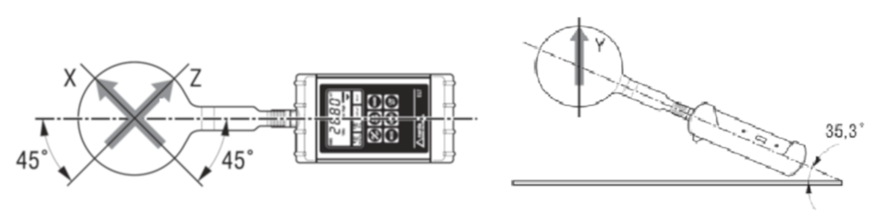
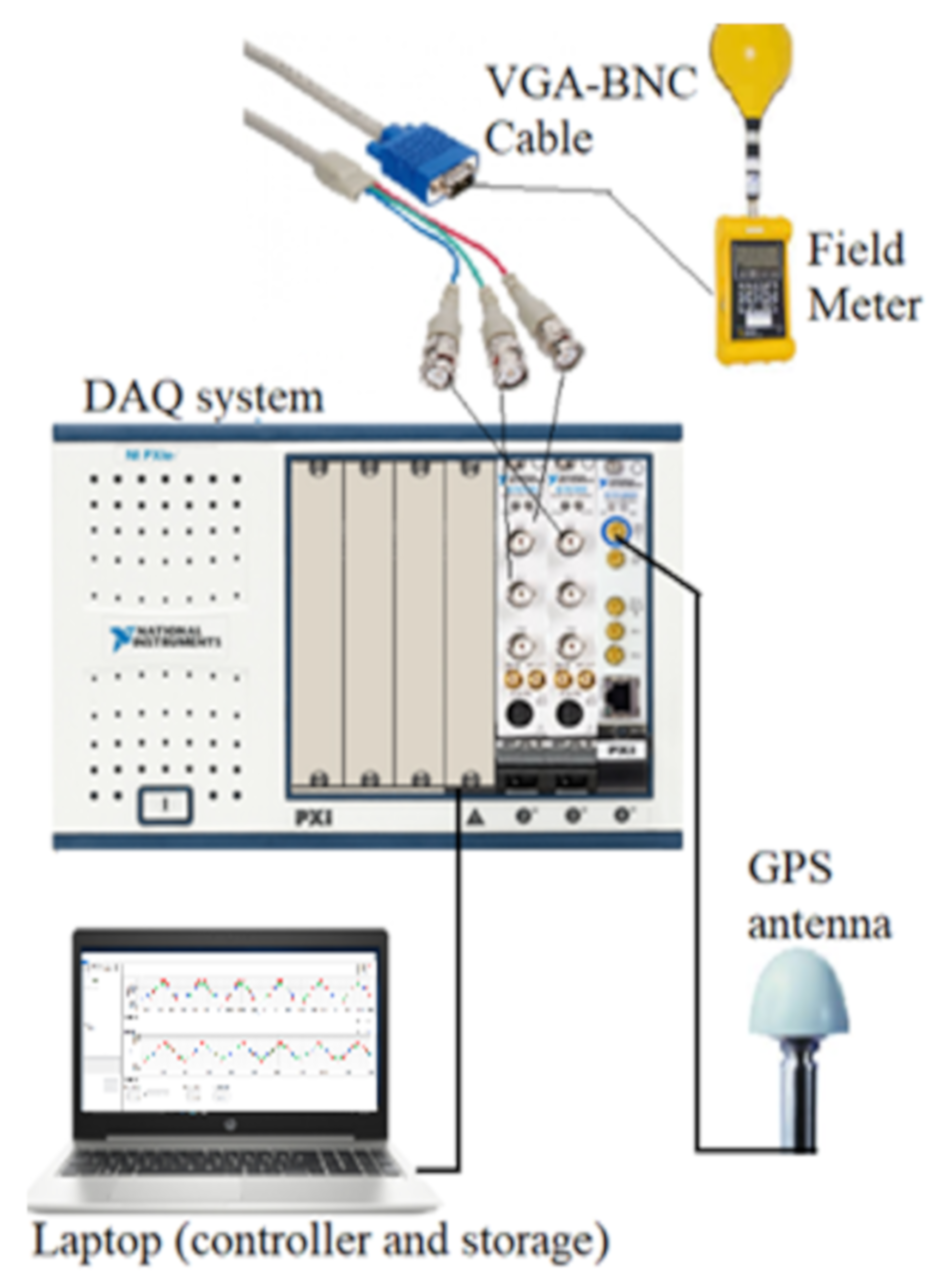
2.3.1. Instrumentation

A Narda ELT-400 magnetic field measuring instrument consisting of three-axis magnetic flux density (B-field) sensing probes and a meter displaying the field amplitude (root mean square, r.m.s. value) was used. These instruments also provide the r.m.s. of the three B-field components (through a serial port), and the analog signals corresponding to the field waveforms (through a video VGA port). This instrument, which complies with EN 62,233 Standards [25], has been chosen for three main features: (a) an adequate frequency band, (b) the presence of the analog output, (c) the availability of probes with concentric coils, which are more reliable for measurements of spatially non-uniform fields [26].

The Narda ELT-400 has two different types of B-field probes with 100 cm² and 3 cm² cross-sectional areas. The coil layout for both probes is illustrated in Figure 4.

Both probes were calibrated in accordance with the on-site measurement conditions at the National Physical Laboratories (NPL) facility (meter with 100 cm² probe) [22], and at the Istituto Nazionale di Ricerca Metrologica (INRiM) facility (meter with 3 cm² probe) [27]. The meter with the 100 cm² probe demonstrated an instrument error <1% for indicated fields greater than 0.4 µT (see Section 2.3.4), while the meter with the 3 cm² probe showed a higher error up to 5%. Thus, the meter with the 100 cm² probe was used in the measurement campaign.

The magnetic field probes were integrated into the Power Measurement Unit (PwMU), which is a complete measurement system for the characterization of charging stations for EVs, developed by the INRiM and described in detail in [28]. It consists of three parts: (1) a grid unit for the ground measurements, (2) a board unit for the measurement on-board, and (3) a magnetic unit for the measurement of the magnetic flux density. The measurements by the three parts are synchronized through cards making use of the Global Positioning System (GPS) signal. The synchronization accuracy is better than 100 ns.

The coil currents were measured using a synchronized data acquisition system based on a National Instrument PCI eXtensions for Instrumentation (PXI) architecture. Since the coil currents reached 1 kA, two precision Rocoil Rogowski coils coupled with a 7000 series three channel integrator (Rocoil Rogowski Coils Limited, Harrogate, North Yorkshire, UK) were used as the sensors for the current measurements, allowing for accurate measurement of the phase angle between current phasors with a resolution better than 0.01 degrees. Both the modulus and phase of the transmitter and receiver currents were measured, the waveforms were recorded, and the r.m.s. values were computed and stored.

The field meter was connected to the data acquisition system (DAQ) by a video BNC cable. The DAQ system was based on two synchronized PXI 5922 oscilloscope card modules, which allows for the acquisition of the magnetic field component waveforms. The programming of the data, including the waveforms, was synchronized to the acquisition time on the GPS board (GPS timestamp). Finally, a module with an MXI (link for PCI-to-PXI) interface connected the system to a laptop that manages the measurement control program and data storage. A schematic of the magnetic measurement system is shown in Figure 5.

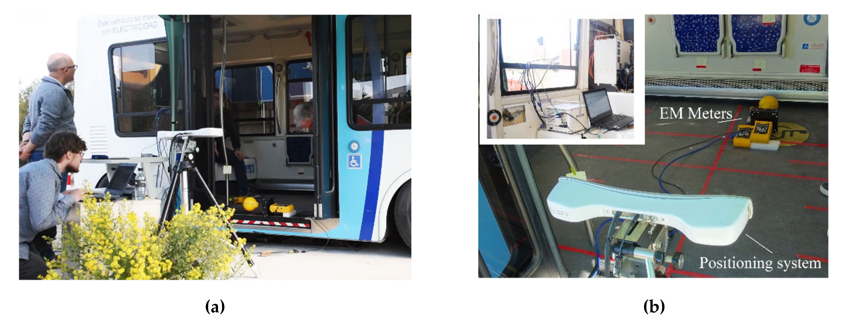
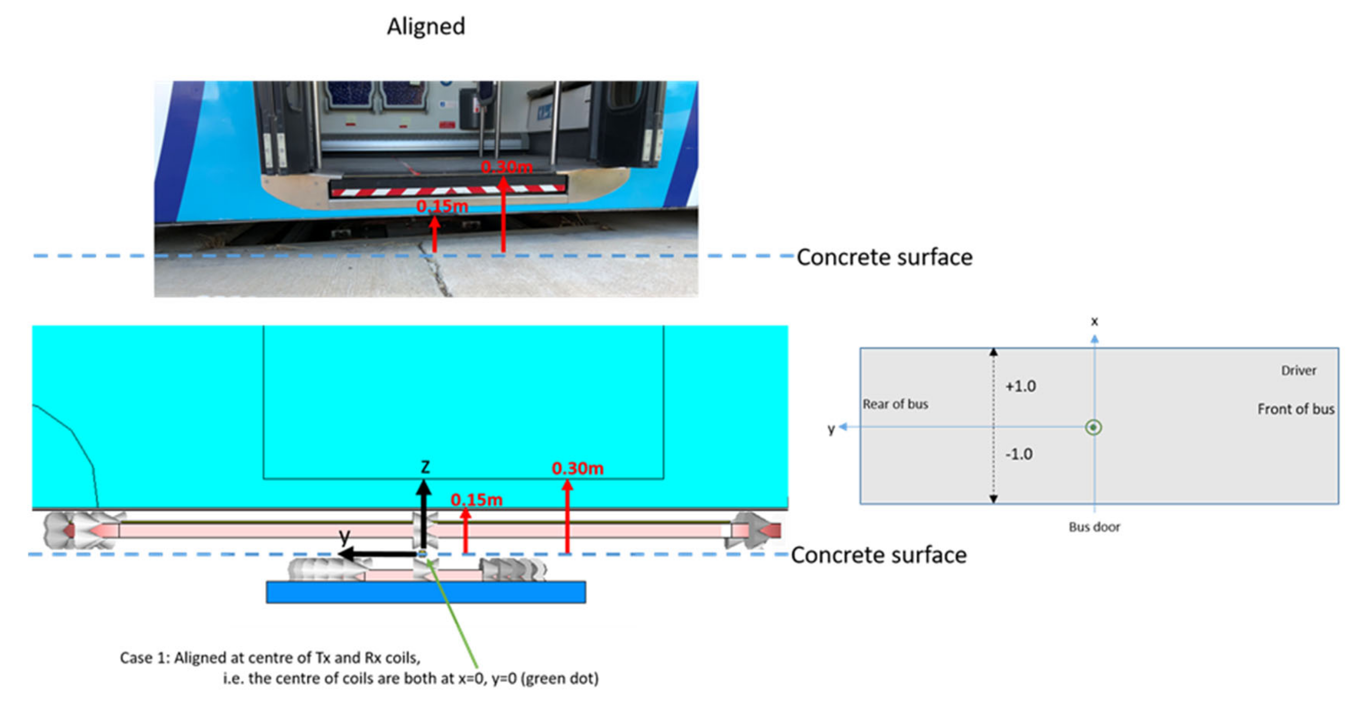
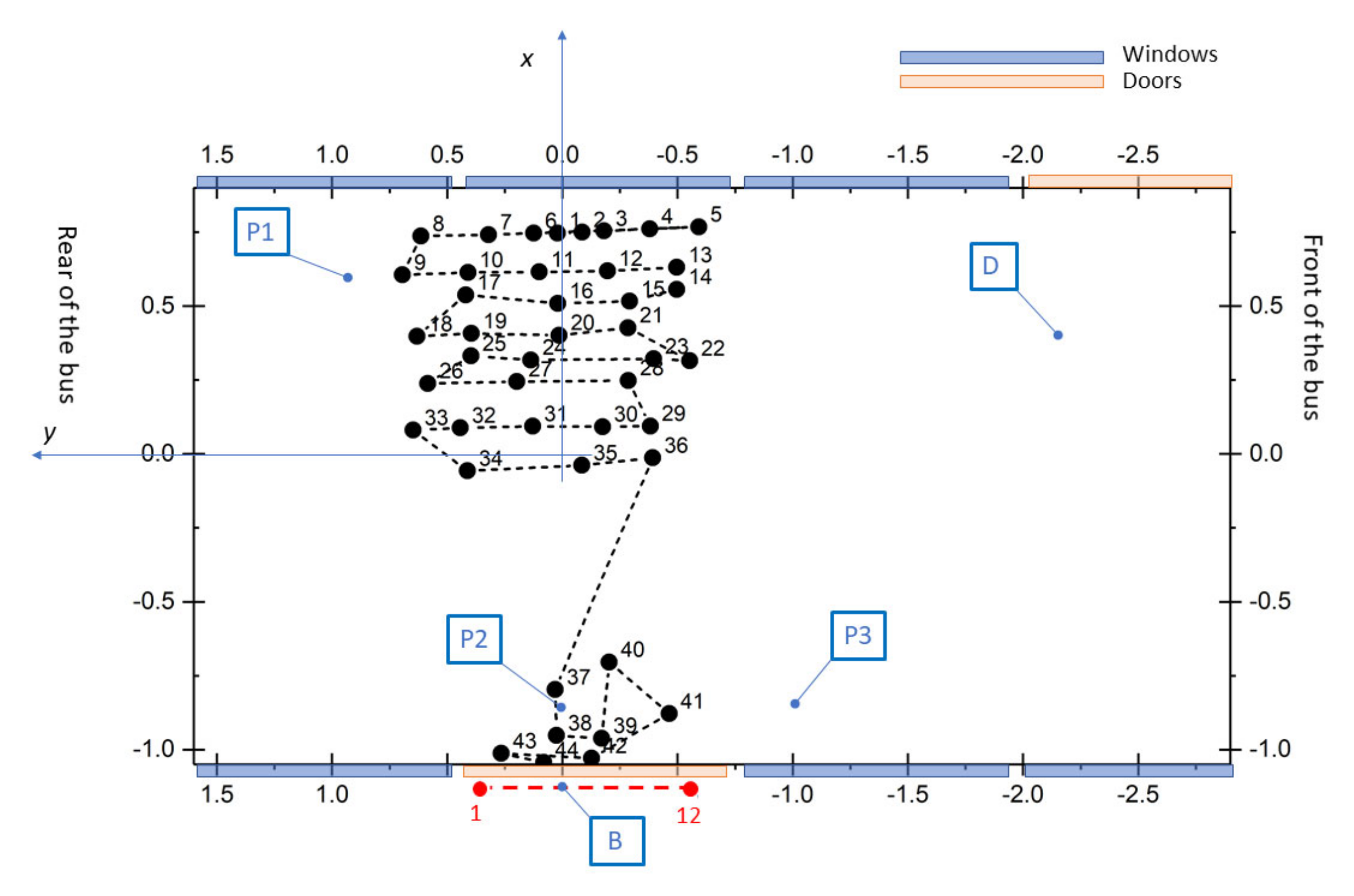
2.3.2. Positioning System

A ‘PST Iris HD’ stereo-vision camera system manufactured by PS-Tech [29] tracked the Narda ELT-400 probe. This system uses pre-set reference points to track the position of an object. The tracking points used for the probe were attached to the probe’s neck and defined the target’s center as the center of the probe-head. The PST Iris used a local coordinate system with its origin set at 1 m in front of the camera in the orientation of the camera. Since the latter needed to be moved around the vehicle to acquire all measurement data points, they were translated and rotated into a global co-ordinate system. This global coordinate system was built using static tracking targets of accurate known positions, allowing for accurate position measurements in the global coordinate system. If the two static targets and the probe-head target were visible, the physical camera could be moved arbitrarily, and the software reading the target locations could calculate the global position by using basic rotational matrices. The expanded uncertainty of the locations measured with the PST Iris system in 2D was estimated to be ±0.64 mm [29]. The software developed at NPL acquired the timestamp, global $\left(x,y,z\right)$ coordinate of the probe and the field measurement for each location, and wrote this data matrix onto a file for processing at a later time. The measurement layout is shown in Figure 6.

2.3.3. Measurement Procedure

A measurement procedure was carried out according to the steps listed below and repeated for each measurement point:

• Place the probe at one measurement point;
• Adjust the software setting of the measurement time instant for the acquisition and measurement systems, based on the synchronization cards;
• Switch on the charging station power supply. The system starts running in a few seconds;
• Upon the automatic start of the measurement, the measured values were recorded by the acquisition software, including the coil currents and the r.m.s. values of the resulting magnetic induction at the measurement point.

Measurements were carried out under two operating conditions: aligned and misaligned TX and RX coils. A schematic of the centered and misaligned conditions, together with the adopted reference coordinate system is shown in Figure 7. In both cases, the reference system was always located on the TX coil to ease the comparison of the data.

Three measurement sessions (S.1, S.2, S.3) were recorded, as shown in

Table 1. Data of the three measurement sessions: TX and RX coil positions, currents (amplitude and phase shift), and the measurement regions for each session. The ratio between TX and RX current amplitude between the different sessions depends on the system configuration and the setting of the supply parameter control.

Session	TX, RX Coil Position	TX Current (A)		RX Current (A)		Phase Shift (deg)		Measurement Region
		Avg.	Std. Dev.	Avg.	Std. Dev.	Avg.	Std. Dev.
S.1	Aligned	427	8	108	23	89	1.5	Inside bus at floor level
S.2	Aligned	485	3	81	0.5	82	0.3	In three passenger positions (P1, P2, P3), in bystander position (B) and in driver position (D)
S.3	Misaligned (0.843 m along the y-axis)	711	78	83	0.4	76	0.6	Along three lines at different heights along the bus entrance

. For the first two sessions, the TX and RX coils were aligned, then the bus (and, therefore, the receiving coil) were transferred by a distance equal to 0.843 m along the y direction for the third session. The average values of the TX and RX current amplitudes, the phase shift, and the standard deviation of the measurement datasets are reported in Table 1.

In session S.1, a series of 44 measurement points were characterized inside the bus at the floor level. The point sequence is shown in Figure 8 as a black dashed line. The measurement ID was also reported close to the symbols. In session S.2, the spot measurements were performed within the bus for key positions, corresponding to three passengers (P1, P2, and P3), a bystander, and (B) the driver (D) (see Figure 9). For each position, four heights were considered: ankle level, knee level, trunk level, and head level. The corresponding heights are shown in

Table 2. Height from the ground road level of the measurement points.

Position	Outside the Bus	Inside the Bus
Ankle	Z = 0.1 m	Z = 0.28 m
knee	Z = 0.5 m	Z = 0.7 m
trunk	Z = 1.4 m	Z = 1.6 m
head	Z = 1.7 m	Z = 1.9 m

. Finally, for the misaligned TX and RX coils in session S.3, measurements were made along a line close to the bus entrance door, at two different heights from the ground floor (0.10 m and 0.21 m). The measurement sequence is shown in Figure 8.

2.3.4. Uncertainty Analysis of On-Site Measurements

Uncertainty assessment relies on well-known international guidelines and methods [30,31]. The methods applied in this paper were based on splitting the total uncertainty into several components that are uncorrelated or with limited interdependency, determining the uncertainty from assumed statistical models, and calculating the total uncertainty as a root-sum-square (RSS) value. In accordance with the guidelines, the effective degrees of freedom apply to statistically derived uncertainties for which the sample sizes were used to determine the coverage factor—they were assumed to be infinite for all Type B evaluations. Throughout the analysis used here, all uncertainty components were assessed using Type B evaluation; hence, the degrees of freedom were taken to be infinite. Each uncertainty source listed below is shown in the format: “uncertainty source: description of each uncertainty component”.

• tolerance in dB: the tolerance of each component, expressed in dB in terms of its influence on the quantity of interest;
• probability distribution (distr): the variation in the probability of the true value lying at any particular offset from the measured result. R-(log)rectangular distribution, N-(log)normal distribution;
• divisor (div): either 2 for a normal distribution or $\sqrt{3}$ (1.7321). A divisor of $\sqrt{3}$ relates the standard uncertainty of a rectangular distribution to a normal distribution;
• sensitivity coefficient ($c_i$): the sensitivity coefficient of each uncertainty component that translates the unit of the tolerance to the unit for which the uncertainty is determined. Since all tolerances are already expressed in dB relative to the quantity of interest in this work, the sensitivity coefficient is unity for all contributing components and set to zero for irrelevant components;
• standard uncertainty in dB (std unc): the contribution of the uncertainty component to the combined standard uncertainty.

The expanded uncertainties (k = 2 for 95% coverage factor) for the calibration of the ELT-400 under laboratory conditions were:

• ±0.55% at instrument indications of 0.8 µT and above;
• ±1.0% at instrument indications in the range of 0.2–0.8 µT;
• ±5.0% at instrument indications below 0.2 µT.

The spatial uncertainty accounting for the averaging effect of the B-field probe was estimated from simulations using the CST Software and the computed B-field spatial distribution generated by the CIRCE charging station. Specifically, a cubical B-field probe with a 7 cm side and a 12 cm diagonal was used, and the B-field was sampled at 343 equally-spaced points by means of interpolation. For each of these points, the average of the B-field for the cubical probe and the B-field value at the center of the probe were calculated. The cubical probe dimensions ensured a good “fit” inside the spherical probe (ELT-400 probe) used in the field measurements; thus accounting for most of the statistical data (mean and standard deviation). The mean relative uncertainty for the B-field (labeled “Spatial uncertainty accounting for probe volume” in

Table 3. Uncertainty budget for magnetic field measurements where the 3D Tracker was used.

Source of Uncertainty	Value	Probability	Divisor	c1	u1
	%	Distribution			%
Calibration of ELT-400	0.55	Normal	2	1	0.275
3D tracker positional accuracy (automated)	0.23	Rectangular	1.7321	1	0.133
Spatial uncertainty accounting for probe volume	0.30	Normal	2	1	0.150
Reproducibility	0.10	Normal	2	1	0.050
Combined uncertainty for 3D tracked measurements		Normal			0.344
Expanded uncertainty for 3D tracked measurements		Normal	k = 2		0.688

and

Table 4. Uncertainty budget for magnetic field measurements performed manually.

Source of Uncertainty	Value	Probability	Divisor	c1	u1
	%	Distribution			%
Calibration of ELT-400	0.55	Normal	2	1	0.275
Manual positional accuracy	2.80	Rectangular	1.7321	1	1.617
Spatial uncertainty accounting for probe volume	0.30	Normal	2	1	0.150
Reproducibility	0.10	Normal	2	1	0.050
Combined uncertainty for 3D tracked measurements		Normal			1.647
Expanded uncertainty for 3D tracked measurements		Normal	k = 2		3.295

) was calculated by comparing the mean B-field for the cubical probe and the B-field at the center point of the probe.

The positional accuracy for 3D tracked measurements was estimated as detailed in Section III of [29]. An expanded uncertainty of ±0.688% was found for 3D tracked measurements (Table 3). In Table 4, the manual positional accuracy was also estimated with the following simplifying assumption. As the measurements performed in CIRCE were spaced at 10 cm (equal to the NPL probe diameter) during the 2D scans, it was assumed that the positional uncertainty was ±1 cm. From the raw data, the slope of the B curve was considered, and the steepest gradient was used to determine the worst- case corresponding to a positional uncertainty of ±1 cm. This process resulted in a relative uncertainty equal to 2.80%. An expanded uncertainty of ±3.3% was found for manual measurements of the magnetic field.

2.4. Numerical Simulations

2.4.1. Numerical Models of the IPT Systems

The charging system of the light EV was described in Section 2.2 The magnetic field distribution was assessed when the IPT system was placed at the front position and in the central position under the car. Figure 9 shows the positions selected to perform the exposure assessment in human anatomical models when the IPT system was placed under the light EV (car) in either the frontal or the central position (the coils are alternately activated). The exposure was analyzed with and without the EV to evaluate the impact of the car-body on the magnetic field distribution.

The car model is derived from a real car-body (see Figure 3) and was discretized with the Opera 3D software, Dassault Systèmes [32], with 4.72 million nodes, 7.75 million edges, and 6.07 million tetrahedral elements. For validation, a similar model was created with the CST software, Dassault Systèmes [33]. Using a Dell Server PowerEdge R740, with a double processor Intel Xeon Gold 6130, having a total of 32 cores and 256 GB RAM (300 GB SAS), the solution of the FEM car problem providing the magnetic field distribution around and inside the car takes about 16 h (CPU time). The following physical properties were assigned to the materials. (i) car-body (carbon-steel alloy): relative magnetic permeability μ_r = 300, electrical conductivity

σ = 2 MS/m, (ii) ferrite: relative magnetic permeability μ_r = 2000 and negligible electrical conductivity, (iii): aluminum: relative magnetic permeability μ_r = 1, electric conductivity σ = 33.5 MS/m. The simulations were performed at the 85 kHz frequency with the assumption of linear behavior for all materials.

Figure 10 shows the distribution of magnetic induction in a median section of the car for the central charging pad and the charging pad at the front of the car. In both cases, the car-body acted as an efficient screen against the magnetic flux density. The magnetic induction values drop suddenly by three orders of magnitude crossing the edge of the car-body, ranging in value from 0.1 mT close to the charging pad to values near the ambient noise or <10 nT inside the car-body. Higher values inside the EV (~100 nT) were found only in correspondence with the glass surfaces, which obviously suffer from a slightly decreased shielding effect.

The effect of the car door (opened/closed) is shown in Figure 11 for the case of the central IPT. The map of the B-field amplitude is shown at the height z = 0.4 m. The B-field amplitude outside the EV is not affected very much. However, when the door is open, the B-field leaks into the car.

An equivalent model of the bus used at the CIRCE charging station, as described in Section 2.1, was built. A model view showing the bus shape and some of the volume mesh element is presented in Figure 12a. The model includes the main structures that are significant from the viewpoint of the magnetic field (see Figure 12b), namely the ferrite placed close to the coil (μ_r = 2000, σ ~ 0), the metal sheet placed at the base of the floor (μ_r = 300, σ = 2 MS/m), and the aluminum sheet placed above the receiving coil (μ_r = 1, σ = 33.5 MS/m). The transmissions, the joints, and the electrical engine were the only parts disregarded in the models as their effects on the stray magnetic fields were assumed to be negligible. The CIRCE bus-body was made of fiberglass so that its effect was negligible from an electromagnetic point of view. This model was used for the comparison between simulated and measured values. The exposure assessment through the dosimetric analysis was carried out also for the carbon-steel alloy bus-body having the same properties used for the light vehicle (Section 3).

The mini-bus model was discretized with the Opera 3D software with 11.16 million nodes, 23.92 million edges, and 19.06 million tetrahedral elements. The FEM bus problem with fiberglass bus-body was computed in about 10.5 h (CPU time), while about 16 h were needed in the case of a metallic bus-body. Linear material behavior was assumed. The magnetic field distribution was assessed with the receiver coil placed under the bus in the central position and when the coils were being misaligned along the y-axis by 0.843 cm.

Figure 12c,d illustrate the effect of attenuation of the magnetic induction values created by the aluminum screen and the bus floor, for aligned and misaligned coils, respectively. The reported results refer to the fiberglass bus-body. The attenuation effect was less evident than in the case of the light vehicle shown above in Figure 10.

2.4.2. Procedure for the Validation of the Numerical Model of the IPT Systems through On-Site Measurements

The numerical models used for computing the B-field inside and around the IPT systems were validated by comparison with the on-site measurements obtained at the CIRCE charging station. While the measurement of B-field emissions to evaluate the exposure only required a correlation with the power transferred (exposure under a given operating condition), a synchronized acquisition of the current waveforms in the transmitting (TX) and receiving (RX) coils (amplitude and phase shift) was necessary to compare the measurements with the simulations. The measurement protocol described in Section 2.3 was applied.

For each on-site test session, every measurement point was in principle associated with a different pair of current values in the TX and RX coils. The numerical simulations were performed using a unitary current amplitude for the TX or the RX coils. When the TX coil is considered, we obtained the real and imaginary parts of the B-field per unit-current (units are tesla per ampere) for each computational point (b_TX,real(x,y,z) and b_TX,imag(x,y,z)), corresponding to a unitary current flowing in the coil. Similarly, when the RX coil is considered, we obtained: b_RX,real(x,y,z) and b_RX,imag(x,y,z). By taking advantage of the system linearity, the real and imaginary parts of the B-field (B_real(x,y,z) and B_imag(x,y,z)) at any point for any given I_TX and I_RX currents in the TX and RX coils with phase shift α, were then obtained as:

$$\begin{gathered} B_{real}\left(x,y,z\right)=b_{TX,real}\left(x,y,z\right)I_{TX}+b_{RX,real}\left(x,y,z\right)I_{RX}\cos \left(\alpha \right)-b_{RX,imag}\left(x,y,z\right)I_{RX}\sin \left(\alpha \right) \\ {B}_{imag}\left(x,y,z\right)=b_{TX,imag}\left(x,y,z\right)I_{TX }+b_{RX,real}\left(x,y,z\right)I_{RX}\sin \left(\alpha \right)+b_{RX,imag}\left(x,y,z\right)I_{RX}\cos \left(\alpha \right) \end{gathered}$$

(1)

2.4.3. Simulation Protocol for Numerical Dosimetry

The advanced high-resolution anatomical ViP models Charlie (the newborn), Thelonious (body mass index BMI = 13.8 kg/m²), and Duke (BMI = 22.4 kg/m²) were used to perform the numerical simulations. Tissue dielectric properties were assigned according to the IT’IS Foundation Database [34,35] at 27.8 kHz and 85 kHz, respectively. The conductivity of the skin tissue was 0.1 S/m to account for the dermis.

The human anatomical phantoms were placed near and inside the EVs and at the closest locations with respect to the IPT systems. The exposure assessment was performed when the human models were placed in both a standing posture around the EV and in other postures (e.g., crouching on the knees, sitting in and outside the car, lying with an arm stretched towards the IPT system).

Table 5. The most relevant exposure scenarios were analyzed to assess exposure to the IPT system for charging a light EV. The table refers to the positions of the IPT systems and the possible locations outside and inside the EV, as shown in Figure 9.

IPT System Position	ViP Model Position	Posture
Central/Front	B2/B1	Duke standing
Central/Front	B2/B1	Duke crouching on knees
Front	B1	Duke lying with arm stretched
Central/Front	B2/B1	Thelonious sitting
Central	inside the car	Charlie (P2), Duke (DR) and Thelonious (P3) sitting

and

Table 6. The most relevant exposure scenarios were analyzed to assess exposure to the IPT system for charging a bus. In this case, the IPT system was always placed under the bus in the central position.

IPT System Position	ViP Model Position	Posture
Central	outside/front of the door	Duke standing
Central	outside/front of the door	Charlie sitting
Central	outside/front of the door	Duke crouching
Central	outside/front of the door	Thelonious sitting
Central	inside/front of the door	Duke sitting
Central	inside/front of the door	Charlie sitting

summarize the most significant exposure scenarios analyzed in this study to assess the exposure of the ViP phantoms to the IPT systems used for charging the light EV and the bus, respectively.

Two numerical solvers were used to perform the numerical dosimetric analysis. First, the solver Opera 3D (version 18R2) was used to generate the magnetic field distributions of the two IPT systems for each exposure configuration. Since the wavelength was much larger than the exposed object at frequencies <100 kHz, a quasi-static approximation was valid, and the electric and magnetic field exposure could be studied independently. Secondly, the magnetic field distributions generated through the simulation software Opera 3D were then used as magnetic field sources in the magneto-quasi-static (MQS) solver of the simulation platform Sim4Life version 5.0 (ZurichMedTech, Switzerland) [36] to assess the exposure of the ViP phantoms.

2.4.4. Analyzed Metrics

The exposure was assessed with respect to the fields induced in the human body. Specifically, the induced electric field was assessed according to the ICNIRP 2010 [10] and IEEE 2005 [11] guidelines, by taking the peak of the electric field averaged over a 2 mm-side cube and along a 5 mm-line segment, respectively, in each specific tissue and organ. The induced current density was assessed with respect to ICNIRP 1998 [9], by comparing the basic restriction limits to the peak of the induced current density averaged over a 1-cm² disc in the central nervous system tissues.

Table 7. Basic restriction limits for the induced electric fields and current density defined in the ICNIRP and IEEE guidelines.

Guideline	Metric	f = 27.8 kHz	f = 85 kHz	Averaging Method
ICNIRP 2010	Electric field (V/m)	3.75	11.47	2 mm side cube
ICNIRP 1998	Current density (mA/m2)	55	170	1 cm2 disc
IEEE 2005	Electric field (V/m)	5.81	17.76	5 mm line segment

summarizes the basic restriction limits for the induced electric field and current density at 27.8 kHz and 85 kHz. The recently published 2020 ICNIRP Guidelines for Limiting Exposure to Electromagnetic Fields [37] had no impact on this study as it applies to the frequency range 100 kHz–300 GHz. Only the radiofrequency electromagnetic fields (RF EMF) of the ICNIRP 1998 guidelines and the 100 kHz–10 MHz part of the ICNIRP (2010) low-frequency guidelines were updated.

3. Results

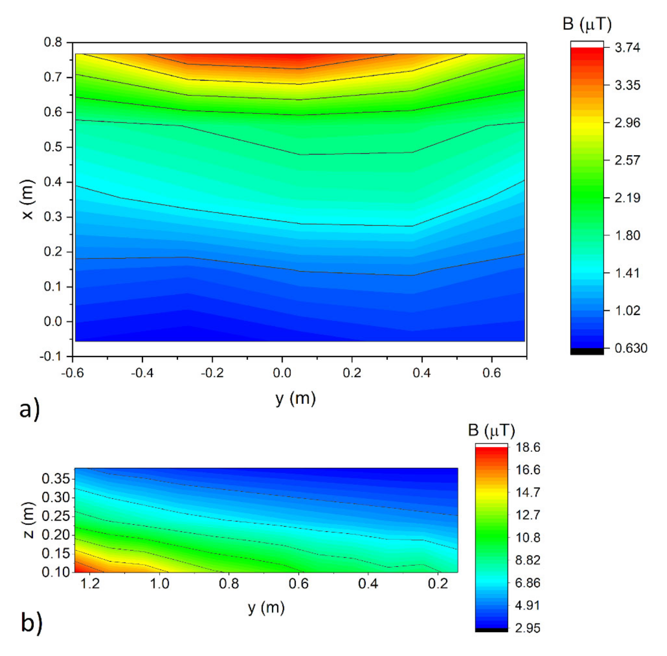
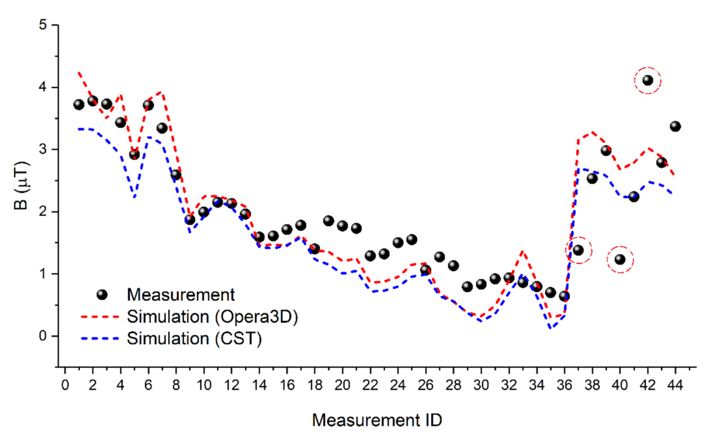
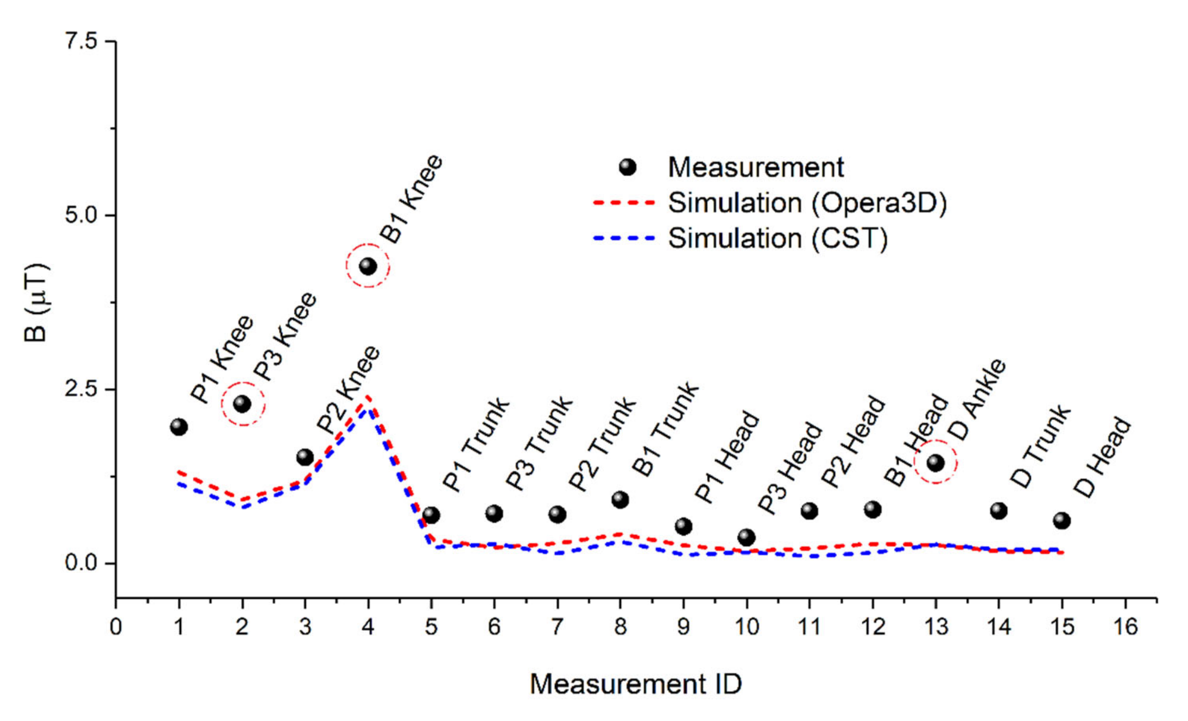
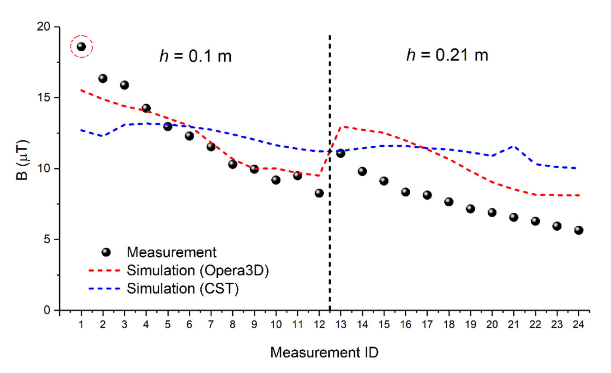
3.1. Comparison between Experiments and Simulations

The B-field measured within the bus had an intensely non-uniform spatial distribution due to the source configuration and the presence of metallic objects, as shown in the plot of the measured B-field amplitude at the floor level for session S.1 (Figure 13a) and from the vertical plot of the B-field amplitude in correspondence with the bus entrance for session S.3 (Figure 13b). The coordinates (x, y, z) here reported corresponding to the reference system introduced in Figure 7 and Figure 8. The highest field intensity was always found near the lateral sides, where the effect of the shield placed between the coils and the bus floor vanished.

The results of the comparison between measured and simulated values using Opera3D and CST are shown in Figure 14, Figure 15 and Figure 16. Discrepancies between results obtained with Opera3D software (B_Opera), CST software (B_CST), and the measured values (B_meas) were calculated and normalized according to the Equation (2):

$$\mathsf{\epsilon } =\left|B_1-B_2\right|/B_{avg}$$

(2)

in which B₁ and B₂ each represent any one of B_Opera, B_CST, or B_meas.

The results of the first plot refer to session S.1, in which the bus floor was aligned with the coils. The average B-field measured value was (1.98 ± 0.02) μT. In the comparison between the values computed by Opera3D and CST, the average value of ε was obtained as 0.15, with a maximum anomalous discrepancy of 0.63 at point ID 36. The average value of ε in the comparison between computed and measured values was 0.20 for Opera3D and 0.23 for CST. Maximum discrepancies were found at points ID 37, 40, and 42 (highlighted in the plot), where ε ranged from 0.62–0.78.

The results of session S.2 are plotted in Figure 15. These are spot measurements for specific positions of the passengers, bystander, and driver. The average B-field measured value was (1.22 ± 0.04) μT. The average value of ε for Opera3D and CST was 0.07, with a maximum discrepancy of 0.14 in position B1 knee. For the comparison between computed and measured values, the average value of ε was 0.53 for Opera3D and 0.59 for CST. Maximum discrepancies were found at measurement positions P3 knee and B1 knee, where ε reached values of 1.59.

Discrepancies between measurements and computations increased near the bystander position, towards the end of the shield under the bus. Local deflections of the magnetic field lines were more relevant, and a few discrepancies between the real scenario and the numerical model significantly affected the agreement. The discrepancies with the measurement points in the driver positions were largely attributed to the uncertainty in the positioning of the probe as inaccurate positioning resulted in higher uncertainty for the evaluation of the measurement point coordinates.

Similar considerations were applied to the results shown in Figure 16. Here, the results refer to the horizontal lines near the bus entrance (see the red dotted line labeled 1–12 in Figure 8), which was close to the lateral side of the shield under the bus. The average B-field value measured was (8.14 ± 0.27) μT. In the comparison of the values computed by Opera3D and CST, the average value of ε was obtained as 0.18, with a maximum discrepancy of 0.38 for measurement ID 21. In the comparison between the computed and measured values, the average value of ε was found to be 0.21 for Opera3D and 0.35 for CST. Maximum discrepancies were found for measurement point ID 1, where ε reached values of 0.55.

The overall results of this comparison enable us to use this model of the IPT source for the subsequent dosimetric analysis. Higher discrepancies are found in limited areas, mainly due to the simplification of the bus-body in the modeling. To ensure that these discrepancies do not affect the computed induced electric field in the human body models, a suitable safety factor is introduced in the following analysis in Section 4.2 for comparison with the basic restrictions, so that underestimations of exposure do not occur. Moreover, it is worthwhile pointing out that the induced electric field is mainly dependent on the spatial distribution of the magnetic flux density over the entire body model, reducing the effect of local discrepancies.

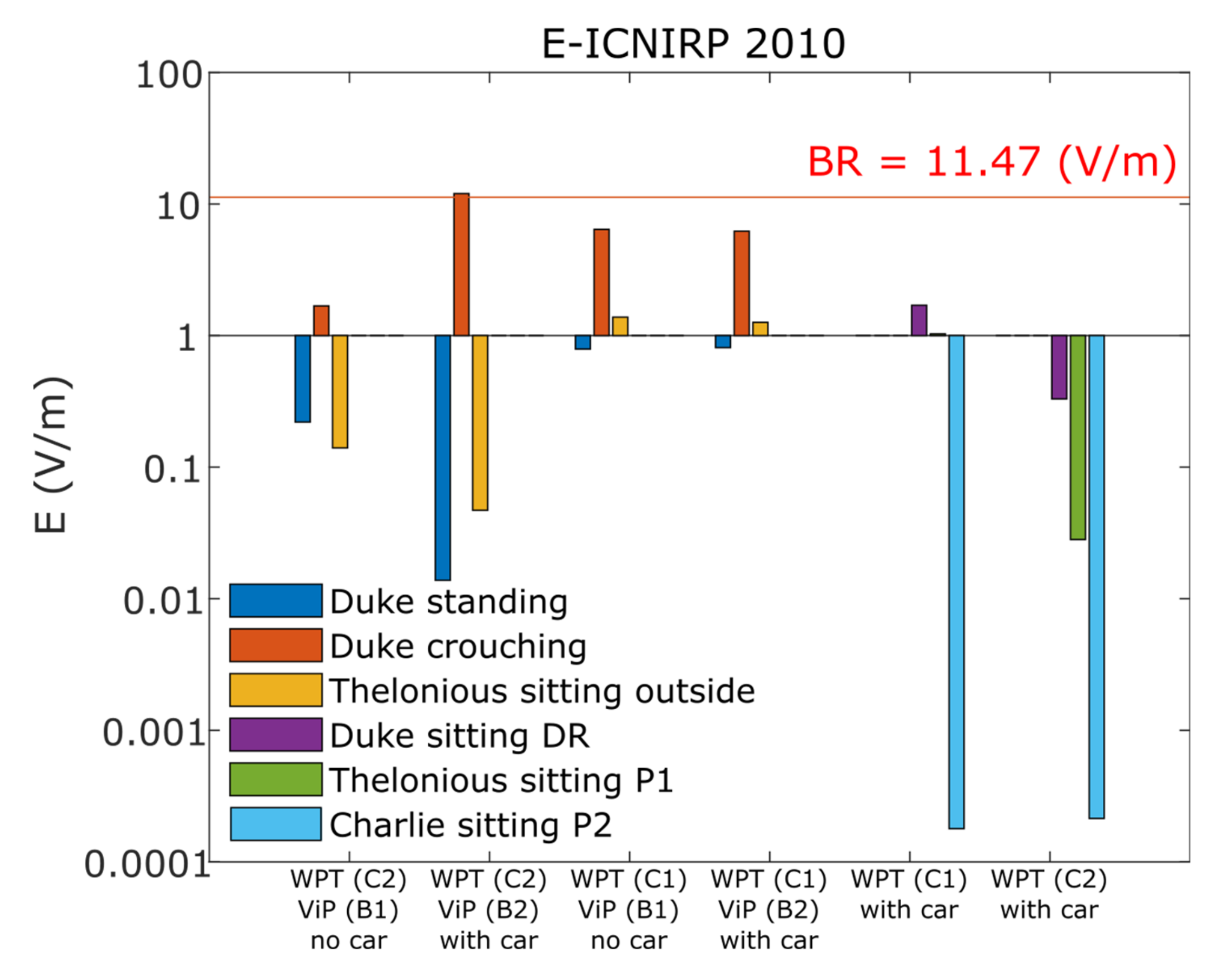
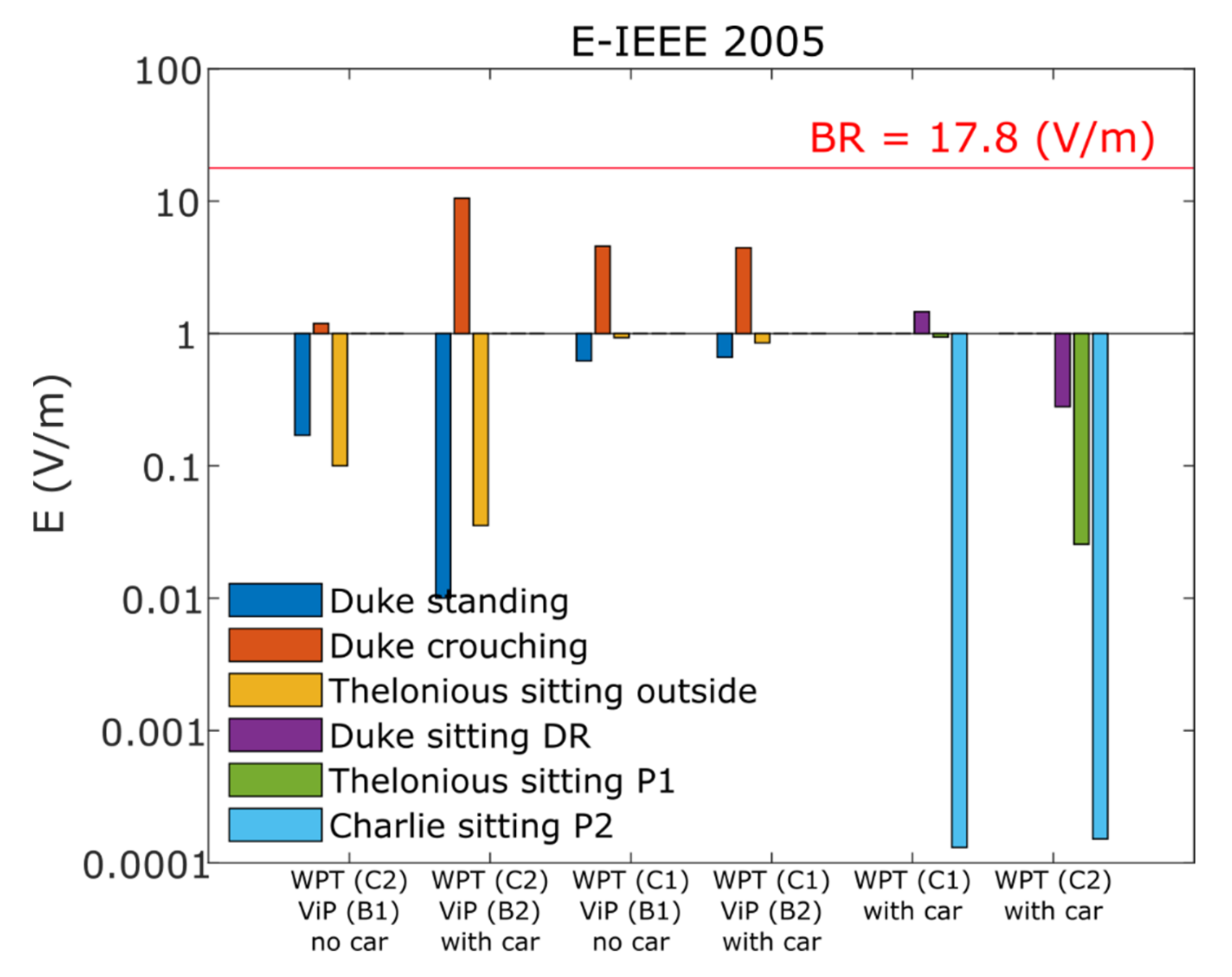
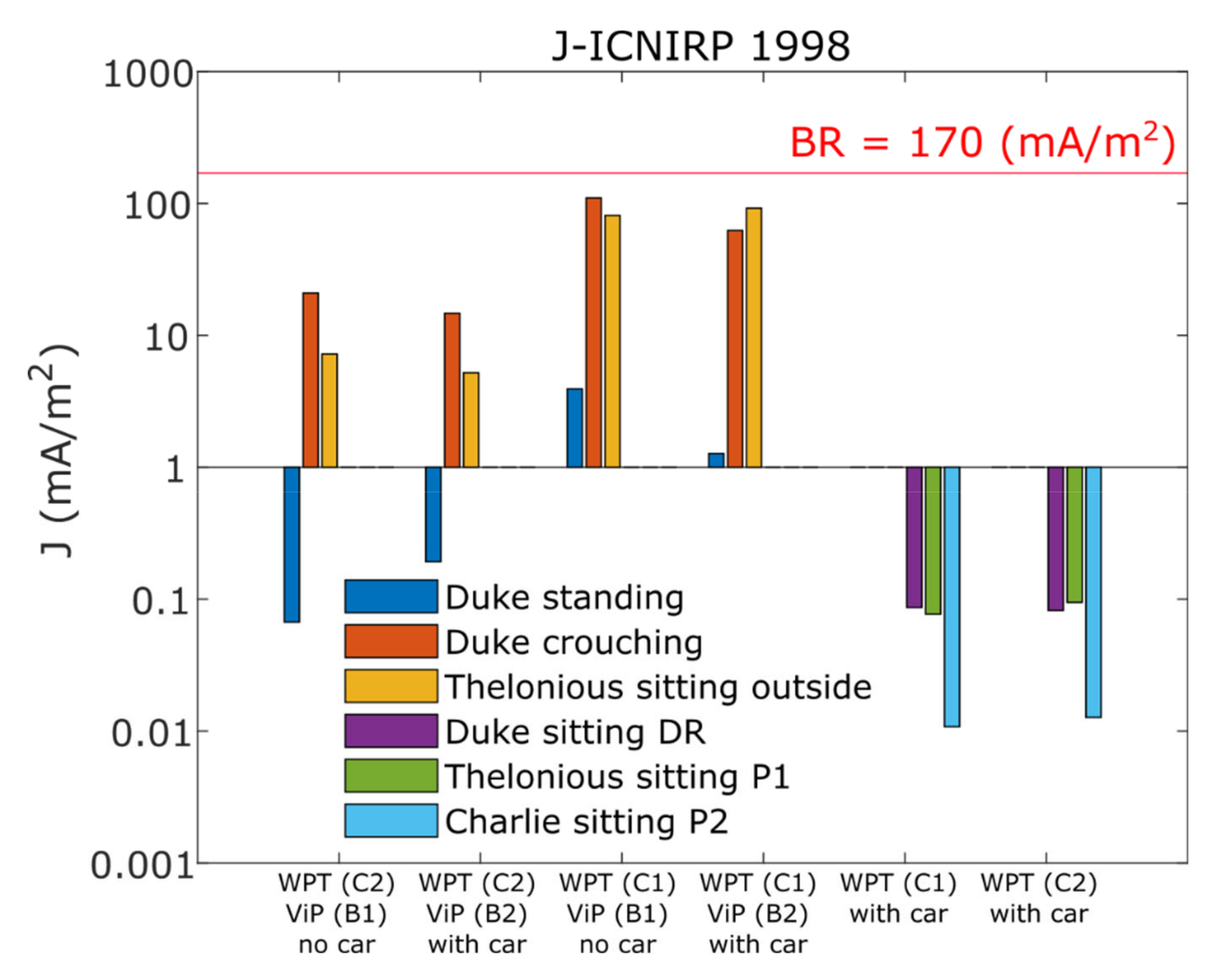
3.2. Numerical Dosimetry of Human Exposure

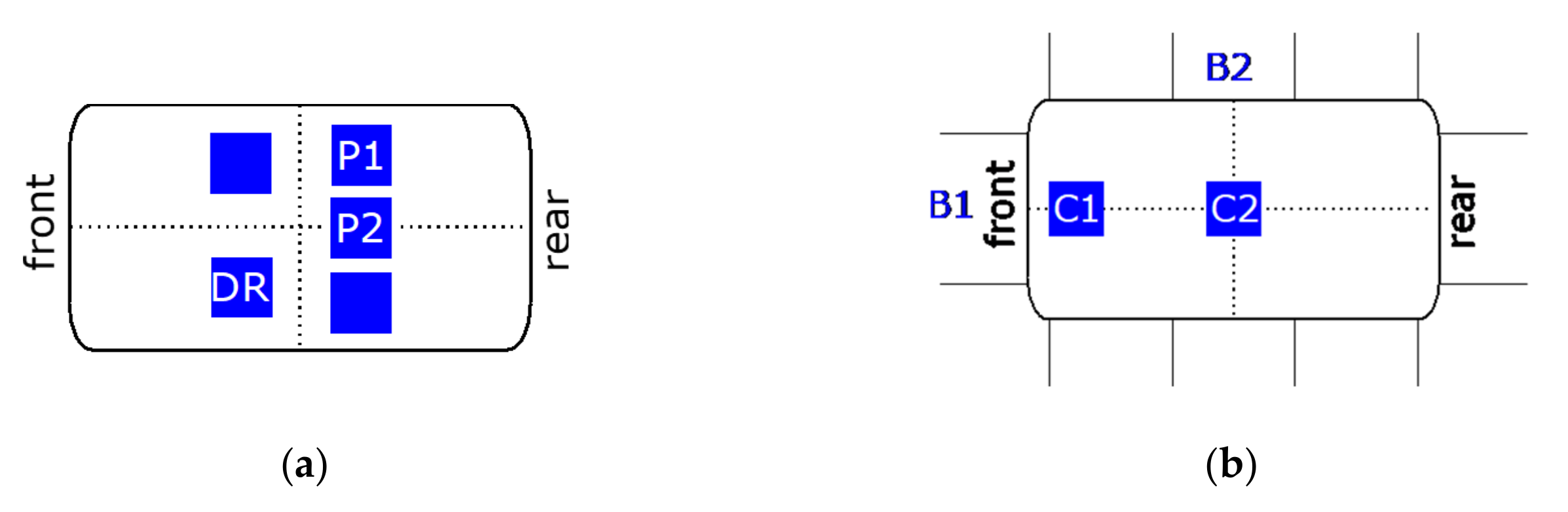
3.2.1. Exposure of the Light EV (The Car)

Figure 17, Figure 18 and Figure 19 show the results related to the exposure scenarios described in Table 5 based on the magnetic field distribution with and without the light EV. The standing posture represents the safest exposure condition for all cases, whereas the induced E-field and current density J approached the BR when the ViP phantoms moved closer to the source, e.g., when the Duke phantom was crouching or when Thelonious was sitting outside the car (Figure 17 and Figure 18).

Considering the passenger safety, the exposure inside the car may be regarded as negligible since all exposures were significantly below the BR levels. However, the levels of induced fields were up to 30 times larger than the BR (data not shown) when Duke was lying on the ground with the arm stretched and the hand very close to the IPT system. This exposure scenario represents an unlikely situation since sensors would detect the presence of living objects in close proximity to the coil and the system would automatically shut down.

3.2.2. Exposure of the Bus

The exposures in proximity to and inside the bus were much lower in all cases than in the light EV, apart from when the Duke model was in the crouching posture outside to the bus.

Table 8. E-fields and current density induced in ViP phantoms due to the magnetic field generated by the IPT system for charging the electric bus for the exposure scenarios described in Table 6.

ViP Model Position	Posture	E-ICNIRP (V/m) (in Bracket the Ratio with Respect to the Limit)	E-IEEE (V/m) (in Bracket the Ratio with Respect to the Limit)	J-ICNIRP (mA/m2) (in Bracket the Ratio with Respect to the Limit)
Carbon-steel alloy bus-body
outside/central	Duke standing	0.3 (0.08)	0.2 (0.03)	4.7 (0.08)
outside/central	Charlie sitting	0.2 (0.05)	0.1 (0.02))	4.2 (0.07)
outside/central	Duke crouching	4.2 (1.12))	3.1 (0.53)	36.8 (0.66)
outside/central	Thelonious sitting	0.6 (0.16)	0.4 (0.07)	76.8 (1.38)
Inside	Duke standing	0.2 (0.05)	0.1 (0.02)	4.3 (0.08)
Inside	Charlie sitting	0.2 (0.05)	0.1 (0.02)	2.6 (0.05)
Fiberglass bus-body
outside/central	Duke standing	0.4 (0.01)	0.3 (0.05)	4.4 (0.08)
outside/central	Charlie sitting	0.2 (0.06)	0.2 (0.03)	5.5 (0.10)

displays the results for the carbon-steel alloy and fiberglass bus-bodies compared with the BR levels for the induced E-field at 27.8 kHz, according to ICNIRP 2010 (BR = 3.75 V/m) and IEEE 2005 (BR = 5.82 V/m) and with the BR level for induced J at 27.8 kHz according to ICNIRP 1998 (BR = 55.6 mA/m²).

The TX coil of the IPT system for charging the bus was placed in the central position and was, therefore, farther away from the ViP phantoms with respect to the previously analyzed exposure conditions. For the fiberglass bus-body, the difference of the induced exposure with respect to the case with metal car-body was up to 35% for the induced E-field and up to 31% for the induced current density J.

4. Discussion

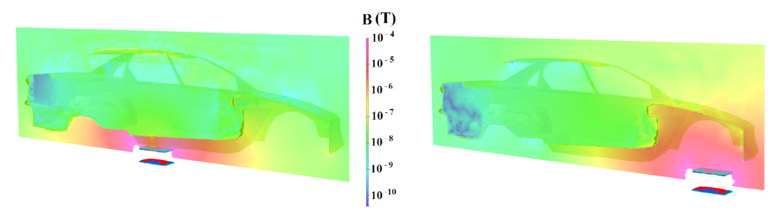
4.1. Magnetic Field Distribution

The accuracy of the charging station modeling was of significant importance for the dosimetric analysis. In this study, the two charging stations were modeled with two previously tested software approaches, along with four other 2D and 3D computational codes on an axisymmetric geometry [22]. In the testing situation presented in [22], the software discrepancies were lower than 6%. For actual geometries, more complex modeling led to higher discrepancies. By carrying out an evaluation of the measurement paths, the average differences between the two computational tools reached values up to 60%.

The results of the simulations were compared with those of the measurement survey carried out on the bus charging station at Zaragoza. The carefully designed survey used both manual positioning for some points (e.g., driver) and positioning lasers. The expanded measurement uncertainty was estimated to be 3.3% (coverage factor k = 2). By excluding some measurement points with anomalous values, even though a simplified model of the minibus was used, the computational tools were able to reproduce the trend of the magnetic induction levels along the measurement paths. This applied even when some discrepancies were present between the simulations and the experiments. The average relative difference between the measurements and the calculated values was in the range of 20–60 %, depending on the investigation area. As shown in Figure 14, Figure 15 and Figure 16, due to the simplification of the bus model, the simulations more accurately reproduced or overestimated the values above 2 μT, while they underestimated the lower induction values.

There are two main reasons for the discrepancies between the measured and simulated results: (i) it was extremely difficult to reproduce the field behavior at the end of the shielding elements, an effect that is particularly apparent near the bus door; (ii) there were uncertainties regarding the position and exact dimensions of the main metallic elements that determine modifications in the field behavior beneath the bus. In addition, the overall worst agreement between the measured and computed results in Session S.3 could be attributed to uncertainties in the accurate estimation of the relative misalignment between the TX and RX coils when moving the bus with respect to the charging station.

Another important outcome of this study is found in the evaluation of the effect of the vehicle-body on the magnetic field around and inside the EV, both for the light EV (car) and the heavy EV (bus).

Referring to the magnetic flux density distribution inside and around the light EV (Figure 10 and Figure 11), the car-body reduces the field outside the EV by four to five orders of magnitude, depending on the area of investigation. The magnetic induction inside the EV is lower than 10 nT near the car-seats, while it rises one order of magnitude (about 100 nT) near the windows. A similar effect is observed for the bus. The peculiar effect of the car-body is highlighted in Figure 11, where it is evident how the shielding effect is weakened at the height of the car-seats when the car door is opened. In this case, the magnetic flux density increases inside the light EV, passing from 2.5 nT to values between 10 nT and 100 nT in the driver’s area. Values lower than 10 nT are comparable to urban environmental noise.

Similar qualitative behavior was found for the bus. As shown in Figure 12, the modeling analysis indicates that the metal floor structure of the bus, together with the aluminum screen and the ferrite concentrators, is able to reduce the external magnetic field generated by the coils by three to four orders of magnitude, depending on the survey area considered. Also, for the bus, it was observed that the magnetic flux density levels tend to increase near to the glass surfaces, particularly near the passenger entrance door, which has larger dimensions compared to common light vehicles. Due to the extensive glass surfaces of the bus, the variation of the B-field between the center of the bus and the glass surfaces was limited to an order of magnitude for the metal bus-body, while the field from the center to one side increased approximately four times for the fiberglass bus-body, as shown in Figure 14 at the floor level. However, passenger exposure remained limited to less than 10% of the basic restrictions, even near the glass surfaces.

4.2. Dosimetric Results

To carry out the dosimetric analysis, the magnetic induction values were calculated with the computational tool that provided fewer discrepancies with respect to the measurements, that is Opera 3D (see Section 3.1). Dosimetric results reported in the present paper and the comparison with limits provided by the current guidelines should be considered with respect to their overall accuracy, as reported in [38].

For the exposure analysis of the light EV (Figure 17, Figure 18 and Figure 19), a unique critical situation was found, with the Duke model crouching outside the EV next to the central charging system. This is a very particular situation that can be easily avoided with sensors that deactivate the coil supply when it occurs. In all other considered situations, both outside the EV (where we always analyzed the worst-case exposure scenarios) and inside the EV, the dosimetric calculations showed negligible exposure, apart from the one where the human model was lying on the ground with the hand stretched out. The car results confirmed what was observed in the dosimetric studies reported in [12,15].

In the case of the dosimetric analysis related to the bus exposure (the results are summarized in Table 8), given the approximations introduced by the bus model and quantified by the discrepancies found in the comparison with measurements, for the specific scenario, a safety factor equal to 3 was adopted to define a situation as safe based on computations. The rationale for choosing the coefficient is given by the maximum discrepancy between measurements and calculations, quantified in Section 3.1 equal to 78%. Therefore, a safety factor of α = 2 could be sufficient to compensate model discrepancies, but a safety factor of α = 3 should be a conservative condition, also considering the measurement uncertainty.

In the conservative case of a fiberglass bus-body, the exposure inside the bus compared to the basic restrictions was 5.3% (15.9%, α = 3) according to ICNIRP 2010, 1.7% (5.1%, α = 3) according to IEEE 2005, and 4.7% (14.1%, α = 3) according to ICNIRP 1998. Considering the assumption of linear dependence and the safety factor, the values of the induced quantities are still well below the basic restrictions. The same applies to most of the other considered positions, where the exposure was always lower than 10% (30%, α = 3) compared to the basic restrictions and, therefore, safe. The only exceptions were the two positions of the Duke crouching and the Thelonious sitting outside the bus near the coils. In the case of the Duke crouching, considering the safety factor, the situation is problematic for all three standards. This is a situation similar to the one found for the car; an issue that could be addressed by a sensor that powers off the system if necessary. With Thelonious sitting, the exposure situation was 16% (48%, α = 3) according to ICNIRP 2010 and 6.9% (20.7%, α = 3) according to IEEE 2005. Applying the safety factor, these situations continue to be safe except for ICNIRP 1998.

5. Conclusions

The results of this study show that IPT charging technology for electric cars can be intrinsically safe. The use of metal vehicle-bodies with a relative magnetic permeability higher than 300, and electrical conductivity of at least 1 MS/m reduces the magnetic induction values inside the vehicle to close to the environmental noise and the exposure levels at least one order of magnitude lower than the basic restrictions. This argues in favor of recharging in car parking lots for taxi drivers for example, or at traffic lights. However, attention must be paid to the following issues: (i) glass surfaces of the vehicles (i.e., windows) must be limited, (ii) the doors should not be opened when charging, (iii) a fiberglass body should not be used. In fact, in all these cases, the driver and passengers tend to increase their exposure, although it appears to remain below the basic restrictions. The same was found for the bus, although its extensive glass surfaces have a lower shielding effect than the vehicle body. Critical situations have been highlighted for both the bus and the car in the event of a driver or passenger crouching or sitting outside the EV, specifically at the side of the EV closest to the coils. In these cases, the exposure exceeds the basic restrictions, and the use of a sensor suitable to power off the system in such circumstances would be warranted.

References

1. Tesla, N. Apparatus for Transmitting Electrical Energy. U.S. Patent 1,119,732, 1 December 1914. [Google Scholar]
2. Kurs, A.; Karalis, A.; Moffatt, R.; Joannopoulos, J.D.; Fisher, P.; Soljačić, M. Wireless Power Transfer via Strongly Coupled Magnetic Resonances. Science 2007, 317, 83–86. [Google Scholar] [CrossRef] [PubMed] [Green Version]
3. Villa, J.L.; Sallán, J.; Llombart, A.; Sanz, J.F. Design of a High Frequency Inductively Coupled Power Transfer System for Electric Vehicle Battery Charge. Appl. Energy 2009, 86, 355–363. [Google Scholar] [CrossRef]
4. El-Shahat, A.; Ayisire, E.; Wu, Y.; Rahman, M.; Nelms, D. Electric Vehicles Wireless Power Transfer State-of-The-Art. Energy Procedia 2019, 162, 24–37. [Google Scholar] [CrossRef]
5. Beh, T.C.; Imura, T.; Kato, M.; Hori, Y. Basic Study of Improving Efficiency of Wireless Power Transfer via Magnetic Resonance Coupling Based on Impedance Matching. In Proceedings of the 2010 IEEE International Symposium on Industrial Electronics, Bari, Italy, 4–7 July 2010; pp. 2011–2016. [Google Scholar]
6. Jang, Y.J. Survey of the Operation and System Study on Wireless Charging Electric Vehicle Systems. Transp. Res. Part C Emerg. Technol. 2018, 95, 844–866. [Google Scholar] [CrossRef]
7. Christ, A.; Douglas, M.; Nadakuduti, J.; Kuster, N. Assessing Human Exposure to Electromagnetic Fields from Wireless Power Transmission Systems. Proc. IEEE 2013, 101, 1482–1493. [Google Scholar] [CrossRef]
8. Schneider, J. Wireless Power Transfer for Light-Duty Plug-in/Electric Vehicles and Alignment Methodology; SAE Int. J2954 Taskforce; SAE Interanational: Warrendale, PA, USA, 2016. [Google Scholar]
9. ICNIRP Guidelines for Limiting Exposure to Time-Varying Electric, Magnetic, and Electromagnetic Fields (up to 300 GHz). Heal. Phys 1998, 74, 494–522.
10. ICNIRP Guidelines for Limiting Exposure to Time-Varying Electric and Magnetic Fields (1 Hz to 100 kHz). Health Phys. 2010, 99, 818–836.
11. IEEE Standards Coordinating Committee. 28. IEEE Standard for Safety Levels with Respect to Human Exposure to Radio Frequency Electromagnetic Fields, 3kHz to 300GHz; IEEE C95. 1-1991; IEEE Standards Coordinating Committee: Piscataway, NJ, USA, 1992. [Google Scholar]
12. Liorni, I.; Lisewski, T.; Capstick, M.H.; Kuehn, S.; Neufeld, E.; Kuster, N. Novel Method and Procedure for Evaluating Compliance of Sources with Strong Gradient Magnetic Fields Such as Wireless Power Transfer Systems. IEEE Trans. Electromagn. Compat. 2019. (Early Access). [Google Scholar] [CrossRef]
13. Park, S. Evaluation of Electromagnetic Exposure During 85 kHz Wireless Power Transfer for Electric Vehicles. IEEE Trans. Magn. 2018, 54, 5100208. [Google Scholar] [CrossRef]
14. Laakso, I.; Hirata, A. Evaluation of the Induced Electric Field and Compliance Procedure for a Wireless Power Transfer System in an Electrical Vehicle. Phys. Med. Biol. 2013, 58, 7583. [Google Scholar] [CrossRef] [PubMed] [Green Version]
15. Shimamoto, T.; Laakso, I.; Hirata, A. In-Situ Electric Field in Human Body Model in Different Postures for Wireless Power Transfer System in an Electrical Vehicle. Phys. Med. Biol. 2014, 60, 163. [Google Scholar] [CrossRef] [PubMed]
16. De Santis, V.; Campi, T.; Cruciani, S.; Laakso, I.; Feliziani, M. Assessment of the Induced Electric Fields in a Carbon-Fiber Electrical Vehicle Equipped with a Wireless Power Transfer System. Energies 2018, 11, 684. [Google Scholar] [CrossRef] [Green Version]
17. Miwa, K.; Takenaka, T.; Hirata, A. Electromagnetic Dosimetry and Compliance for Wireless Power Transfer Systems in Vehicles. IEEE Trans. Electromagn. Compat. 2019, 61, 2024–2030. [Google Scholar] [CrossRef]
18. Wang, Q.; Li, W.; Kang, J.; Wang, Y. Electromagnetic Safety Evaluation and Protection Methods for a Wireless Charging System in an Electric Vehicle. IEEE Trans. Electromagn. Compat. 2019, 61, 1913–1925. [Google Scholar] [CrossRef]
19. Wen, F.; Huang, X. Human Exposure to Electromagnetic Fields from Parallel Wireless Power Transfer Systems. Int. J. Environ. Res. Public Health 2017, 14, 157. [Google Scholar] [CrossRef]
20. Chakarothai, J.; Wake, K.; Arima, T.; Watanabe, S.; Uno, T. Exposure Evaluation of an Actual Wireless Power Transfer System for an Electric Vehicle With Near-Field Measurement. IEEE Trans. Microw. Theory Tech. 2018, 66, 1543–1552. [Google Scholar] [CrossRef]
21. Cirimele, V.; Freschi, F.; Giaccone, L.; Pichon, L.; Repetto, M. Human Exposure Assessment in Dynamic Inductive Power Transfer for Automotive Applications. IEEE Trans. Magn. 2017, 53, 1–4. [Google Scholar] [CrossRef]
22. Zucca, M.; Bottauscio, O.; Harmon, S.; Guilizzoni, R.; Schilling, F.; Schmidt, M.; Ankarson, P.; Bergsten, T.; Tammi, K.; Sainio, P. Metrology for Inductive Charging of Electric Vehicles (MICEV). In Proceedings of the International Conference of Electrical and Electronic Technologies for Automotive 2019 (Aeit Automotive), Torino, Italy, 2–4 July 2019; pp. 1–4. [Google Scholar]
23. Christ, A.; Kainz, W.; Hahn, E.G.; Honegger, K.; Zefferer, M.; Neufeld, E.; Rascher, W.; Janka, R.; Bautz, W.; Chen, J. The Virtual Family—Development of Surface-Based Anatomical Models of Two Adults and Two Children for Dosimetric Simulations. Phys. Med. Biol. 2009, 55, N23. [Google Scholar] [CrossRef]
24. Gosselin, M.-C.; Neufeld, E.; Moser, H.; Huber, E.; Farcito, S.; Gerber, L.; Jedensjö, M.; Hilber, I.; Di Gennaro, F.; Lloyd, B. Development of a New Generation of High-Resolution Anatomical Models for Medical Device Evaluation: The Virtual Population 3.0. Phys. Med. Biol. 2014, 59, 5287. [Google Scholar] [CrossRef] [PubMed]
25. EN Standard 62233:2008, Measurement Methods for Electromagnetic Fields of Household Appliances and Similar Apparatus with Regard to Human Exposure. Available online: https://webstore.iec.ch/publication/6618 (accessed on 3 June 2020).
26. Bottauscio, O.; Chiampi, M.; Crotti, G.; Zucca, M. Probe influence on the measurement accuracy of non-uniform LF magnetic fields. IEEE Trans. Instrum. Meas. 2005, 54, 722–726. [Google Scholar] [CrossRef]
27. Chiampi, G.; Crotti, D. Giordano. Set up and characterization of a system for the generation of reference magnetic fields, from 1 to 100 kHz. IEEE Trans. Instrum. Meas. 2007, 564, 300–304. [Google Scholar] [CrossRef]
28. Zucca, M.; Squillari, P.; Pogliano, U. A Measurement System for the Characterization of Wireless Charging Stations for Electric Vehicles, accepted for presentation to CPEM Conference; Denver, CO, USA. 2020. [Google Scholar]
29. Li, F.; Ferguson, R.; Hart, D.; Guilizzoni, R.; Fatadin, I.; Harmon, S. Characterisation of an optical 2D tracking system. In Proceedings of the of IEEE British and Irish Conference on Optics and Photonics, London, UK, 11–13 December 2019. [Google Scholar]
30. Taylor, B.N.; Kuyatt, C.E. Guidelines for Evaluating and Expressing the Uncertainty of NIST Measurement Results; Physics Laboratory National Institute of Standards and Technology Gaithersburg: Gaithersburg, MD, USA, 1994. [Google Scholar]
31. JCGM. JCGM 100-2008: Evaluation of Measurement Data–Guide to the Expression of Uncertainty in Measurements; Bureau International des Pois et Mesures (BIPM): Sevres, France, 2008. [Google Scholar]
32. Simulia, OPERA. 2020. Available online: https://www.3ds.com/products-services/simulia/products/opera/solutions/ (accessed on 14 April 2020).
33. Simulia, CST. Available online: https://www.3ds.com/products-services/simulia/products/cst-studio-suite/electromagnetic-systems/ (accessed on 14 April 2020).
34. Hasgall, P.A.; Neufeld, E.; Gosselin, M.C.; Klingenböck, A.; Kuster, N.; Hasgall, P.; Gosselin, M. IT’IS Database for Thermal and Electromagnetic Parameters of Biological Tissues. 2012. Available online: https://www.scienceopen.com/document?vid=a95fbaa4-efd8-429a-a59e-5e208fea2e45 (accessed on 3 June 2020).
35. Kuster, N.; Torres, V.B.; Nikoloski, N.; Frauscher, M.; Kainz, W. Methodology of Detailed Dosimetry and Treatment of Uncertainty and Variations for in Vivo Studies. Bioelectromagnetics 2006, 27, 378–391. [Google Scholar] [CrossRef]
36. ZMT, Sim4Life-v5.0. Available online: https://zmt.swiss/news-and-events/news/sim4life/sim4life-major-release-v5-0 (accessed on 14 April 2020).
37. ICNIRP. Guidelines for limiting exposure to electromagnetic fields (100 kHz to 300 GHz). Health Phys. 2020, 118, 483–524. [Google Scholar] [CrossRef]
38. Arduino, A.; Bottauscio, O.; Chiampi, M.; Giaccone, L.; Liorni, I.; Kuster, N.; Zilberti, L.; Zucca, M. Accuracy Assessment of Numerical Dosimetry for the Evaluation of Human Exposure to Electric Vehicle Inductive Charging Systems. IEEE Trans. Electromagn. Compat. 2020. [Google Scholar] [CrossRef]
Figure 1. (a) Relative location of the transmitting and receiving coils of the minibus charging station, (b) Bus approaching the coil pad, (c) Image of the transmitting coil, (d) Image of the receiving coil located under the bus.
Sustainability 12 04573 g001
Figure 2. Block diagram of the bus IPT system tested. Ground side: the first block comprises one IGBT-based AC/DC grid multilevel converter, an internal 700 V DC bus, and one DC/DC buck converter. Block 2 corresponds to a variable DC bus (ranging from 70 V to 500 V). The third block includes a DC to AC high-frequency H-bridge converter that feeds Block 4, the primary Series-Parallel resonant tank. Vehicle side (inside the vehicle): secondary Series resonant tank (Block 5), AC high-frequency to DC secondary converter (Block 6) that filters and converts, EV batteries (Block 7).
Sustainability 12 04573 g002
Figure 3. (a) S80 Volvo car-body cross-section and location of the coil charging system; (b) complete car-body and charging coils in front of the car and (c) coil pad constructed according to the SAE J2954 standard.
Sustainability 12 04573 g003
Figure 4. Probe configuration of the ELT-400 coil probe configuration. The arrangement of the coils well suited for the calibration operations. [Source: Narda Safety Test Solutions ELT-400 Operating Manual].
Sustainability 12 04573 g004
Figure 5. Configuration of the magnetic unit, which is part of the Power Measurement Unit (PwMU). Main hardware components: Narda ELT-400 field meter, VGA-BNC cable, two synchronized NI PXI 5922 oscilloscope cards measuring the field components from the meter analog output, PXI NI 6683 H GPS synchronization module, GPS antenna and cable, laptop with LabVIEW software controlling data acquisition and storage.
Sustainability 12 04573 g005
Figure 6. (a) The minibus during measurements; (b) the minibus internal floor with the meters for electromagnetic measurements, the positioning system, and, in the inset, the data acquisition system and control.
Sustainability 12 04573 g006
Figure 7. Schematic of the centered position of the WPT system, together with the adopted reference coordinate system. In the misaligned case, the system is the same, but the bus (and, therefore, the receiving coil) is transferred by a distance equal to 0.843 m along the y direction.
Sustainability 12 04573 g007
Figure 8. Sketch of the bus (heavy vehicle) viewed from the top, with locations of the measurement points for the three sessions. The black dashed line represents data for session S.1, and the red dashed line corresponds to data for session S.3 (only the first height, for measurement ID 1 to 12, is shown for simplicity). Measurement positions for session S.2 are identified by the passengers (Pn), bystander (B), and driver (D) markers.
Sustainability 12 04573 g008
Figure 9. (a) General representation of possible positions of the human body models sitting inside the light EV (P1, P2, DR), (b) the general position of the coil under the light EV (C1 and C2) and of the human body models outside the car (B1 and B2).
Sustainability 12 04573 g009
Figure 10. Magnetic induction behavior on a plane corresponding to the median section of the car-body. The central charging coils are shown on the left, and the charging coils at the front of the car are shown on the right.
Sustainability 12 04573 g010
Figure 11. The effect of the door opening on the central IPT. The maps of the B-field amplitude are reported at the height z = 0.4 m: (a) with closed door, (b) with open door.
Sustainability 12 04573 g011
Figure 12. (a) Overall view of the bus models with a part of the volume mesh formed around the bus-body. The receiver coil and the transmitter coil are visible in red. (b) Structure of the bus charging coils and the equivalent structure of the bus from the electromagnetic point of view. (c,d) Magnetic flux density distribution in a vertical cross-section in the middle of the bus: (c) with centered coils, (d) with coils misaligned by 0.843 m.
Sustainability 12 04573 g012
Figure 13. Spatial distribution of the measured B-field amplitude for session S.1 at the bus floor level (a) and for a vertical plane corresponding to the bus entrance in session S.3 (b). The coordinates (x, y, z) here reported corresponding to the reference system introduced in Figure 7 and Figure 8. The two figures have the same geometrical scales.
Sustainability 12 04573 g013
Figure 14. Comparison between measured and simulated B-field values for session S.1 at the bus floor. Refer to Figure 8 for the position of the measurement points. Maximum discrepancies between measured and computed values are highlighted in the plot with dashed circles.
Sustainability 12 04573 g014
Figure 15. Comparison between measured and simulated B-field values for session S.2. Refer to Figure 8 for the position of the measurement points. Maximum discrepancies between the measured and computed values are highlighted in the plot with dashed circles.
Sustainability 12 04573 g015
Figure 16. Comparison between measured and simulated B-field values for session S.3. Refer to Figure 8 for the position of the measurement points. Two sets of twelve measurement points are plotted for two heights h from the ground floor. Maximum discrepancies between the measured and computed values are highlighted in the plot with dashed circles.
Sustainability 12 04573 g016
Figure 17. Peak of the E-field (V/m) averaged according to ICNIRP 2010 guidelines induced in the ViP phantoms for the exposure scenarios described in Table 5. The horizontal red line represents the BR level for induced E-field at 85 kHz, according to ICNIRP 2010.
Sustainability 12 04573 g017
Figure 18. Peak of the E-field (V/m) averaged according to IEEE 2005 guidelines induced in the ViP phantoms for the exposure scenarios described in Table 5. The horizontal red line represents the BR level for induced E-field at 85 kHz, according to IEEE 2005.
Sustainability 12 04573 g018
Figure 19. Peak of the J current (mA/m2) averaged according to ICNIRP 1998 guidelines induced in the central nervous system of the ViP phantoms for the exposure scenarios described in Table 5. The horizontal red line represents the BR level for induced J at 85 kHz, according to ICNIRP 1998.
Sustainability 12 04573 g019