Joint Probabilistic Modeling of Wind Speed and Wind Direction for Wind Energy Analysis: A Case Study in Humansdorp and Noupoort

Abstract

South Africa has great potential for considering wind energy as an alternative resource. The climatology allows for significant wind energy production. An accurate joint description of the wind speed (linear) and wind direction (circular) characteristics is important for wind farm development. In this paper, a bivariate class of flexible joint probability density functions of wind speed and wind direction for the use in wind energy analysis is presented. This joint model accounts for bimodality, skewness, and a dependency structure between the wind speed and wind direction. For the joint probabilistic description of the wind speed and wind direction, special cases of this bivariate class are evaluated, namely the semi-parametric Möbius model on the disc, the Möbius distribution on the disc, and the Beta type III Möbius distribution on the disc. These three special cases are applied to wind speed and wind direction data recorded every ten minutes at two locations in South Africa. Evaluation of the models is based on three different information criteria and normalized deviation. Overall, the semi-parametric model is superior to the parametric models based on the performance measures. The wind energy potential at the two locations is evaluated using the semi-parametric model.

1. Introduction

In South Africa, fossil fuels are the main form of energy supply. This results in emissions causing local and global environmental complications. Fossil fuels are not sustainable and, therefore, it is of importance to investigate renewable energy resources. Eskom (the electricity supply commission of SA) is a South African electricity public utility that generates approximately 95% of electricity used in South Africa. It is also well known that Eskom’s current fleet of power stations is old and suffers from reliability problems, resulting in frequent load shedding (a controlled blackout to respond to unplanned events to protect the electricity power system from a total blackout), with a negative impact on the South African economy. Renewable resources also have inherent constraints; for example, solar power is limited to the availability of the sun rays and is costly. Considering the climatology of South Africa, wind energy stands out as a viable option. From an environmental impact perspective, wind energy is superior in comparison to other energy sources [1]. As reported by [1], even though wind energy is popular due to the cost efficiency, there are some unfavorable environmental impacts of wind energy, such as the noise produced by the windmills, its impact on the ecology (bird hits), etc. To overcome these negative impacts, the design of the wind farms is of utmost importance.

The overall capacity of all wind turbines installed worldwide reached 597 GW by the end of 2018 (Global Wind Energy Council: Global wind statistics, 2019; https://gwec.net/wp-content/uploads/2019/04/GWEC-Global-Wind-Report-2018.pdf (accessed 22 August 2019)). This covers 6% of the global electricity demand. As emphasized in [2], a total of 98 countries can be provided with electricity produced by wind energy. Furthermore, there is a great interest in expanding wind energy. Modeling of short-term wind speed is essential for evaluating wind energy potential. Typical distributions that are used in characterizing wind speed observations are Weibull, gamma, normal, Rayleigh, log-normal, Nakagami, inverse Gaussian, logistic, and Birnbaum–Saunders distributions. A review of the different distributions used to model wind speed is given in [3]. Apart from wind speed, the importance of including wind direction in the analysis of wind energy has been emphasized in many studies [4,5,6,7,8,9,10,11,12,13,14]. According to [15], existing wind distributions can be classified into two groups: (i) Unimodal and univariate distributions of wind speed and (ii) unimodal and bivariate distributions of wind speed and wind direction. The use of a joint probability density function (PDF) of wind speed (linear variable) and wind direction (circular variable) is important in wind energy projects [4]. In this paper, a flexible joint PDF of wind speed and wind direction is presented using the disc manifold, which has an embedded correlation structure for the circular–linear variables. Current bivariate models for wind speed and wind direction have all been defined on a cylindrical manifold. A comprehensive summary of circular–linear distributions on the cylindrical manifold can be found in [16]. Unlike the widely used Johnson–Wehrly (JW) [17] construction method used in [4,10,11,13,18,19,20], this class of distributions allows for the joint modeling of wind speed and wind direction with an integrated correlation structure. In this paper, we will only focus on models defined on the disc, as a comparison with cylindrical models is invalid due to the different manifolds. Furthermore, this proposed class of distributions accounts for bimodality and skewness present in the data. Thus, the practitioner can more accurately model the wind power density [21] for determining wind farm locations and optimal wind energy potential at various locations.

The remainder of this paper is organized as follows: Section 2 provides background and describes the wind data recorded at two locations in South Africa, namely Humansdorp and Noupoort. The proposed wind models are presented in Section 3. In Section 4, the methodology for finding the estimated values of the parameters of the underlying statistical distributions is discussed. The fitting criteria implemented in the evaluation of the bivariate fits are outlined. The numerical results are presented in Section 5, and Section 6 concludes with some final remarks.

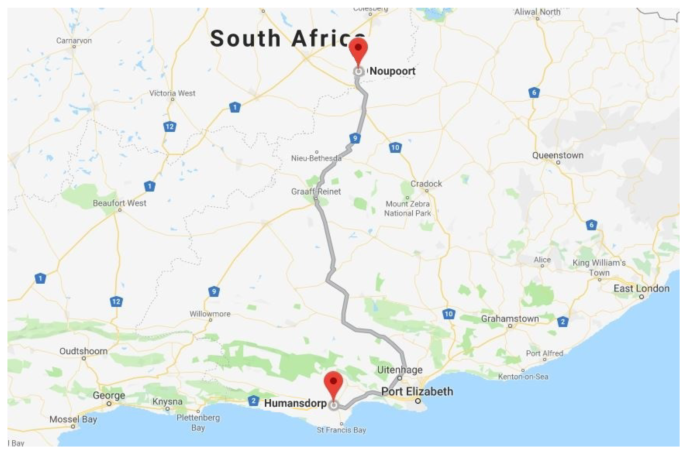
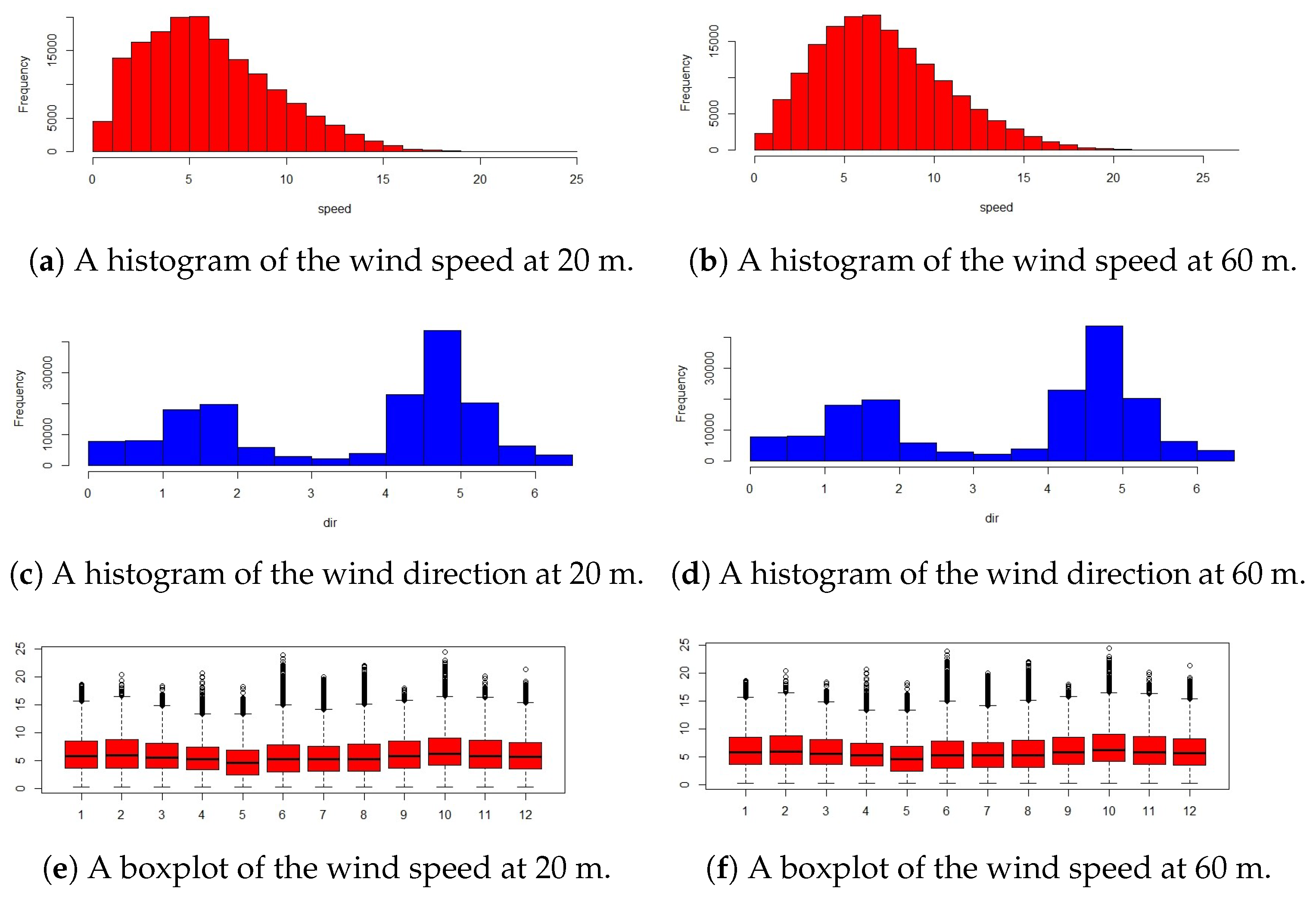
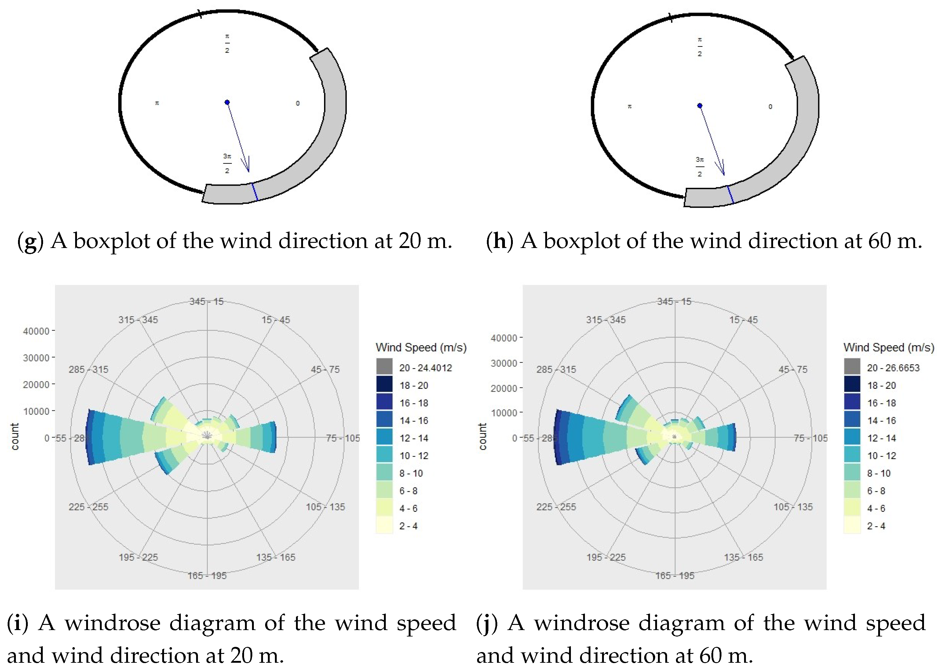
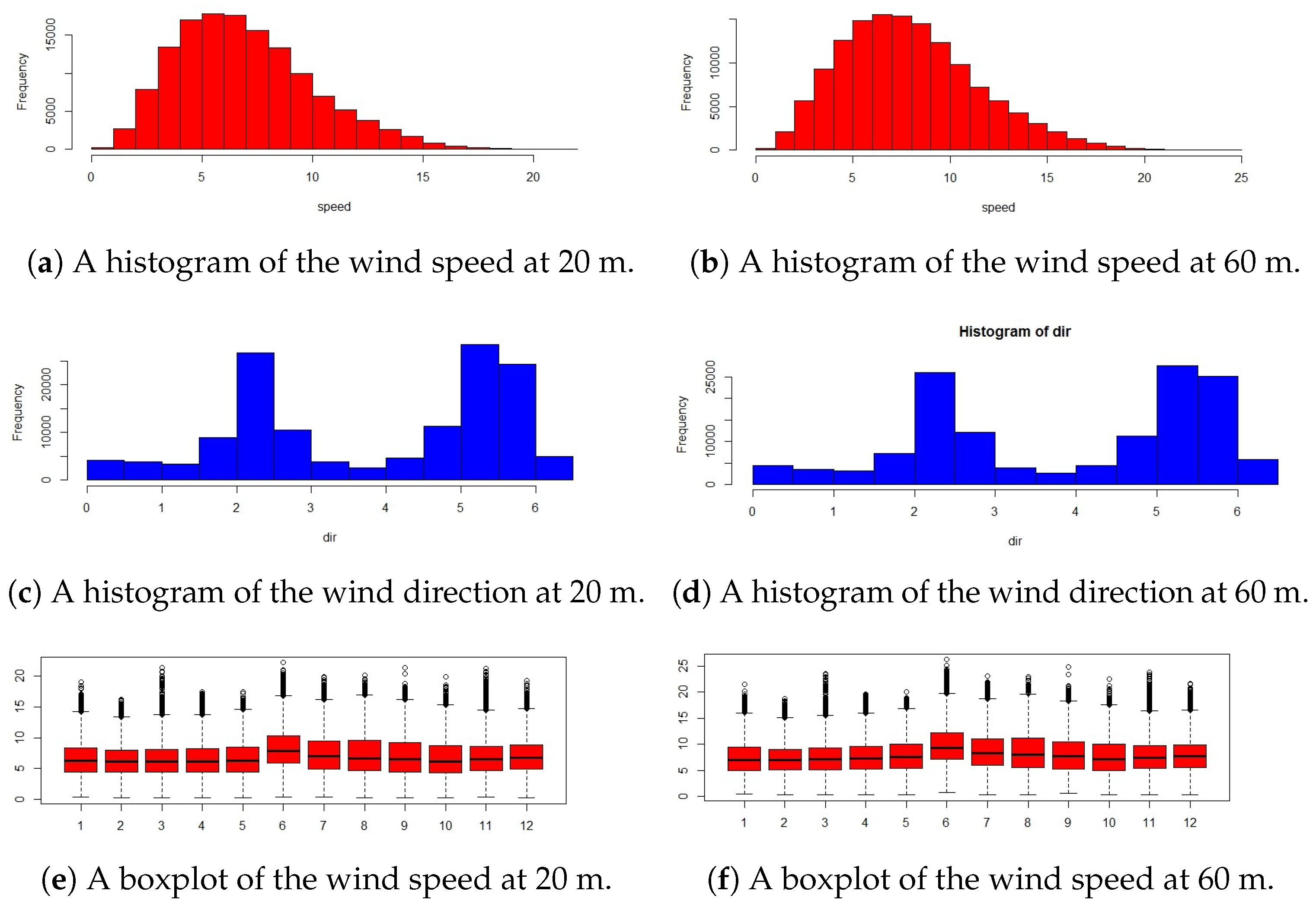
2. Site Location and Wind Data

As of 2019, in South Africa, there are 33 wind farms: 22 fully operational and 11 in construction (based on the South African Wind Energy Association https://sawea.org.za/). In order to assess the competence of the proposed models, two stations situated in South Africa, namely Humansdorp and Noupoort, have been selected. These locations already have a fully operational wind farm; however, they were chosen due to the availability of data. The wind speed and wind direction provided by the Wind Atlas for South Africa project (WASA) (http://wasadata.csir.co.za/wasa1/WASAData (accessed 29 August 2019)) were recorded every 10 min at 20 and 60 m heights. For each location, the main characteristics were reported by the WASA (http://stel-apps.csir.co.za/wasa-data/docs/WASA1Station_and_Site_Description_Report_April2014.pdf (accessed 29 August 2019)); these characteristics include a photographic documentation of mast design, installation, and surroundings, as well as elevation maps that have been constructed for each site from Shuttle Radar Topography Mission (SRTM) 3 arc-second data. These reported images provide an overall view of the location and terrain. Figure 1 shows the locations of the stations and

Table 1. Geographical details of the two stations.

Station	Latitude	Longitude	Elevation
	(${}^{\circ }$S)	(${}^{\circ }$E)	(m)
Humansdorp	−34.109965	24.514360	110
Noupoort	31.252540	25.028380	1806

provides the geographical details for the locations.

In

Table 2. Information of the wind data for the two locations.

Station	Data Period (dd/mm/yyyy)	Total Data	Expected Data	Absent Data
Humansdorp	01/01/2016–28/02/2019	166,226	166,320	94
Noupoort	01/01/2016–28/02/2019	137,660	166,320	28,660

, information on the quantity and quality of the measured wind data for the two locations is given. The period of utilized data, the total number of observations, the number of expected data, and absent data are presented, respectively. The record contained no calm data, as the average of the wind speed over a ten-minute interval was recorded.

In

Table 3. Descriptive statistics of the wind speed data.

Station	Height (m)	Max (m/s)	Mean (m/s)	std (m/s)	Skewness	Kurtosis
Humansdorp	20	24.40	6.01	3.40	0.68	0.16
Humansdorp	60	26.66	7.13	3.65	0.63	0.26
Noupoort	20	21.37	6.93	3.09	0.64	0.19
Noupoort	60	24.79	7.91	3.50	0.57	0.13

, the descriptive statistics for the wind speed for the two locations are given; specifically, the maximum (Max), mean, standard deviation (std), skewness, and kurtosis (skewness is a measure of the asymmetry, and kurtosis measures the peakedness of the distribution). In 

Table 4. Descriptive circular statistics for the wind direction data.

Station	Height (m)	$\overline{\mathit{\omega }}$	$\overline{\mathit{\theta }}$ (rad)	${\mathit{V}}_{\mathit{\Theta }}$	${\mathit{\nu }}_{\mathit{\Theta }}$	$\mathit{\delta }$	s	k
Humansdorp	20	0.24	−1.21	0.76	1.68	8.10	0.55	−0.65
Humansdorp	60	0.28	−1.16	0.72	1.60	6.22	0.60	−0.71
Noupoort	20	0.14	−0.82	0.86	1.99	23.92	0.04	−0.72
Noupoort	60	0.15	−0.88	0.85	1.95	20.69	−0.08	−0.74

, the values of the main circular statistics [22] of the wind direction for the two locations are given. Specifically, the mean resultant length ($\overline{\omega }$), mean direction ( $\overline{\theta }$ ), circular variance ($V_{\mathsf{\Theta }}$), circular standard deviation (${\nu }_{\mathsf{\Theta }}$), circular dispersion ($\delta$), circular skewness (s), and circular kurtosis ( k) are shown.

From Table 3, Noupoort has the highest mean wind speed with the value of 7.91 m/s, while Humansdorp has the lowest mean wind speed with the value of 6.01 m/s. Since the skewness is positive for both the stations, we can conclude that the distributions are skewed to the right. The wind direction data for the Humansdorp location seems to be more concentrated based on the $\overline{\omega }$, as seen in Table 4. Based on the $\overline{\theta }$, the Humansdorp location is dominated by winds blowing from the West-Northwesterly (for $\theta \in [1.77;2.16]$) sector while for Noupoort the dominant wind direction is North Westerly (for $\theta \in [1.57;2.36]$).

3. Models

Based on the assumption that the air density (air density is dependent on altitude, humidity, and temperature; we consider the air density to be independent of the wind characteristics and be equal to a constant value of 1.225 kg/m${}^3$), $\rho$, is constant, the wind power probability density function is expressed as [4]

$$P(x,\theta )=\frac{1}{2}\rho f_{X,\mathsf{\Theta }}(x,\theta )x^3.$$

(1)

The wind power density defined in (1) is used to evaluate the wind energy at the two locations.

Consider the following joint PDF for the wind speed, X, and the wind direction, $\mathsf{\Theta }$, namely the General Möbius distribution on the disc (GM) [23],

$$f_{X,\mathsf{\Theta }}(x,\theta )=\frac{C{\left(1-a^2\right)}^{2}x}{\pi {\left[1-2axcos\left(\theta -\mu \right)+a^2{x}^2\right]}^2}g\left(\frac{a^2-2axcos\left(\theta -\mu \right)+x^2}{1-2axcos\left(\theta -\mu \right)+a^2{x}^2}\right),$$

(2)

with $a\in [0,1)$, $\mu \in (-\pi ,\pi ]$ and $x\in [0,1]$, $\theta \in (-\pi ,\pi ]$, $g(·)$ is a continuous function with support $[0,1]$, and

$$C={\left[\pi \sum _{k=0}^{\infty }\frac{g^{\left(k\right)}\left(0\right)}{(k+1)!}\right]}^{-1},$$

where $g^{\left(k\right)}(·)$ denotes the derivatives of $g(·)$ around zero. We denote this class as $\left(X,\theta \right)\sim GM\left(\mathsf{\Psi },g\right)$ where the set of parameters is denoted by $\mathsf{\Psi }$ with $\mathsf{\Psi }=(a,\mu )$. The parameters can be interpreted as a controlling the skewness, or the asymmetry for the length from the center of the disc, and $\mu$ controlling the orientation of the distribution.

Using the results of [23], we present the following three special models of (2), namely (i) a semi-parametric Möbius model on the disc (SPM), (ii) the Möbius distribution on the disc (MD), and (iii) the Beta type III Möbius distribution on the disc (BM), to jointly model the wind speed and wind direction for the wind data observed at Humansdorp and Noupoort. The parametric special cases are obtained by considering the form of the function $g(·)$ to be as given in

Table 5. Form of $g(·)$ considered for the parametric special cases.

Model	$\mathit{g}\left(\mathit{w}\right)$	Parameter Conditions
MD	${\left(1-w\right)}^{\gamma -1}$	$\gamma \in (0,\infty )$
BM	$w^{\beta -1}{\left(1-w\right)}^{\gamma -1}{\left(1+w\right)}^{-(\gamma +\beta )}$	$\gamma \in (0,\infty )$, $\beta \in (0,\infty )$

. By substituting the form of $g(·)$ in (2), we obtain the joint PDF of the proposed models, as given in

Table 6. Proposed joint probability density functions (PDFs) used for the joint modeling of wind speed and wind direction.

Distribution	Probability Density Function	Domain of Definition	$\mathsf{\Psi }$	Parameter Conditions
SPM	$f\left(x,\theta \right)=\frac{C{\left(1-a^2\right)}^{2}x}{\pi {\left[1-2axcos\left(\theta -\mu \right)+a^2{x}^2\right]}^2}g\left(\frac{a^2-2axcos\left(\theta -\mu \right)+x^2}{1-2axcos\left(\theta -\mu \right)+a^2{x}^2}\right)$	$x\in [0,1]$, $\theta \in (-\pi ,\pi ]$	$\{a,\mu \}$	$a\in [0,1)$, $\mu \in (-\pi ,\pi ]$
	where $C={\left[\pi {\sum }_{k=0}^{\infty }\frac{g^{\left(k\right)}\left(0\right)}{(k+1)!}\right]}^{-1}$	$g(·)$ is a continuous function with support $[0,1]$
MD	$f\left(x,\theta \right)=\frac{\gamma {\left(1-a^2\right)}^{\gamma +1}x{\left(1-x^2\right)}^{\gamma -1}}{\pi {\left(1-2axcos\left(\theta -\mu \right)+a^2{x}^2\right)}^{\gamma +1}},$	$x\in [0,1]$, $\theta \in (-\pi ,\pi ]$	$\{a,\mu ,\gamma \}$	$a\in [0,1)$, $\mu \in (-\pi ,\pi ]$, $\gamma \in (0,\infty )$
BM	$f\left(x,\theta \right)=\frac{2^{\beta }\mathsf{\Gamma }\left(\beta +\gamma \right){\left(1-a^2\right)}^{\gamma +1}x{\left(1-x^2\right)}^{\gamma -1}{\left[a^2-2axcos\left(\theta -\mu \right)+x^2\right]}^{\beta -1}}{\pi \mathsf{\Gamma }\left(\beta \right)\mathsf{\Gamma }\left(\gamma \right){\left[\left(1+x^2\right)\left(1+a^2\right)-4axcos\left(\theta -\mu \right)\right]}^{\gamma +\beta }},$	$x\in [0,1]$, $\theta \in (-\pi ,\pi ]$	$\{a,\mu ,\gamma ,\beta \}$	$a\in [0,1)$, $\mu \in (-\pi ,\pi ]$, $\gamma \in (0,\infty )$, $\beta \in (0,\infty )$

.

The parameters in the MD and BM models can be interpreted as $\gamma$ controlling the steepness of the concentration and $\beta$ contributing to the concentration by adding bimodality. As the value of $\beta$ increases ($\beta >1$), the model introduces another mode in the form of an antimode. The behavior of the parameters is discussed in [23].

4. Materials and Methods

4.1. Fitting of the System of Wind Distributions

For the estimation of the parameters of the SPM model, the computational stages for estimating $g(·)$ and the parameters are given by Algorithm 1. For the parameter estimation of the MD and BM models, maximum likelihood (ML) estimation is performed. Since closed-form expressions could not be obtained for the parameters, numerical optimization of the ML is performed using the "optimization" package available in the R software.

A general algorithm for estimating the parameters of the SPM model is given in [23]. In this paper, a specific case of the general algorithm was used and is described in Algorithm 1.

Take note that, in Algorithm 1 Step 1, the kernel function is estimated using the argument $x^2$. This was chosen as it is the argument before the Möbius transformation and, since the transformation applies to the variable, the function of $g(·)$ can be estimated using the original argument.

In Algorithm 1, the starting values for a and $\mu$ are obtained using a randomized technique of simulating random numbers for $a\in [0,1)$ and $\mu \in [-\pi ,\pi )$ and selecting the set of parameters, $\widehat{\mathsf{\Psi }}$, that maximize the likelihood function.

4.2. Evaluation of Goodness-of-Fit

In this paper, four goodness-of-fit metrics were applied to evaluate the models. The Akaike information criterion (AIC) estimates the relative amount of information lost by a given model. The Bayesian information criterion (BIC) is widely used for model selection and is similar to the AIC. The Hannan–Quinn information criterion (HQC) is similar to the BIC and is strongly consistent. These three measures differ in terms of the amount of model complexity penalization. The two measures BIC and HQC penalize more severely than AIC [24]. The BIC attempts to find the true model among the set of candidates; however, this is not the case for the AIC [25]. The conclusion made using the AIC and BIC will only differ when the AIC chooses a larger model (more complex model) than the BIC. From a statistical viewpoint, information criteria are commonly used when assessing the accuracy of a probabilistic model [26]. These three strict criteria are considered most significant in measuring performance accuracy of distributions. These three metrics are defined in

Table 7. Evaluated goodness-of-fit metrics.

Metric	Equation
$AIC$	$2p-2ln\left(\widehat{L}\right)$
$BIC$	$p\ln \left(n\right)-2\ln \left(\widehat{L}\right)$
$HQC$	$2p\ln \left[\ln \left(n\right)\right]-2\ln \left(\widehat{L}\right)$

, where p is the number of estimated parameters in the model, n the total number of data points, and $\widehat{L}$ the maximum value of the likelihood function for a specific model.

Algorithm 1 Maximum likelihood (ML) estimation algorithm for semi-parametric Möbius model on the disc (SPM) model.

Step 1. Given the observations $x_1,x_2,\dots ,x_n$, we estimate $g(·)$ in (2) using kernel density estimation as follows: $$\widehat{g}\left(w\right)=\frac{1}{nh}\sum _{i=0}^{n}K\left(\frac{w-w_i}{h}\right),$$ where $w_i=x_i^2$, h is the bandwidth, and $K(·)$ is the kernel function. For this paper, we assume a Gaussian kernel with restricted support of $x\in [0,1]$ and use a plug-in bandwidth selection technique to obtain the optimal h value.      Step 2. For given a and $\mu$, compute the value of the argument of $g(·)$ in (2), i.e., compute the value of $q_i=(a^2-2a{x}_{i}cos\left({\theta }_i-\mu \right)+x_i^2)/(1-2a{x}_{i}cos\left({\theta }_i-\mu \right)+a^2{x}_i^2)$. Using the function estimated in Step 1, $\widehat{g}(·)$, calculate the corresponding function of $\widehat{g}\left(q_i\right)$.      Step 3. Compute the likelihood function based on (2) using the estimated $\widehat{g}\left(q_i\right)$, $\widehat{a}$, and $\widehat{\mu }$.      Step 4. Repeat Steps 2 and 3 using an optimization technique to achieve convergence for the parameters a and $\mu$. The final estimated values are those that maximize the likelihood function.

Remark 1.

It is appropriate to compare parametric with semi-parametric models via AIC or BIC. We can motivate this two ways. The process in this paper of implementing kernel density estimation on the unknown function g(·) and then maximum likelihood estimation on the model is similar to that in [27], where they used the AIC and BIC for model selection in a semi-parametric context. Secondly, from the profile likelihood viewpoint [28], by substituting the estimated g() into the density function (Equation (2)), we obtain a parametric form for which we can then apply maximum likelihood estimation as in [29,30,31].

The fourth goodness-of-fit measure is the normalized deviation, which is used for circular–linear models [4]. The normalized deviation is based on the difference between the observed, $N_{ij}^{\left(o\right)}$, and expected, $n{p}_{ij}^{\left(e\right)}$, number of data points. The expression for the normalized deviation, $d_{ij}$, is given by

$$d_{ij}=\frac{N_{ij}^{\left(o\right)}-n{p}_{ij}^{\left(e\right)}}{{\sigma }_{ij}^{\left(e\right)}},$$

(3)

where ${\sigma }_{ij}^{\left(e\right)}$ is the normalizing factor and the expected standard deviation. Normalized deviation values close to zero indicate a model of good fit.

Remark 2.

On the use of AIC, BIC, and HQC in order to compare parametric and semi-parametric models, one must make some regularity assumptions. As such, we will be assuming the estimation of the nonparametric component $g(·)$ using the kernel density estimation is a finite-dimensional problem in our case. Once we estimate the nonparametric component, we apply the plugin approach into the likelihood (as outlined in Algorithm 1) and then maximize the log likelihood to obtain the estimate of parameters; indeed, this a maximization over a restricted parameter space. There is no guarantee that using this method will provide good estimates for the parameters. Therefore, in order to make sure the estimates fulfill satisfactory conditions, we need to use other measures in addition to the aforementioned information criteria. As such, we computed the normalized deviation for a valid comparison.

4.3. Influence of Wind Speed and Wind Direction Data

The bivariate relationship between the wind speed and wind direction is measured by the linear–circular correlation coefficient, $r_{x,\theta }$, defined in [22] as

$$r_{x,\theta }=\sqrt{\frac{r_{xc}^2+r_{xs}^2-2r_{xc}{r}_{xs}{r}_{cs}}{1-r_{cs}^2}},$$

(4)

where $r_{xc}=cor(x,cos\theta )$, $r_{xs}=cor(x,sin\theta )$, and $r_{cs}=cor(cos\theta ,sin\theta )$. The correlation coefficients for the two locations are given in

Table 8. Correlation coefficient for the wind speed and wind direction.

Station	Height (m)	Correlation Coefficient
Humansdorp	20	0.2487562
Humansdorp	60	0.1711075
Noupoort	20	0.2688977
Noupoort	60	0.2677411

, emphasizing the need for a joint model with an embedded correlation structure.

Subsequently, in Figure 2 and Figure 3, the wind speed and wind direction for the two locations are given to assist the practitioner in choosing an appropriate model. Figure 2a–d and Figure 3a–d illustrate the wind speed and wind direction histograms, respectively. From the histograms, the bimodality in the wind direction and the skewness in the wind speed can be seen. Figure 2e–h and Figure 3e–h illustrate the wind speed and wind direction boxplots, respectively.

The boxplots for the wind speed (Figure 2e,f and Figure 3e,f) are plotted by month of the year and indicate the seasonality of the wind behavior. The circular boxplots in Figure 2g,h and Figure 3g,h were constructed using the methodology proposed by [32]. The circular boxplots display the skewness present in the wind direction. The windrose diagrams in Figure 2i and Figure 3j illustrate the intensity of the wind speed in the specific wind directions.

5. Results and Discussion

The results from estimating the joint wind speed and wind direction distributions are presented and discussed in this section. In

Table 9. Parameter estimates from fitting the proposed distributions to the two locations at 20 and 60 m height.

Model	Estimates				Estimates
${\mathit{f}}_{\mathit{X},\mathit{\Theta }}(\mathit{x},\mathit{\theta })$	$\widehat{\mathit{a}}$	$\widehat{\mathit{\mu }}$	$\widehat{\mathit{\gamma }}$	$\widehat{\mathit{\beta }}$	$\mathbf{log}\left(\widehat{\mathit{L}}\right)$	AIC	BIC	HQC
Humansdorp at 20 m
SPM	0.06	1.643	-	-	−50,073.496	100,150.992	100,171.034	100,161.912
MD	0.06	1.61	19.99	-	−137,147.608	274,301.217	274,331.280	274,310.136
BM	0.05	1.84	12.58	0.82	−128,863.955	257,735.910	257,775.994	257,747.8033
Humansdorp at 60 m
SPM	0.06	1.71	-	-	−134,644.097	269,292.195	269,312.237	269,303.114
MD	0.06	1.75	19.06	-	−143,268.526	286,543.052	286,573.115	286,551.972
BM	0.07	1.94	10.43	0.89	−143,270.191	286,548.383	286,588.467	286,560.2753
Noupoort at 20 m
SPM	0.03	2.26	-	-	−98,121.666	196,247.332	196,266.997	196,258.1571
MD	0.05	2.20	19.92	-	−105,008.477	210,022.953	210,052.451	210,031.7791
BM	0.04	2.28	13.69	1.23	−102,044.187	204,096.373	204,135.704	204,108.1408
Noupoort at 60 m
SPM	0.05	2.33	-	-	−119,253.019	238,510.038	238,529.703	238,520.8631
MD	0.05	2.33	15.89	-	−121,825.312	243,656.624	243,686.122	243,665.4491
BM	0.03	2.67	12.24	1.4	−120,573.788	241,155.575	241,194.905	241,167.3428

, the parameter estimates and the performance measures for the proposed models are given.

The following inferences can be drawn from Table 9:

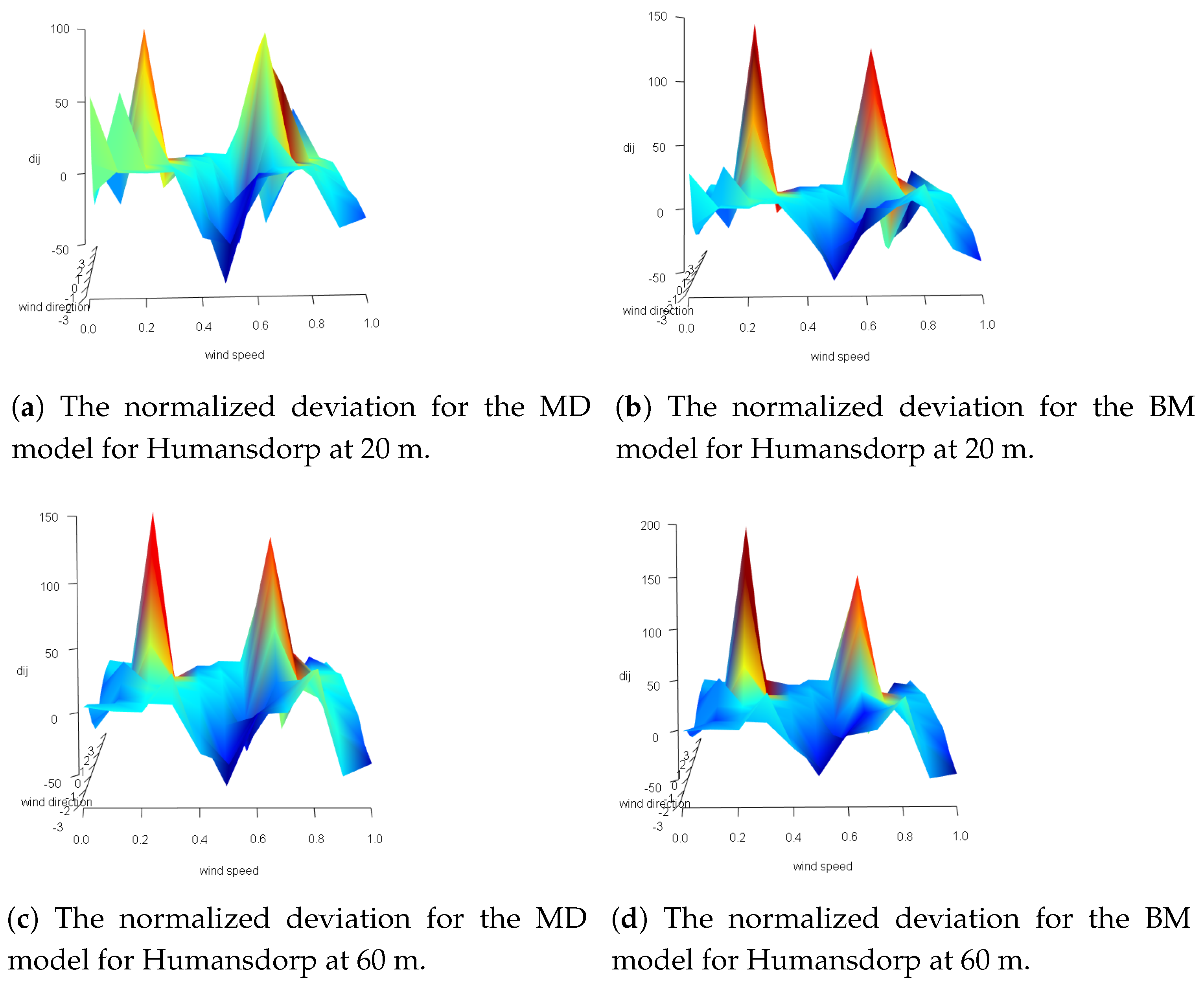
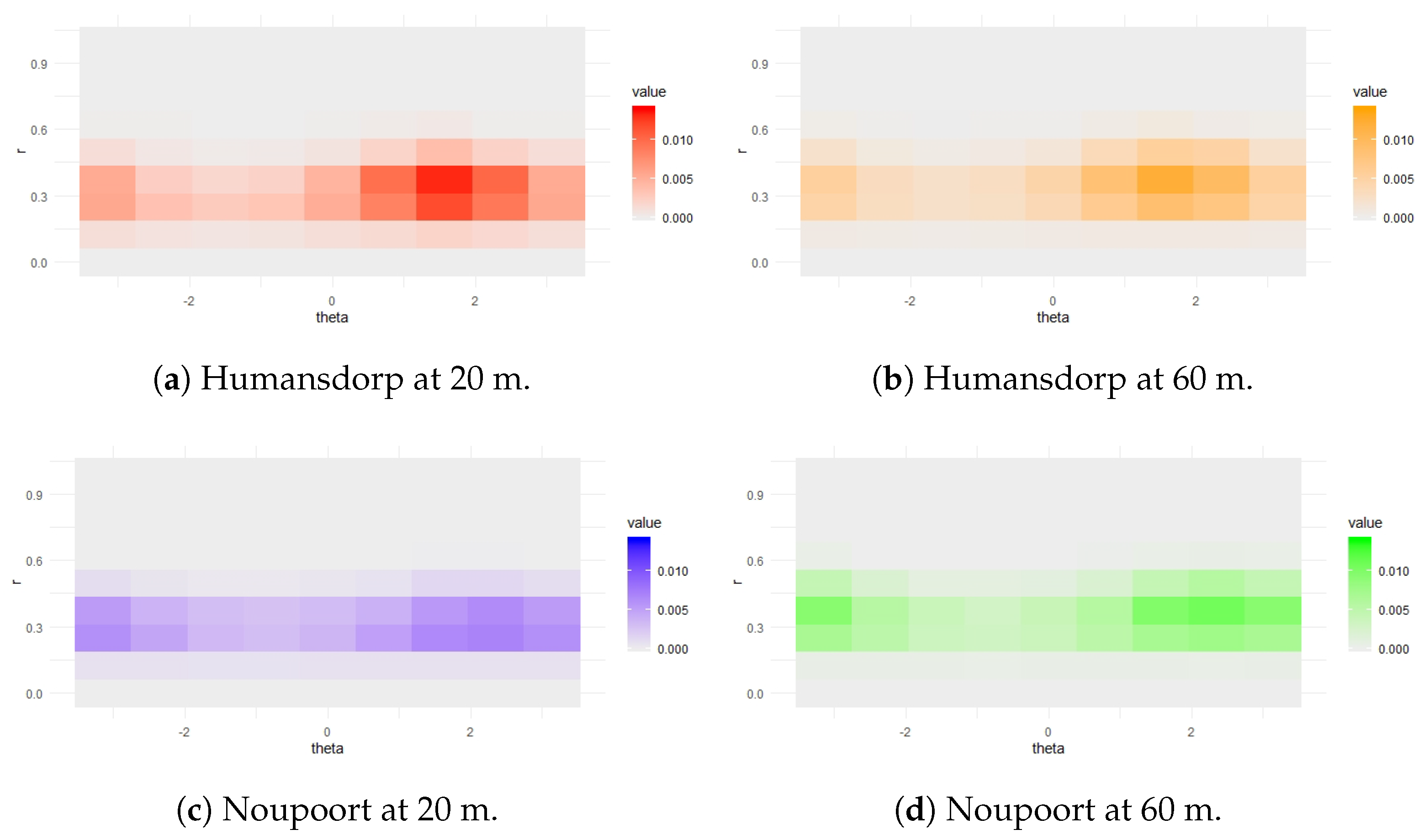
• For the Humansdorp location at 20 m, the SPM model performs the best overall. The BM model performs the best from the parametric models.
• For the Humansdorp location at 60 m, the SPM model performs the best overall. The MD model performs the best from the parametric models.
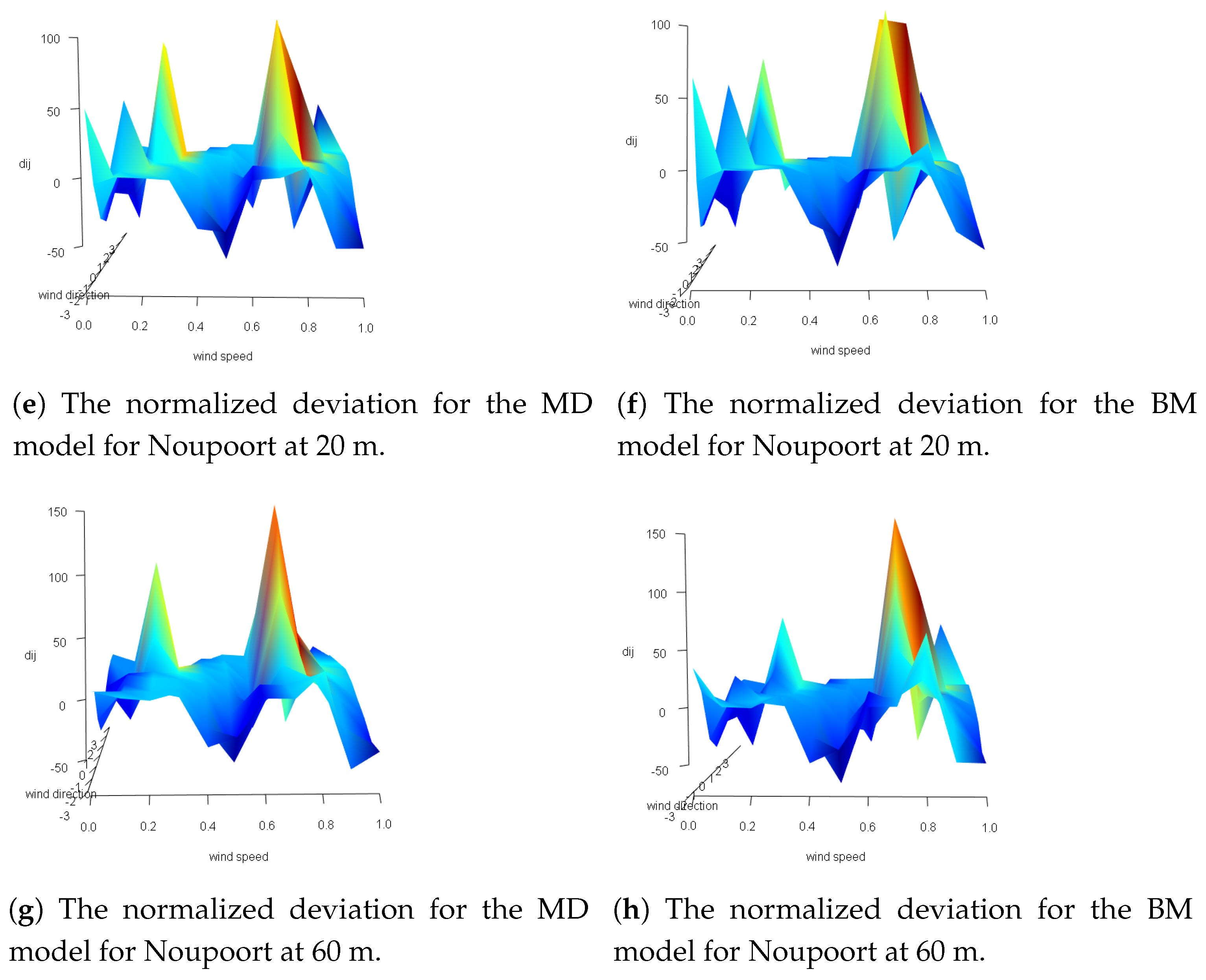
• For the Noupoort location at 20 m, the SPM model performs the best overall. The BM model performs the best from the parametric models.
• For the Noupoort location at 60 m, the SPM model performs the best overall. The BM model performs the best from the parametric models.
• The SPM model outperforms overall based on the performance measures. This model has the advantage of limited distributional assumptions. However, it is worth noting that the selection of the bandwidth plays an important role in statistical analysis.
• The BM model performs the best from the parametric models based on the performance measures. This is a result of the model’s flexibility in capturing bimodality and skewness present in the data. The presence of bimodality and skewness can be seen in the data plots (see Figure 2 and Figure 3).

For comparison purposes, it is important to note that, since our model is fitted using the maximum-likelihood method (for the parameters), we can use the AIC and/or BIC, which are based on the likelihood method. The squared error loss can be used to refine the aforementioned criteria measures as discussed in [33].

In

Table 10. Normalized deviations for parametric models for each location.

Station	Height (m)	Model	Median	Range
Humansdorp	20	MD	−0.2708471	(−86.41038; 114.30956)
Humansdorp	20	BM	−0.2757685	(−66.82174; 168.59107)
Humansdorp	60	MD	−0.3938287	(−73.57794; 154.53348)
Humansdorp	60	BM	−0.8428266	(−74.65866; 201.50158)
Noupoort	20	MD	−0.4002134	(−84.15884; 116.17518)
Noupoort	20	BM	−0.2386832	(−80.73554; 126.18355)
Noupoort	60	MD	−0.3757053	(−76.41617; 162.44165)
Noupoort	60	BM	−0.08373657	(−73.58869; 179.88564)

, a summary of the normalized deviations for the parametric models for each location is provided. Figure 4 illustrates the normalized deviation plots for the parametric models for each location. Using this metric from Table 10, we can conclude that the MD model has a better fit for the Humansdorp location and the BM model fits better for the Noupoort location, as the median of the normalized deviation is closer to zero.

For the wind power density, (1), we substitute the proposed parametric base models $f_{X,\mathsf{\Theta }}(x,\theta )$ (joint model of wind speed and wind direction) to evaluate the wind energy. Based on the parametric models of best fit in Table 9, the wind power density is plotted in Figure 5 for the estimated parameter values given in Table 9.

The intensity plots for the estimated wind power density (1) for when the base model is considered as the SPM model (model of best fit) are given in Figure 6 for various values of $\theta$ and x.

Figure 6 illustrates that the estimated wind power density is maximal when the wind is blowing in a North Westerly direction (for $\theta$ between $1.57$ to $2.36$, given that $-\pi$ is the North direction) and when the wind speed is low to moderate. It can also be noted that at the Humansdorp location a height of 20 m displays a stronger wind power density compared to the height of 60 m, and at the Noupoort location, a height of 60 m displays a stronger wind power density compared to the height of 20 m.

6. Conclusions

In this paper, we propose a class of joint probability models for the wind speed and wind direction data at Humansdorp and Noupoort. This class accounts for an embedded correlation structure between the wind speed and wind direction and additionally captures the skewness and bimodality present in the data. Based on the circular–linear correlation coefficient, the need to account for dependency between the wind speed and wind direction is emphasized. The wind energies at the two locations were evaluated using the SPM model (best performing model) to determine the wind energy potential at the different heights for the two locations. One of the reviewers pointed out that a comparisons between the models proposed in this paper and existing joint wind speed and wind direction models are inappropriate due to the differences in the definitions of the manifolds. Considering the situation surrounding the supply of electricity in South Africa, the need for investigating and investing in alternative renewable energy sources is of utmost importance to the socioeconomic development of the country.

References

1. Saidur, R.; Rahim, N.; Islam, M.; Solangi, K. Environmental impact of wind energy. Renew. Sustain. Energy Rev. 2011, 15, 2423–2430. [Google Scholar] [CrossRef]
2. Jung, C.; Schindler, D. Sensitivity analysis of the system of wind speed distributions. Energy Convers. Manag. 2018, 177, 376–384. [Google Scholar] [CrossRef]
3. Carta, J.; Ramirez, P.; Velazquez, S. A review of wind speed probability distributions used in wind energy analysis: Case studies in the Canary Islands. Renew. Sustain. Energy Rev. 2009, 13, 933–955. [Google Scholar] [CrossRef]
4. Soukissian, T.H.; Karathanasi, F.E. On the selection of bivariate parametric models for wind data. Appl. Energy 2017, 188, 280–304. [Google Scholar] [CrossRef]
5. Porté-Agel, F.; Wu, Y.T.; Chen, C.H. A numerical study of the effects of wind direction on turbine wakes and power losses in a large wind farm. Energies 2013, 6, 5297–5313. [Google Scholar] [CrossRef]
6. Herbert-Acero, J.; Probst, O.; Réthoré, P.E.; Larsen, G.; Castillo-Villar, K. A review of methodological approaches for the design and optimization of wind farms. Energies 2014, 7, 6930–7016. [Google Scholar] [CrossRef]
7. Waewsak, J.; Chaichana, T.; Chancham, C.; Landry, M.; Gagnonc, Y. Micro-siting wind resource assessment and near Shore wind farm analysis in Pakpanang district, Nakhon Si Thammarat province, Thailand. Energy Procedia 2014, 52, 204–215. [Google Scholar] [CrossRef] [Green Version]
8. Zhang, M.H. Wind Resource Assessment and Micro-Siting: Science and Engineering; John Wiley & Sons: Hoboken, NJ, USA, 2015. [Google Scholar]
9. Song, M.; Chen, K.; Zhang, X.; Wang, J. Optimization of wind turbine micro-siting for reducing the sensitivity of power generation to wind direction. Renew. Energy 2016, 85, 57–65. [Google Scholar] [CrossRef]
10. Carta, J.A.; Ramirez, P.; Bueno, C. A joint probability density function of wind speed and direction for wind energy analysis. Energy Convers. Manag. 2008, 49, 1309–1320. [Google Scholar] [CrossRef]
11. Han, Q.; Hao, Z.; Hu, T.; Chu, F. Non-parametric models for joint probabilistic distributions of wind speed and direction data. Renew. Energy 2018, 126, 1032–1042. [Google Scholar] [CrossRef] [Green Version]
12. Feng, J.; Shen, W. Modelling wind for wind farm layout optimization using joint distribution of wind speed and wind direction. Energies 2015, 8, 3075–3092. [Google Scholar] [CrossRef] [Green Version]
13. Sanusi, N.; Zaharim, A.; Mat, S.; Sopian, K. Comparison of Univariate and Bivariate Parametric Model for Wind Energy Analysis. J. Adv. Res. Fluid Mech. Therm. Sci. 2018, 49, 1–10. [Google Scholar]
14. Gugliani, G.; Sarkar, A.; Ley, C.; Mandal, S. New methods to assess wind resources in terms of wind speed, load, power and direction. Renew. Energy 2018, 129, 168–182. [Google Scholar] [CrossRef]
15. Zhang, J.; Chowdhury, S.; Messac, A.; Castillo, L. A multivariate and multimodal wind distribution model. Renew. Energy 2013, 51, 436–447. [Google Scholar] [CrossRef]
16. Ley, C.; Verdebout, T. Modern Directional Statistics; CRC Press: Boca Raton, FL, USA, 2017. [Google Scholar]
17. Johnson, R.A.; Wehrly, T. Measures and models for angular correlation and angular–linear correlation. J. R. Stat. Soc. Ser. B (Methodol.) 1977, 39, 222–229. [Google Scholar] [CrossRef] [Green Version]
18. Zhang, L.; Li, Q.; Guo, Y.; Yang, Z.; Zhang, L. An investigation of wind direction and speed in a featured wind farm using joint probability distribution methods. Sustainability 2018, 10, 4338. [Google Scholar] [CrossRef] [Green Version]
19. Basile, S.; Burlon, R.; Morales, F. Joint probability distributions for wind speed and direction. A case study in Sicily. In Proceedings of the 2015 International Conference on Renewable Energy Research and Applications (ICRERA), Palermo, Italy, 22–25 November 2015; pp. 1591–1596. [Google Scholar]
20. Erdem, E.; Shi, J. Comparison of bivariate distribution construction approaches for analysing wind speed and direction data. Wind Energy 2011, 14, 27–41. [Google Scholar] [CrossRef]
21. Hennessey, J.P., Jr. A comparison of the Weibull and Rayleigh distributions for estimating wind power potential. Wind Eng. 1978, 2, 156–164. [Google Scholar]
22. Mardia, K.V.; Jupp, P.E. Directional Statistics; John Wiley & Sons: Hoboken, NJ, USA, 2009; Volume 494. [Google Scholar]
23. Bekker, A.; Nagar, P.; Arashi, M.; Rautenbach, H. From Symmetry to Asymmetry on the Disc Manifold: Modeling of Marion Island Data. Symmetry 2019, 11, 1030. [Google Scholar] [CrossRef] [Green Version]
24. Burnham, K.P.; Anderson, D.R. A practical information-theoretic approach. Model Selection and Multimodel Inference, 2nd ed.; Springer: New York, NY, USA, 2002. [Google Scholar]
25. Fabozzi, F.J.; Focardi, S.M.; Rachev, S.T.; Arshanapalli, B.G. The Basics of Financial Econometrics: Tools, Concepts, and Asset Management Applications; John Wiley & Sons: Hoboken, NJ, USA, 2014. [Google Scholar]
26. Wagenmakers, E.J.; Ratcliff, R.; Gomez, P.; Iverson, G.J. Assessing model mimicry using the parametric bootstrap. J. Math. Psychol. 2004, 48, 28–50. [Google Scholar] [CrossRef]
27. Claeskens, G.; Carroll, R.J. An asymptotic theory for model selection inference in general semiparametric problems. Biometrika 2007, 94, 249–265. [Google Scholar] [CrossRef]
28. Murphy, S.A.; Van der Vaart, A.W. On profile likelihood. J. Am. Stat. Assoc. 2000, 95, 449–465. [Google Scholar] [CrossRef]
29. Xu, R.; Vaida, F.; Harrington, D.P. Using profile likelihood for semiparametric model selection with application to proportional hazards mixed models. Stat. Sin. 2009, 19, 819. [Google Scholar] [PubMed]
30. Fu, Y.Z.; Chen, X.D. Model selection of generalized partially linear models with missing covariates. J. Stat. Plan. Inference 2012, 142, 126–138. [Google Scholar] [CrossRef]
31. Zhang, X.; Liang, H. Focused information criterion and model averaging for generalized additive partial linear models. Ann. Stat. 2011, 39, 174–200. [Google Scholar] [CrossRef] [Green Version]
32. Buttarazzi, D.; Pandolfo, G.; Porzio, G.C. A boxplot for circular data. Biometrics 2018, 74, 1492–1501. [Google Scholar] [CrossRef]
33. Ullah, A.; Wang, H. Parametric and nonparametric frequentist model selection and model averaging. Econometrics 2013, 1, 157–179. [Google Scholar] [CrossRef] [Green Version]
Figure 1. Locations of the two stations in South Africa (Google Maps, 2020. Google Maps (online). Available through: <https://www.google.com/maps> (Accessed 05 March 2020)).
Sustainability 12 04371 g001
Figure 2. Data plots for the Humansdorp location.
Sustainability 12 04371 g002aSustainability 12 04371 g002b
Figure 3. Data plots for the Noupoort location.
Sustainability 12 04371 g003aSustainability 12 04371 g003b
Figure 4. (ad) Plots of the normalized deviations for the parametric models for the Humansdorp location. (eh) Plots of the normalized deviations for the parametric models for the Noupoort location.
Sustainability 12 04371 g004aSustainability 12 04371 g004b
Figure 5. Plots and contour plots of the estimated wind power density (1) for each location with the parametric model of best fit as the base joint model of wind speed and wind direction.
Sustainability 12 04371 g005
Figure 6. Estimated intensity plots of wind power density (1) values of the semi-parametric model for various values of x and θ .
Sustainability 12 04371 g006