1. Introduction
The plan to build up the Xiong’an new area was announced by the Chinese Central Government on 1 April 2017. The long-term goal is to build a modernized and environmentally friendly urban area to largely undertake non-essential functions of Beijing as the capital city in China. Due to its strategic and economic importance, the Chinese Central Government has implemented high standard on its buildup. Thus, monitoring urban dynamic in the Xiong’an new area is necessary and valuable in terms of its sustainable development.
High-Rising Buildings (HRBs) are a typical artificial land cover and mainly serve as high-end commercial and business centers and residential apartments. With their unique characteristics and functions, HRBs have a great impact on urban environment and socioeconomics. For example, HRBs influence local climate in urban areas by modifying energy balance and roughness of the urban surface, which are closely related to urban heat island effect [
1,
2]; HRBs have obvious advantages at improving the efficiency of resources and energy; HRBs always contain a very high intensity of population and make people easily vulnerable to contagious diseases and other disasters. Therefore, the speed and amount of the increase of HRBs in urban areas can be a useful indicator of urban development.
Although HRBs are quite visually distinct for their large height in urban areas, no consistent and clear definition has ever been given to HRBs in the context of the large-scale monitoring of HRBs. Here, we consider HRBs as spatial clusters of buildings and each cluster represents spatially connected buildings with relatively uniform height. The threshold of the height works as the only parameter in defining HRBs. In the north China plain, and even most of residential areas in China, traditional buildings have no more than six floors. Typically, a building with six floors has a height of about 16 m. With the rapid urbanization in the last few decades, many buildings were constructed with more than six floors. Most of those newly constructed buildings include at least 10 floors and have a height of above 25 m. Based on these facts, we consider HRBs as building clusters with the average height of above 25 m.
Due to being effective and cost-efficient, remote sensing has been widely studied to monitor urban dynamic at various temporal and spatial scales [
3,
4,
5]. However, the study of HRBs is far behind that of other typical urban land covers such as vegetation and impervious surfaces in the remote sensing community. Complex 3D geometry and surface materials make large-scale monitoring HRBs, in a routine way, nearly impossible due to the lack of proper remote sensing data and efficient extraction methods. Recent Sentinel-2 data from the European Space Agency (ESA) open a new window to routinely monitor HRBs in large areas with its nadir viewing, 10 m spatial resolution, global coverage, short revisiting interval, and opening access policy, and so on [
6]. Almost in parallel with the availability of Sentinel-2 data, the emergence of deep learning models largely transforms the way of information extraction from remote sensing data [
7,
8]. Among the models, Fully Convolutional Networks (FCN) [
9,
10], initially proposed to conduct sematic segmentation on natural images, can be well used for the pixel-wise classification of remote sensing data. Our previous work successfully developed an FCN-based method to extract HRBs from Sentinel-2 images [
11]. Above 95 percent of overall accuracy measured by F1 score is obtained in the core of Xiong’an new area by the FCN-based method, which is much better than that of traditional supervised classification methods.
This paper extends our previous work on HRB detection in single images and aims to detect and analyze the increase of HRBs in 39 counties located in the center of the Xiong’an new area within a two-year period started from 2017. Our main contributions are twofold. We develop a novel FCN based method to detect the increase of HRBs from multi-temporal Sentinel-2 data in large areas. Additionally, we provide an analysis of the increased HRBs in 39 counties in terms of their quantities, spatial distribution and driving forces at the county level.
2. Materials and Methods
2.1. Study Region and Data
Our study region is located in the center of the Xiong’an new area. It covers 39 counties in Hebei province and has a total area of about 26,000 km
2. To detect the increase of HRBs between 2017 and 2019, a total of 10 images from 4 tiles of Sentinel-2 data were selected. As HRBs were mainly discriminated based on the spatial structure, only three 10 m RGB bands of each Sentinel-2 data were used in the study. Further considering the availability of cloud free data and the seasonal dynamic features of HRBs in optical remote sensing images, and also more visually distinctive features of HRBs with long shadows in the winter and early spring in the study area, Sentinel-2 data acquired in the later winter and early spring were selected. The Sentinel-2 images used in our study are shown in the
Table 1. The study region and related data are illustrated in
Figure 1.
To validate our HRB change detection method, HRB samples were manually extracted from 1 m or less spatial resolution images from the Google Earth. The feasibility of the manual interpretation of HRBs is due to the fact that the height of buildings is not evenly distributed in urban areas, and also HRBs can be visually discriminated by their unique spatial structures. To analyze the increased HRBs in 39 counties in terms of their quantities, spatial distribution and driving forces at the county level, we selected five factors at the county level that closely related to the increase of HRBs including the volume of Gross Domestic Product (GDP) and the Number of Permanent Residents (NPR) in 2016, transportation accessibility, the terrain in the county, and policy in urban development as explained in
Table 2. We graded each factor into different levels based on various kinds of statistics at county level and expert knowledge as listed in the
Table 3.
2.2. FCN Based HRBs Extraction Method
This study uses a ready-to-use FCN model that was successfully developed in our previous work to extract HRBs from 10 m Sentinel-2 images in the Xiong’an new area. Above 95 percent of overall accuracy measured by F1 score can be achieved [
11]. The workflow is illustrated at the top of
Figure 2.
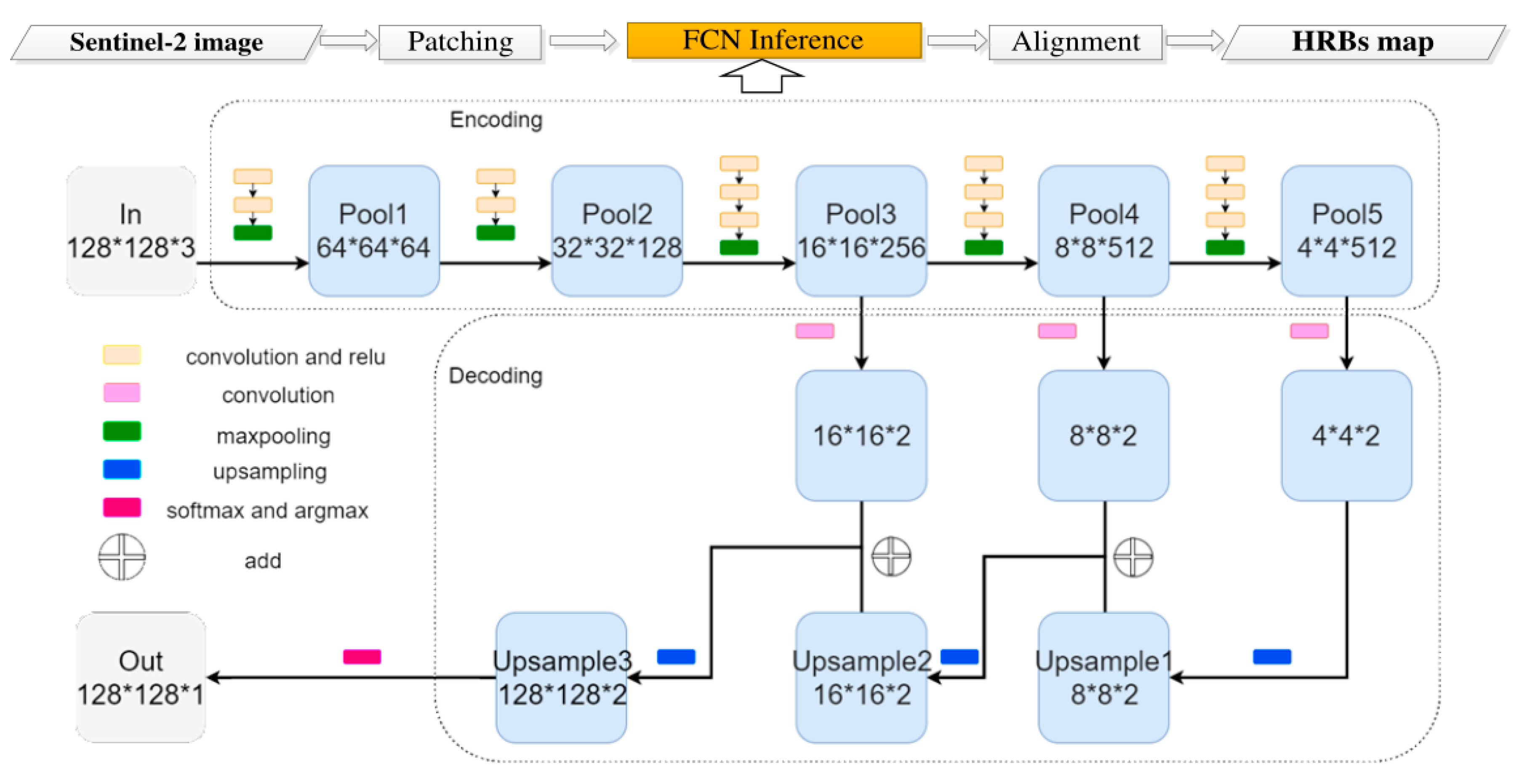
For the procedure of the FCN based method, each input image is firstly clipped into patches with the size of 1024 × 1024 in this study. The clipped patches are processed by a trained FCN model as shown at the bottom of
Figure 2. The inference results are spatially aligned accordingly. The final output is a binary image of HRBs with the same size of the input image. Here, the patch size for inference can be much larger than the patch size used in the training. This is because the FCN inference works in a parallel mode and each location is only affected by its effective receptive field which has a size of 32 × 32 pixels in our model. Additionally, we set the step of the moving window in the patch clip to 32 pixels to alleviate negative effect caused by spatial alignment of the boundary in the final result.
The architecture of the FCN model includes an encoder and a decoder. In the encoder, VGG-16 model [
12] is employed to encode each input patch into small but informative features. The encoded features are then fed into the decoder to hierarchically recover spatial contexts of the label. The dimension of features in each decoded layer is equal to the number of classes (two in our case, HRBs and others). The upsampling in the decoder is performed based on a transposed convolution with a fixed filter defined by the bilinear interpolation. Two skip layers are added to enhance the spatial detail of label recovery. In the output layer, the softmax function transforms the decoded features into probabilities of HRBs and others, and then argmax selects the label with the highest probability for each location and obtains a pixel-wise map of HRB mask. The FCN model was trained by the Adam method with a decaying learning rate. A similar model was used in the extraction of the fine water body from sub-meter spatial resolution optical images in our previous work [
13].
2.3. The Flowchart of Detecting and Analyzing the Increase of HRBs in Our Study
In our study, HRBs were firstly extracted from Sentinel-2 images in 2017 and 2019 respectively based on the FCN model, and then the increases of HRBs between 2017 and 2019 were detected through a novel object-oriented change detection procedure. Furthermore, the detected increases of HRBs were validated on their accuracy and then they were analyzed in terms of quantities, spatial distribution and driving forces at the county level. The flowchart of our study can be divided into 7 steps as follows.
- (1)
Mosaic images in 2017 and extract HRBs from mosaicked images based on the trained FCN model. A similar procedure was conducted on images in 2019.
- (2)
Clip the detected HRBs based on the outer boundary of the study region, and vectorize the clipped HRBs detection results into polygons in 2017 and 2019 respectively.
- (3)
Slightly refine the FCN derived HRBs polygons by manually editing a small amount of omitted HRBs and removing a few shadows in mountainous areas and small water bodies which are quite similar to HRBs in the images. This step is necessary due to the change detection being very sensitive to detection results.
- (4)
Change detection of HRBs was conducted by removing the intersection of detected HRB in 2017 and 2019 from the detected HRBs in 2019. Here, we only consider increase of HRBs because the decrease of HRBs within a two-year period in urban areas is very rare in reality.
- (5)
Small and thin regions in the change map were removed by employing two criteria: the ratio of area and length of long axis is less than 14, and total area is less than 4000 m2. The thresholds were empirically set based on expert interpretation of the detected results.
- (6)
The accuracy of the detected increased HRBs in polygons was validated by using manually interpreted samples from typical areas in the study region.
- (7)
The validated increases of HRBs were analyzed in terms of their quantities, spatial distribution and driving forces at the county level. To analyze the driving forces, permutation importance based on the Random Forest model [
14] was used to measure the significance of five selected factors regarding to the increase of HRBs.
3. Results and Analysis
3.1. Validation of Detection Results of the Increased HRBs
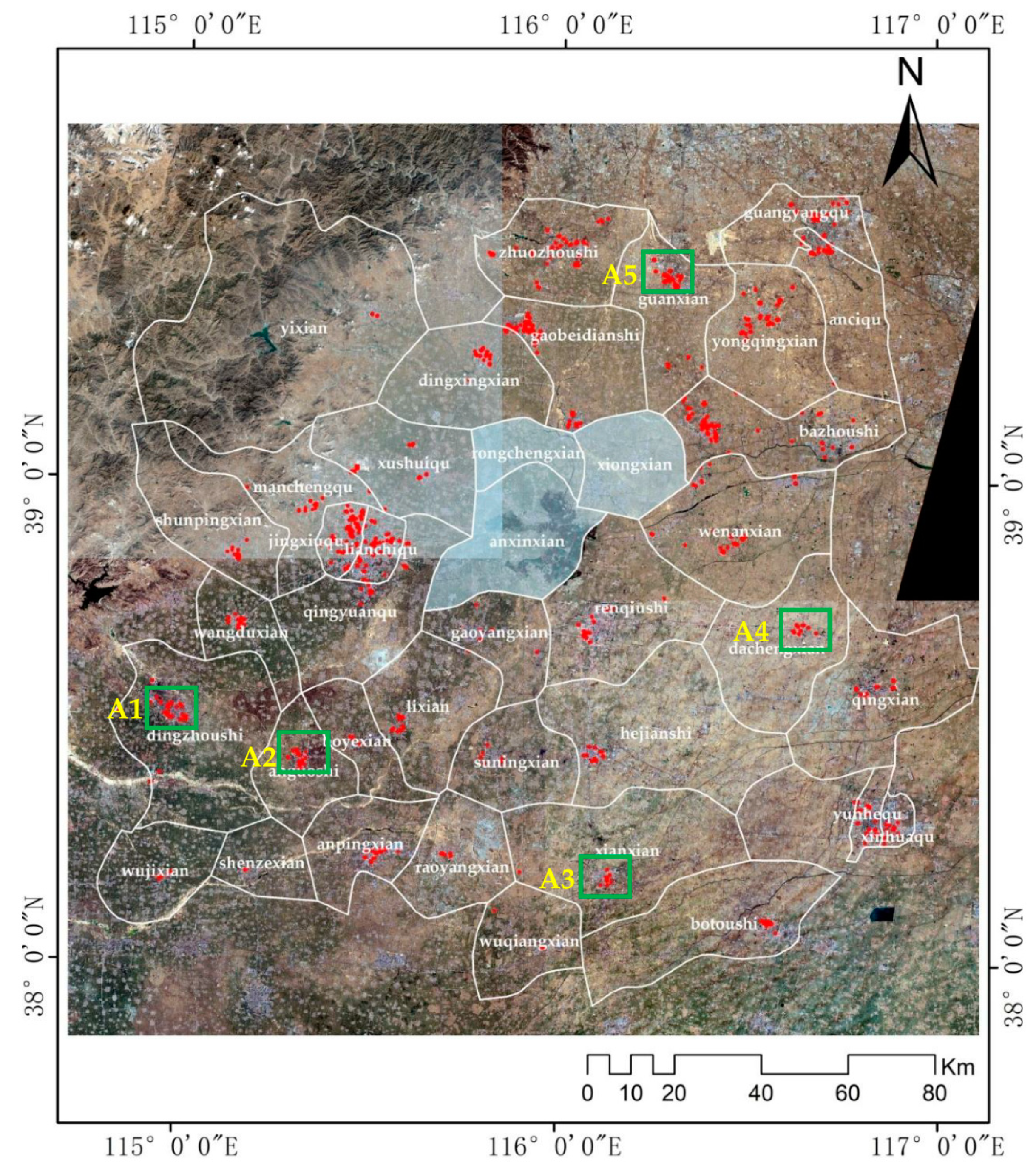
Figure 3 illustrates the detection results of the increased HRBs. Five typical areas were selected in the study region to quantitatively validate the results. For each validation area, the ground truths of changes were manually interpreted from Google Earth images with a similar imaging date as the corresponding Sentinel-2 images. The block number of HRBs is used as the basic element in the validation for its simplicity in counting. Each block is a polygon which is the boundary of a spatially connected cluster of HRBs. We use the Intersection-Over-Union (IOU) as the criteria to evaluate each block. We consider a detected block as correct if the value of IOU between the block in the detection and the corresponding block in the ground truth is higher than 80 percent.
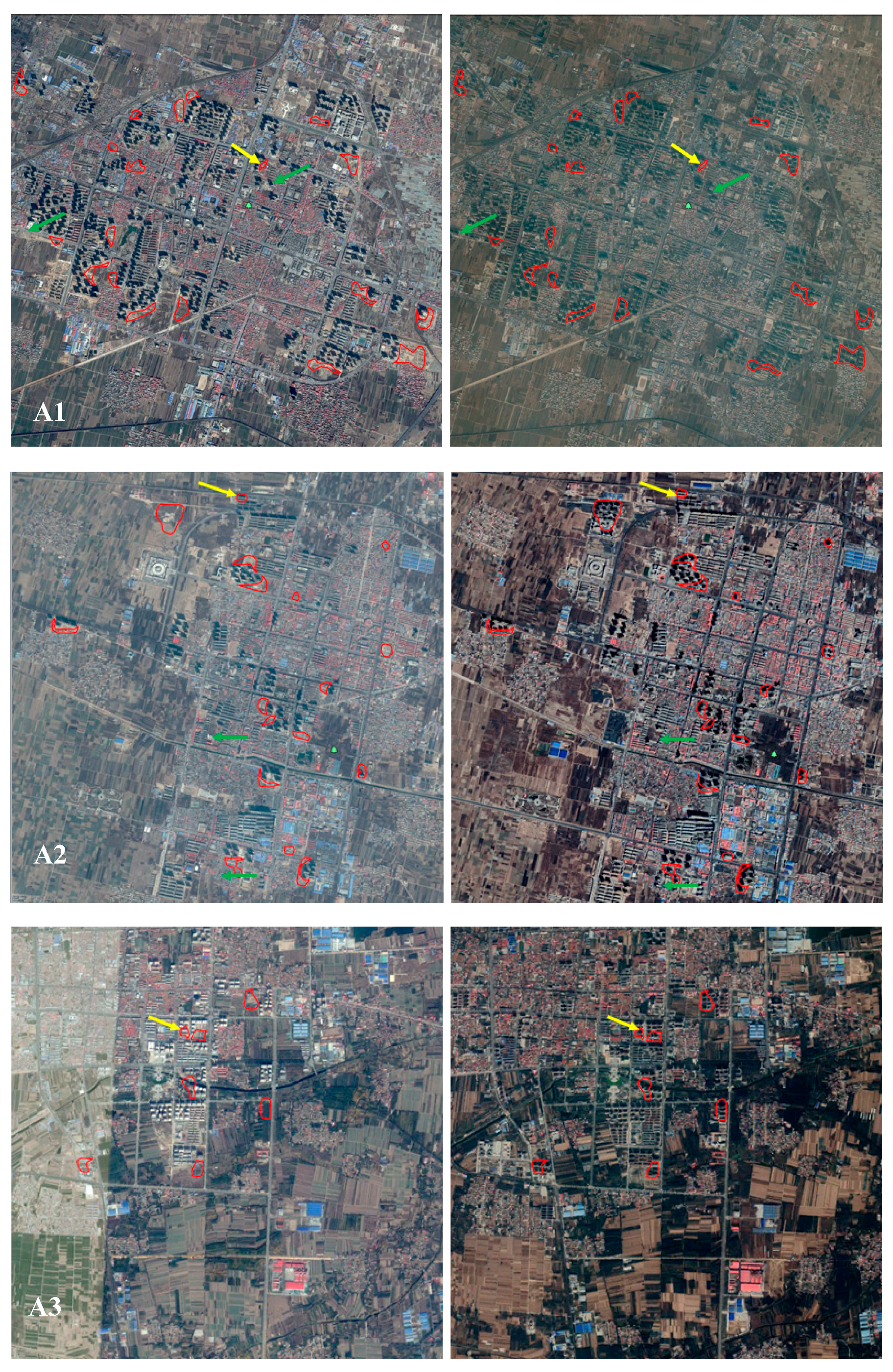
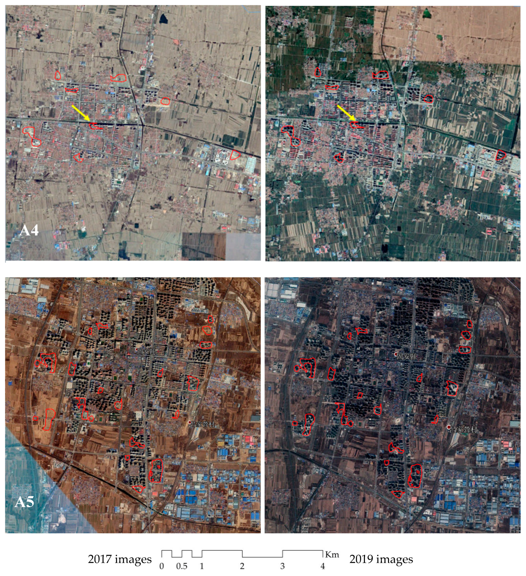
Table 4 shows validation results of all five areas. We achieve an average overall accuracy of 95.87% with a False Alarm of 8.25%. The accuracy for different areas varies slightly. It is clear that nearly all errors, either omission or commission, are HRBs with relatively small areas. For qualitative validation purposes, we illustrate all five validation results of each area in
Figure 4.
3.2. Analysis of Increased HRBs at the County Level
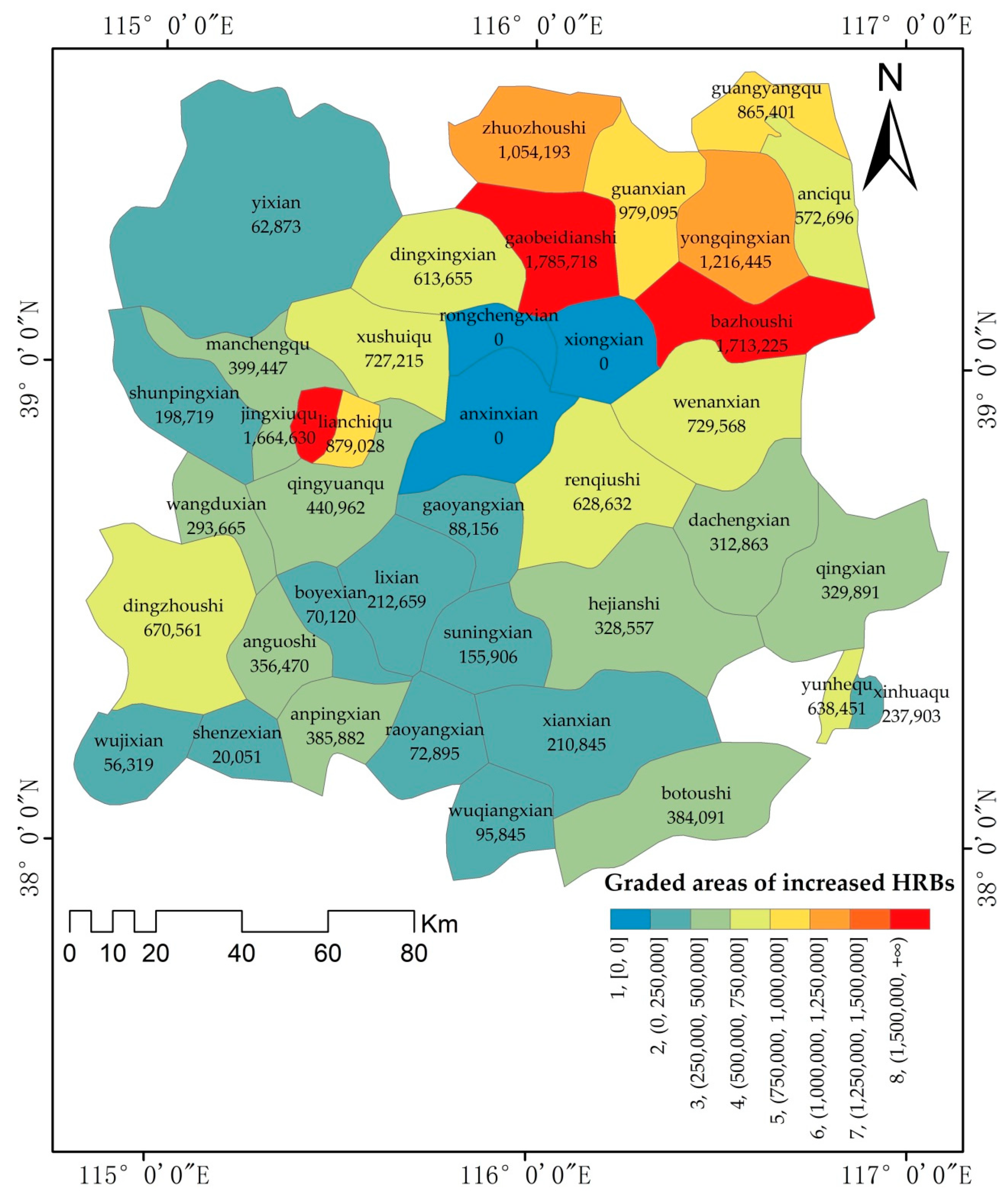
Figure 5 shows the maps of the area of increased HRBs at the county level. It is clear that the increase of HRBs between 2017 and 2019 varies a lot among counties. The dynamic range of the area changes from zero to about 1.78 million m
2. The most distinct increase is located in the north-east of the study area which neighbors the capital city of China, Beijing. The secondary obvious increase is located in the city of Baoding which is one of the largest cities in Hebei province. The increase of HRBs in the three core counties of Xiong’an new area is zero. Meanwhile, as it is shown in
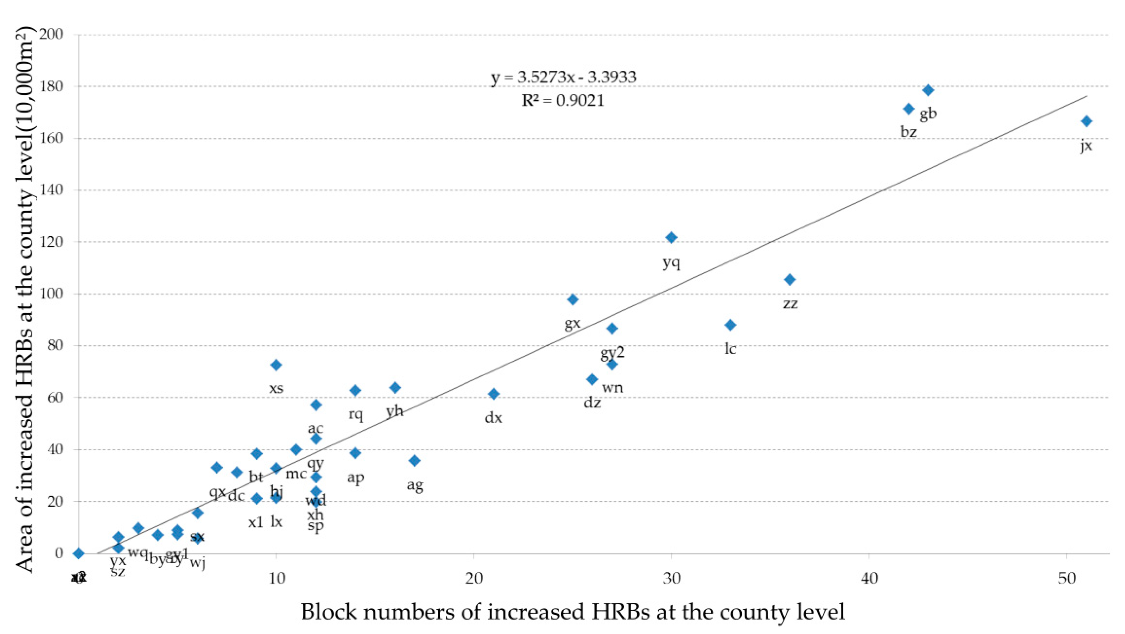
Figure 6, the linear correlation coefficient is around 0.90 between the area and the block number at the county level, indicating that the spatial distribution of the area and the block number of the increased HRBs at the county level varies a little.
To understand the driving forces of the increase of HRBs, we trained a Random Forest model with the selected five factors in
Table 3 as independent variables and the increase of HRBs as dependent variable. According to the inference result of the trained Random Forest model, the increase of HRBs can be predicted by the five factors with above 90% overall accuracy. Furthermore, permutation importance based on the Random Forest model is derived to evaluate the significance of the factors. The permutation importance is defined to be the decrease in a model score when a single feature value is randomly shuffled [
14]. The only parameter of the model is the number of repetitions for the feature shuffling, and it was set to 10 in our experiment. The permutation importance of five selected factors is shown in
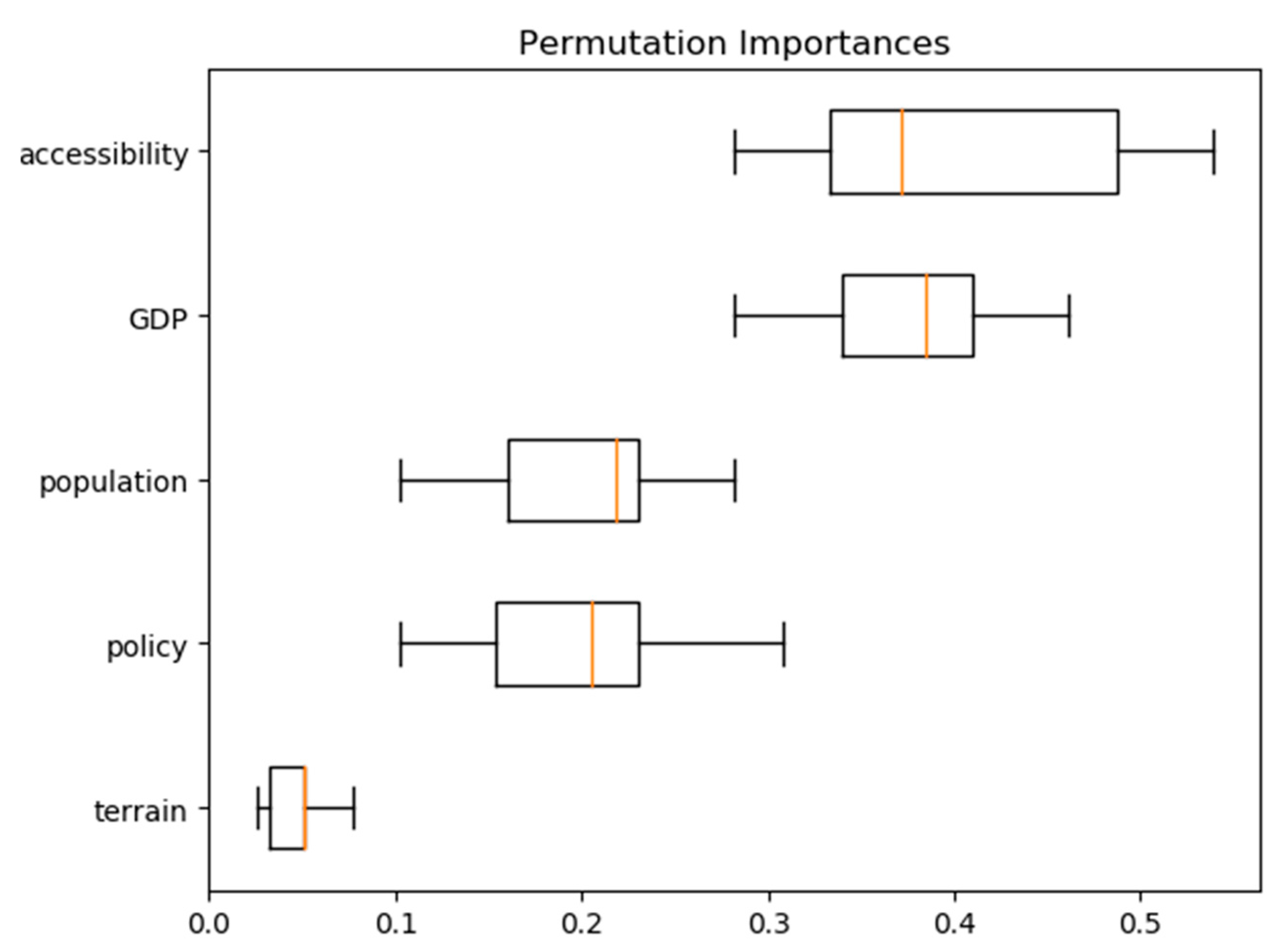
Figure 7. It can be seen that, although the prediction accuracy is relatively high in the inference, no single factor can fully explain the increase of HRBs. Among the five selected factors, GDP and transportation accessibility have clearly higher impacts than the other three; NPR and policy follow as the secondary group; the terrain has the lowest influence on the increase.
4. Discussion
The increase in HRBs is investigated to monitor the dynamic of urban development in the center of the Xiong’an new area. HRBs are quite different from the commonly-used impervious area in terms of function and physical characteristics. For obvious reasons of simplicity and consistency, the impervious area has been widely studied in the remote sensing community [
15,
16,
17,
18,
19]. Due to benefits from the availability of large amount of satellite images (e.g., Landsat, SPOT and GaoFen) and the advancement of the cloud computing infrastructure (e.g., Google Earth Engine [
20]) in last decade, a number of multi-temporal impervious maps at local and even global scales have been developed [
18,
19]. However, due to the complexity of the urban area in terms of its physical and functional properties, impervious area has its limitation at fully characterizing the urban area. To better understand the urban process, dynamic monitoring detailed land cover and land use in urban areas becomes increasingly important [
21,
22]. Our definition of HRBs is closely related to the high-rising buildings defined in the Local Climate Zones (LCZs) [
2]. Our definition can be largely considered to be the combination of LCZ1 and LCZ4. These two types share a similar height property of above 25 m, while they are treated separately in the LCZs for their difference in spatial density of buildings which is relevant to urban climate study.
The change detection procedure proposed in this paper was a natural extension of our previous HRB detection method [
11]. In the procedure, we adopt a heuristic objected-oriented change detection strategy. The strategy is selected mainly based on two distinct characteristics of HRBs in 10 m Sentinel-2 images. First and foremost, HRBs have their geometric structures largely kept in the image with the spatial resolution of 10 m; another is that the boundary of HRBs in the 10 m image varies with many factors such as spatial configuration and viewing geometry. Both of the two characteristics make the pixel-based and/or direct change detection strategy inefficient, if not impossible [
23,
24]. Our method can be extended to large scale areas because of the robust FCN method and the redundant and freely accessible Sentinel-2 images. The FCN method is robust in feature learning and the detection of HRBs once enough training samples are provided. Meanwhile, 10 m Sentinel-2 data provide valuable and economical resources to routinely monitor urban area in a new and fine-grained perspective compared to commonly used Landsat data.
The choice of IOU as the accuracy measurement is due to the fact that IOU works in an object-oriented way and fits well to situations when the size of interested target is relatively larger than pixel size. Our proposed procedure cannot guarantee an accuracy of 100 percent, though we introduce a manual process mainly conducted on Sentinel-2 data alone, as indicated in step 3 of our flowchart, to improve the detection result. Due to the complex 3D geometric structures and artificial materials in urban areas, the image features of HRBs in 10 m Sentinel-2 data vary a lot with the imaging date and geometry, and it is almost impossible that a block of HRBs extracted from one image would perfectly match with the block of the same HRBs in a different image, especially when the spatial resolution of two images differs a lot.
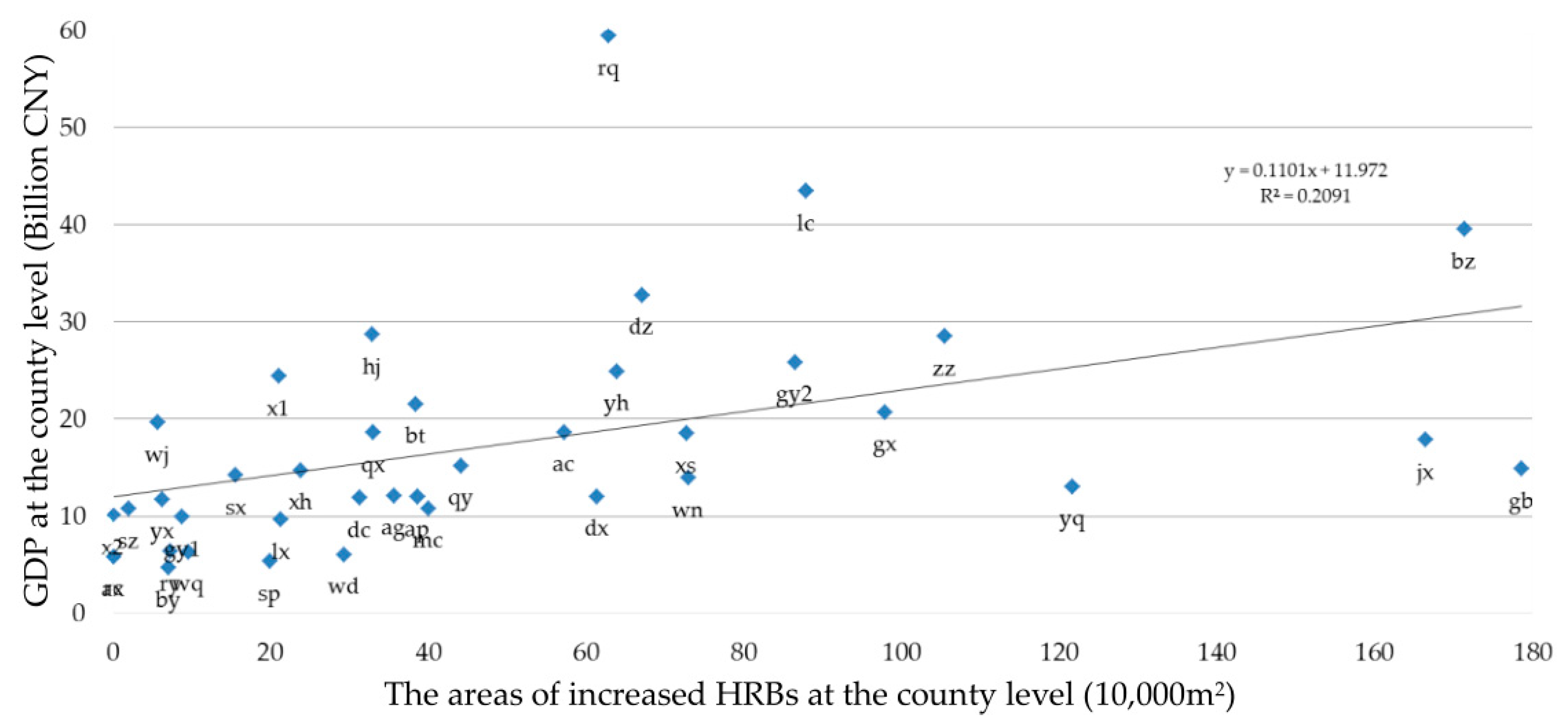
Our results show that no single selected factor can explain the pattern of the increase of HRBs in 39 counties well. However, the relatively high importance of GDP and transportation accessibility is consistent with common senses. High GDP generally implies that the local government has more money to be put into urban infrastructure construction. We can see a weak positive linear correlation between GDP and the increase of HRBs, as shown in
Figure 8. Good transportation accessibility enhances the attractiveness of the county in terms of its living environment. This is well indicated by counties in the peripheral regions of Beijing and Baoding. A unique factor is the policy in the study region. The central government issued different levels of restriction over urban construction in the Xiong’an new area since 2017. The zero increase of HRBs in the three core counties demonstrates the effect of the policy in an extreme way. However, there are still a few exceptions, such as Renqiushi, whose economy largely relies on the petroleum industry and agriculture, both of which do not contribute to the increase of HRBs. A similar reason can be attributed to NPR in counties that are fulfilled by a large amount of people living in rural areas. Thus, there are still spaces to introduce additional factors to obtain a detailed explanation about the increase of HRBs in each county.
5. Conclusions
Aiming at monitoring the urban dynamic of the Xiong’an new area, this paper proposed a procedure to detect and analyze the increase of HRBs between 2017 and 2019 in 39 counties in the center of the Xiong’an new area. Sentinel-2 images with 10 m spatial resolution acquired in 2017 and 2019 were used in our study. A novel change detection strategy based on Fully Convolutional Networks was developed to extract the increase of HRBs. The detected increases were validated and further analyzed in terms of their quantities, spatial distribution and driving forces at the county level. The results indicate that our method can effectively detect the increase of HRBs in large urban areas. The spatial distribution of the increased HRBs varies a lot in the 39 counties. Counties in the north-east and the mid-west of the study region account for most of the increase. GDP and accessibility contribute most to the increase. The impact of policy is distinctive, especially in the three core counties. The terrain seems to be not closely related to the increase of HRBs at the county level as other factors do, though terrain is an important factor to be seriously considered in the buildup of urban areas.
Our future study will focus on large-scale and long-term HRB detection and analysis. Due to the large diversity of image features of HRBs in different landscapes and imaging conditions, more training samples of HRBs may need to be collected and the parameters in the change detection may need to be refined. Meanwhile, we will improve the measurement of transportation accessibility by using more sophisticate models [
25] and also introduce more factors to further understand the pattern of the increase of HRBs in different counties. It is expected that there will be a stronger statistical correlation between long-term increases of HRBs and statistics of key social and economic factors at the county level. Finally, when being integrated into urban ecological [
26] or climate [
27] models, the long-term and large-scale information of HRBs can be more useful in real applications, such as environmental protection and urban planning, and become more valuable to support the sustainability of the Xiong’an new area and beyond.
Author Contributions
B.Z. and L.L. had the original idea for the study, with L.L. carried out the design. J.Z. and G.C. were responsible for programming and data processing. L.L. and L.G. conceived the experiments and carried out the analysis with assistant from Z.J., L.L. structured and drafted the manuscript. All authors have read and agreed to the published version of the manuscript.
Funding
This research was funded by National Natural Science Foundation of China (grant number 41971327), National Key Research and Development Program of China from MOST (grant number 2016YFB0501501) and the Strategic Priority Research Program of the Chinese Academy of Sciences (grant number XDA19080304).
Acknowledgments
We thank Zhi Yan for his work on the FCN model development during his stay as a visiting graduate student in RADI, CAS. Also Liwei Li thanks Wenzhi Liao from Ghent University, Belgium for the meaningful discussion on HRBs in early 2019 in Beijing.
Conflicts of Interest
The authors declare no conflict of interest.
References
- Bechtel, B.; Alexander, P.; Böhner, J.; Ching, J.; Conrad, O.; Feddema, J.; Mills, G.; See, L.; Stewart, I.D. Mapping Local Climate Zones for a Worldwide Database of the Form and Function of Cities. ISPRS Int. J. Geo Inf. 2015, 4, 199–219. [Google Scholar] [CrossRef]
- Stewart, I.D.; Oke, T.R. Local Climate Zones for Urban Temperature Studies. Bull. Am. Meteorol. Soc. 2012, 93, 1879–1900. [Google Scholar] [CrossRef]
- Miller, R.B.; Small, C. Cities from space: Potential applications of remote sensing in urban environmental research and policy. Environ. Sci. Policy 2003, 6, 129–137. [Google Scholar] [CrossRef]
- Esch, T.; Heldens, W.; Hirner, A.; Keil, M.; Marconcini, M.; Roth, A.; Zeidler, J.; Dech, S.; Strano, E. Breaking new ground in mapping human settlements from space—The Global Urban Footprint. ISPRS J. Photogramm. Remote Sens. 2017, 134, 30–42. [Google Scholar] [CrossRef]
- Taubenbock, H.; Esch, T.; Felbier, A.; Wiesner, M.; Roth, A.; Dech, S. Monitoring urbanization in mega cities from space. Remote Sens. Environ. 2012, 117, 162–176. [Google Scholar] [CrossRef]
- Li, J.; Roy, D.P. A Global Analysis of Sentinel-2A, Sentinel-2B and Landsat-8 Data Revisit Intervals and Implications for Terrestrial Monitoring. Remote Sens. 2017, 9, 902. [Google Scholar] [CrossRef]
- Zhang, L.; Zhang, L.; Du, B. Deep Learning for Remote Sensing Data: A Technical Tutorial on the State of the Art. IEEE Geosci. Remote Sens. Mag. 2016, 4, 22–40. [Google Scholar] [CrossRef]
- Zhu, X.X.; Tuia, D.; Mou, L.; Xia, G.-S.; Zhang, L.; Xu, F.; Fraundorfer, F. Deep Learning in Remote Sensing: A Comprehensive Review and List of Resources. IEEE Geosci. Remote Sens. Mag. 2017, 5, 8–36. [Google Scholar] [CrossRef]
- Shelhamer, E.; Long, J.; Darrell, T. Fully Convolutional Networks for Semantic Segmentation. IEEE Trans. Pattern Anal. Mach. Intell. 2017, 39, 640–651. [Google Scholar] [CrossRef]
- Badrinarayanan, V.; Badrinarayanan, V.; Cipolla, R. SegNet: A Deep Convolutional Encoder-Decoder Architecture for Image Segmentation. IEEE Trans. Pattern Anal. Mach. Intell. 2017, 39, 2481–2495. [Google Scholar] [CrossRef]
- Yan, Z.; Li, L.W.; Cheng, G. Extraction of high-rise and low-rise building areas from Sentinel-2 data based on fully convolutional networks. Bull. Surv. Mapp. 2019, 7, 73–77. (In Chinese) [Google Scholar]
- Simonyan, K.; Zisserman, A. Very deep convolutional networks for large-scale image recognition. arXiv 2014, arXiv:1409.1556. [Google Scholar]
- Li, L.; Yan, Z.; Shen, Q.; Cheng, G.; Gao, L.; Zhang, B. Water Body Extraction from Very High Spatial Resolution Remote Sensing Data Based on Fully Convolutional Networks. Remote Sens. 2019, 11, 1162. [Google Scholar] [CrossRef]
- Breiman, L. Random Forests. Mach. Learn. 2001, 45, 5–32. [Google Scholar] [CrossRef]
- Song, X.P.; Sexton, J.O.; Huang, C.; Channan, S.; Townshend, J.R. Characterizing the magnitude, timing and duration of urban growth from time series of Landsat-based estimates of impervious cover. Remote Sens. Environ. 2016, 175, 1–13. [Google Scholar] [CrossRef]
- Wang, L.; Li, C.; Ying, Q.; Cheng, X.; Wang, X.; Li, X.; Hu, L.; Liang, L.; Yu, L.; Huang, H.; et al. China’s urban expansion from 1990 to 2010 determined with satellite remote sensing. Chin. Sci. Bull. 2012, 57, 2802–2812. [Google Scholar] [CrossRef]
- Slonecker, E.T.; Jennings, D.B.; Garofalo, D. Remote sensing of impervious surfaces: A review. Remote Sens. Rev. 2001, 20, 227–255. [Google Scholar] [CrossRef]
- Gong, P.; Li, X.; Wang, J.; Bai, Y.; Chen, B.; Hu, T.; Liu, X.; Xu, B.; Yang, J.; Zhang, W.; et al. Annual maps of global artificial impervious area (GAIA) between 1985 and 2018. Remote Sens. Environ. 2020, 236, 111510. [Google Scholar] [CrossRef]
- Liu, X.; Hu, G.; Chen, Y.; Li, X.; Xu, X.; Li, S.; Pei, F.; Wang, S. High-resolution multi-temporal mapping of global urban land using Landsat images based on the Google Earth Engine Platform. Remote Sens. Environ. 2018, 209, 227–239. [Google Scholar] [CrossRef]
- Gorelick, N.; Hancher, M.; Dixon, M.; Ilyushchenko, S.; Thau, D.; Moore, R. Google Earth Engine: Planetary-scale geospatial analysis for everyone. Remote Sens. Environ. 2017, 202, 18–27. [Google Scholar] [CrossRef]
- Hu, S.; Wang, L. Automated urban land-use classification with remote sensing. Int. J. Remote Sens. 2012, 34, 790–803. [Google Scholar] [CrossRef]
- Huang, B.; Zhao, B.; Song, Y. Urban land-use mapping using a deep convolutional neural network with high spatial resolution multispectral remote sensing imagery. Remote Sens. Environ. 2018, 214, 73–86. [Google Scholar] [CrossRef]
- Xiao, P.; Zhang, X.; Wang, D.; Yuan, M.; Feng, X.; Kelly, M. Change detection of built-up land: A framework of combining pixel-based detection and object-based recognition. ISPRS J. Photogramm. Remote Sens. 2016, 119, 402–414. [Google Scholar] [CrossRef]
- Tewkesbury, A.P.; Comber, A.; Tate, N.J.; Lamb, A.; Fisher, P.F. A critical synthesis of remotely sensed optical image change detection techniques. Remote Sens. Environ. 2015, 160, 1–14. [Google Scholar] [CrossRef]
- Geurs, K.T.; Van Wee, B. Accessibility evaluation of land-use and transport strategies: Review and research directions. J. Transp. Geogr. 2004, 12, 127–140. [Google Scholar] [CrossRef]
- Wu, J. Urban ecology and sustainability: The state-of-the-science and future directions. Landsc. Urban Plan. 2014, 125, 209–221. [Google Scholar] [CrossRef]
- Yang, J.; Wong, M.S.; Menenti, M.; Nichol, J.E. Study of the geometry effect on land surface temperature retrieval in urban environment. ISPRS J. Photogramm. Remote Sens. 2015, 109, 77–87. [Google Scholar] [CrossRef]
Figure 1.
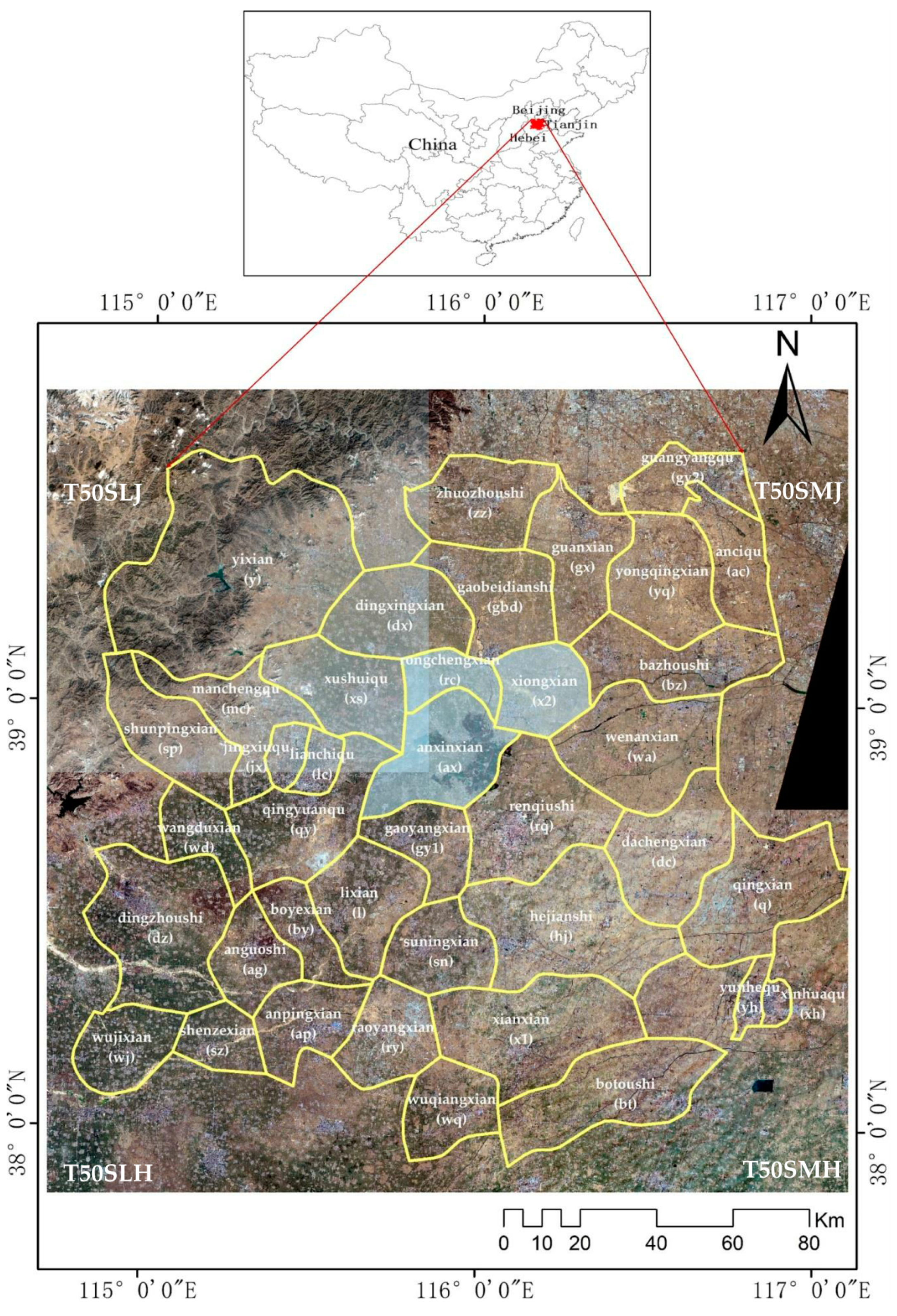
Study region and Sentinel-2 data. On the bottom, the background represents true color images of four tiles of Sentinel-2 data of which the names are shown in the corners; Yellow line refers to the boundaries of 39 counties of which names are displayed in white; letters in the brackets refer to short names of the counties; three counties with light blue refer to the core of the Xiong’an new area. Only the region covered by the Yellow lines will be used in our study.
Figure 1.
Study region and Sentinel-2 data. On the bottom, the background represents true color images of four tiles of Sentinel-2 data of which the names are shown in the corners; Yellow line refers to the boundaries of 39 counties of which names are displayed in white; letters in the brackets refer to short names of the counties; three counties with light blue refer to the core of the Xiong’an new area. Only the region covered by the Yellow lines will be used in our study.
Figure 2.
The workflow of the Fully Convolutional Network (FCN)-based method is shown on the top; the bottom illustrates the FCN model. The blue boxes indicate image features with their sizes shown in the box. Color bars represent modules with specific functions as explained at the lower-left corner.
Figure 3.
Illustration of detected increases of HRBs between 2017 and 2019; red blocks show detected increases of HRBs; green rectangles show five areas indexed in yellow for validation.
Figure 3.
Illustration of detected increases of HRBs between 2017 and 2019; red blocks show detected increases of HRBs; green rectangles show five areas indexed in yellow for validation.
Figure 4.
Overlay the increased HRBs on high spatial resolution images for visual validation; Red polygons refer to detected increases of HRBs; Yellow arrows refer to False Alarms; Green arrows refer to omitted increases of HRBs. The indexes of the areas are shown at the bottom-left corner in bold white. Nearly all omissions and commissions are HRBs with relatively small areas.
Figure 5.
Map of the area (m2) of increased HRBs at the county level; the value descends as the color turns from red to blue. To facilitate the analysis, the area of increased HRBs is graded into eight levels.
Figure 5.
Map of the area (m2) of increased HRBs at the county level; the value descends as the color turns from red to blue. To facilitate the analysis, the area of increased HRBs is graded into eight levels.
Figure 6.
The scatter plot of the block number and the area of increased HRBs at the county level; Abbreviations of the county names are used for illustration purpose; the line and its equation and also the correlation coefficient out of linear fitting are also illustrated.
Figure 6.
The scatter plot of the block number and the area of increased HRBs at the county level; Abbreviations of the county names are used for illustration purpose; the line and its equation and also the correlation coefficient out of linear fitting are also illustrated.
Figure 7.
The box and whisker plot indicates the impact of the five selected factors on the increase of HRBs, and the impact is measured by permutation importance computed by Random Forest model trained on the statistics of 39 counties. The horizontal axis refers to the normalized feature importance. The factor with larger number is more important for the increase of HRBs.
Figure 8.
The scatter plot of the volume of Gross Domestic Product (GDP) and the area of increased HRBs at the county level; the line and its equation and also the correlation coefficient out of linear fitting are illustrated.
Figure 8.
The scatter plot of the volume of Gross Domestic Product (GDP) and the area of increased HRBs at the county level; the line and its equation and also the correlation coefficient out of linear fitting are illustrated.
Table 1.
List of dates of Sentinel-2 images used in the experiment, e.g., 03–09 refers to 9 March.
Table 1.
List of dates of Sentinel-2 images used in the experiment, e.g., 03–09 refers to 9 March.
| | Tiles | T50SLJ | T50SLH | T50SMH | T50SMJ |
|---|
| Year | |
|---|
| 2017 | 03–09 | 03–09 | 03–06 | 02–24 | 03–09 |
| 2019 | 03–14 | 03–14 | 03–06 | 03–06 | 01–23 |
Table 2.
Description of five selected factors related to the increase of High-Rising Buildings (HRBs) at the county level.
Table 2.
Description of five selected factors related to the increase of High-Rising Buildings (HRBs) at the county level.
| Factor | Description |
|---|
| GDP | On the basis of GDP (billion) of the county in 2016, 6 levels are graded as follows.
Level 1: 0 < a ≤ 10, Level 2: 10 < a ≤ 20, Level 3: 20 < a ≤ 30, Level 4: 30 < a ≤ 40, Level 5: 40 < a ≤ 50, Level 6: 50 < a ≤ 60. |
| Population | On the basis of permanent residents (10,000) of the county in 2016, 5 levels are graded as follows.
Level 1: 0 < b ≤ 30, Level 2: 30 < b ≤ 60, Level 3: 60 < b ≤ 90, Level 4: 90 < b ≤ 120, Level 5: 120 < b ≤ 150. |
| Accessibility | On the basis of the total distance (km) from the political center of each county to the political center of Baoding, Beijing, and Tianjin respectively, 5 levels are graded as follows. Distance between two regions is measured by the length of optimal highway path suggested by the Baidu Map.
Level 1: c > 600, Level 2: 500 < c ≤ 600, Level 3: 400 < c ≤ 500, Level 4: 300 < c ≤ 400, Level 5: c ≤ 300. |
| Terrain | On the basis of percentage of areas with a slope equal to or higher than 15 degree in the county, 4 levels are graded as follows.
Level 1: d > 40%, Level 2: 20% < d ≤ 40, Level 3: 0 < d ≤ 20, Level 4: d = 0. |
| Policy | On the basis of governmental policy issued to regulate the construction in the center of the Xiong’an new area, 3 levels are graded as follows.
Level 1: the strictest control over construction, Level 2: medium level control over construction, Level 3: nearly no control over construction. |
Table 3.
Graded values of five selected factors for 39 counties under study; each factor is described in
Table 2.
Table 3.
Graded values of five selected factors for 39 counties under study; each factor is described in
Table 2.
| Name | GDP | Population | Accessibility | Terrain | Policy |
|---|
| anciqu | 2 | 2 | 4 | 4 | 3 |
| anguoshi | 2 | 2 | 2 | 4 | 3 |
| anpingxian | 2 | 2 | 2 | 4 | 3 |
| anxinxian | 1 | 2 | 4 | 4 | 1 |
| bazhoushi | 4 | 3 | 5 | 4 | 2 |
| botoushi | 3 | 3 | 2 | 4 | 3 |
| boyexian | 1 | 1 | 2 | 4 | 3 |
| dachengxian | 2 | 2 | 3 | 4 | 3 |
| dingxingxian | 2 | 3 | 4 | 4 | 2 |
| dingzhoushi | 4 | 5 | 2 | 4 | 3 |
| gaobeidianshi | 2 | 2 | 4 | 4 | 2 |
| gaoyangxian | 1 | 2 | 4 | 4 | 2 |
| guanxian | 3 | 2 | 4 | 4 | 2 |
| guangyangqu | 3 | 2 | 4 | 4 | 3 |
| hejianshi | 3 | 3 | 3 | 4 | 3 |
| jingxiuqu | 2 | 2 | 4 | 4 | 2 |
| lixian | 1 | 2 | 3 | 4 | 2 |
| lianchiqu | 5 | 3 | 4 | 4 | 2 |
| manchengqu | 2 | 2 | 3 | 2 | 3 |
| qingxian | 2 | 2 | 3 | 4 | 3 |
| qingyuanqu | 2 | 3 | 4 | 4 | 2 |
| raoyangxian | 1 | 1 | 2 | 4 | 3 |
| renqiushi | 6 | 3 | 4 | 4 | 2 |
| rongchengxian | 1 | 1 | 4 | 4 | 1 |
| shenzexian | 2 | 1 | 1 | 4 | 3 |
| shunpingxian | 1 | 2 | 3 | 1 | 3 |
| suningxian | 2 | 2 | 3 | 4 | 3 |
| wangduxian | 1 | 1 | 3 | 4 | 3 |
| wenanxian | 2 | 2 | 4 | 4 | 2 |
| wujixian | 2 | 2 | 1 | 4 | 3 |
| wuqiangxian | 1 | 1 | 1 | 4 | 3 |
| xianxian | 3 | 3 | 2 | 4 | 3 |
| xinhuaqu | 2 | 1 | 3 | 4 | 3 |
| xiongxian | 2 | 2 | 4 | 4 | 1 |
| xushuiqu | 2 | 3 | 4 | 3 | 2 |
| yixian | 2 | 2 | 3 | 1 | 3 |
| yongqingxian | 2 | 2 | 5 | 4 | 3 |
| yunhequ | 3 | 2 | 3 | 4 | 3 |
| zhuozhoushi | 3 | 3 | 4 | 4 | 3 |
Table 4.
Results of all five validation areas based on the number of increased HRBs block. Each block is a polygon referring to a spatial connected cluster of the increased HRBs. GT, OA, FA—Ground Truth, Overall Accuracy, and False Alarm, respectively.
Table 4.
Results of all five validation areas based on the number of increased HRBs block. Each block is a polygon referring to a spatial connected cluster of the increased HRBs. GT, OA, FA—Ground Truth, Overall Accuracy, and False Alarm, respectively.
| No. | GT Number | OA Percentage (Number) | FA Percentage (Number) | Average FA Percentage | Average OA Percentage |
|---|
| A1 | 21 | 90.48%(19) | 4.76%(1) | 8.25% | 95.87% |
| A2 | 18 | 88.89%(16) | 5.55%(1) |
| A3 | 7 | 100%(7) | 14.28%(1) |
| A4 | 6 | 100%(6) | 16.67%(1) |
| A5 | 21 | 100%(21) | 0%(0) |
© 2020 by the authors. Licensee MDPI, Basel, Switzerland. This article is an open access article distributed under the terms and conditions of the Creative Commons Attribution (CC BY) license (http://creativecommons.org/licenses/by/4.0/).


