Probabilistic Fire Risk Framework for Optimizing Construction Site Layout

Abstract

Purpose: This paper aims to develop an efficient model able to reduce catastrophic consequences and the significant number of victims resulting from fires at construction sites. The paper proposes probabilistic modeling aimed to minimize the probability of failure of a construction site. Methodology: The developed model in this paper consists of modeling fire hazards, the vulnerability of the potential targets, and the risk within construction sites. The optimization algorithm called “differential evolution” is used in order to determine the optimal site layout, which is characterized by having the smallest overall probability of failure. A numerical simulation is performed to delineate an appropriate probability density function of the failure of the site. In addition, a geographic information system (GIS) is used to display the spatial variability of fire risk on a construction site. Findings: The paper provides an efficient model to enhance site layout planning and assign locations for supporting temporary facilities at appropriate positions within a construction site. The model is examined through applying it on a simple case study containing numerous facilities. All these facilities are considered vulnerable targets and some of them are potential fire hazards, with different intensity values. Value: Most of the previous research focuses on travel cost distance in developing site layout planning models. This paper fulfills the development of a valuable model able to generate an optimized construction site layout by minimizing the probability of failure of the whole site. It will assist the decision makers and the risk managers in identifying the riskiest zones on a construction site.

1. Introduction

A construction site contains several supporting temporary facilities such as a concrete plant, tower crane, materials storage area, electrical generator, and fuel storage. These facilities are necessary to execute construction activities. Construction sites, like any other industry sites, are susceptible to the occurrence of fires due to the use of hazardous materials or the use of advanced technology in performing construction activities. A fire may occur in one or several supporting facilities. They may damage the construction site completely or partially. Whatever damage level occurs, in the construction site, the work in the site will be suspended. Construction managers always do their best to restrain the expected serious consequences of a fire to a minimum level. According to references [1,2], fire is one of the accidental events that may hinder completing a construction project within a preplanned time and budget. Reference [3] indicated that the frequent occurrence of fires at construction sites can be attributed to the fast development of the construction methods. The National Fire Protection Association (NFPA) pointed out that, during the period between 2013 and 2017, the average number of fires that occurred yearly in buildings under construction was 3840. These fires approximately yielded $304 million of losses in assets.

It is obvious from these data: there is an urgent need to minimize the losses and consequences of this kind of hazard. One creative way to achieve this purpose is to place temporary facilities at an appropriate available space on a construction site i.e., optimizing site layout planning. References [4,5,6] declared that appropriate site layout planning is highly significant to the success of large-scale construction projects and leads to safe work environments. In addition, reference [7] stated that the success of a construction project is closely related to the proper construction site layout planning.

Reference [8] stated that productivity can be enhanced by developing a well-organized site layout. References [9,10] found that the principle “first come first served” is the most common tactic utilized by construction planners for arranging the construction site layout, and they entirely focused on diminishing the travel cost distance among facilities. In addition, the majority of the current models for arranging temporary facilities on a construction site disregard the expected risk of fires, which may result in generating an unsafe site environment, which in turn leads to damage to one or more supporting facilities and even the whole construction site.

Very few previous works devoted to generating site layout planning models considered potential hazards. Reference [9] developed a model that aims to maximize a safe work environment by focusing on facilities containing hazardous materials and secluding these facilities a sufficient distance from other facilities. Reference [11] developed a generalized deterministic model to reduce the risk of potential hazards. Reference [12] suggested a multi-objective mathematical optimization model with fuzzy parameters and simulation. The proposed model has been implemented on a large-scale project and it appears it is effective in enhancing safety and operation efficiency at the construction site. Clearly, safety concerns related to fire risk were not deeply addressed in site layout planning in previous studies. Consequently, there is a great necessity to develop a creative model aimed to arrange the construction site in order to minimize the losses in both lives and assets during emergency cases.

Firstly, this research drew inspiration from reference [13] who stated that a hazardous condition is a consequence of interacting and counteracting characteristics of labor. However, in the current study, the hazardous situation is referred to as the interaction among facilities on a construction site.

Moreover, the current study aimed to find the optimal site layout by minimizing the catastrophic consequences of a potential fire hazard. In addition, a geographic information system (GIS) has been utilized to display the spatial variability of risk in a map format. This map plays a primary role in adopting proper decisions by managers.

It is worth noting here that the implementation of the proposed model is limited to regular construction sites and facilities. Moreover, the possibility of facilities’ positions changing over time is not allowed.

2. Literature Review

References [14,15,16] confirmed that site layout planning is complex work and it is still a scientific challenge. In general, a lot of effort has been exerted by researchers to enhance construction site layout planning. Most of these efforts have been directed toward either minimizing travel cost distance among facilities [14,17,18,19,20,21,22,23,24] or maximizing safe work environments by considering the safe operation of some supporting facilities, cranes for instance, and give a higher priority of control on the facilities containing hazardous material [8,9,13,15,25,26,27]. They also applied numerous algorithms to accommodate facilities on a construction site. According to references [28,29], the adopted algorithms utilized to enhance and solve the problem of site layout planning can be categorized into four classes: improvement, construction, graph-theoretic, and hybrid algorithms. Reference [30] developed an optimization model combining a max–min ant system with a genetic algorithm. Reference [31] stated that the most common algorithms used for site layout optimization are ant colony, simulated annealing, and genetic algorithms (GAs). Reference [32] established a new numerical mathematical programming model to improve the optimality of site layout planning. They made a comparison between their suggested model and the existing heuristics model. The results indicated that their model achieves about 3% to 19% improvement on optimality over the existing heuristics models. Reference [33] reviewed heuristic and non-heuristic methods for construction site layout planning. They established a framework for allocating temporary facilities in a hilly region.

References [20,21] used the search by elimination principle to identify the best position for each temporary facility. Reference [22] developed an EvoSite model to generate an optimal layout. Reference [10] proposed a dynamic programming optimization model aiming to decrease the overall site layout costs. Reference [17] generated an innovative optimization model based on the principles of energy governing the physical system. Reference [19] used building information modeling to create a 3D site layout.

Reference [25] took into account the travel cost distance, site safety, and productivity as criteria to generate an optimal layout. Reference [15] considered the safety aspects and the actual routes between supporting facilities as the main criteria for a site layout. Reference [5] developed a quantitative safety risk assessment model to evaluate site layout plans in a holistic manner. It helps site managers make proper decisions when they face different site layout scenarios. Reference [9] generated a model able to minimize travel cost distance and maximize construction site safety. They considered the crane and hazardous materials as being the main causes of hazardous situations on construction sites. Thus, they proposed keeping away these two sources of hazard at a sufficient distance from other facilities. References [4,12,34] proposed an efficient bi-level mathematical site layout model for a dam construction project. The model aims to enhance construction operations and save costs. Reference [6] developed a multi-objective site layout optimization model to improve safety in construction sites. They consider potential risks resulting from facility interaction relationships, geographic hazardous sources relationships, and travel cost distances as the objective function in their model. Reference [35] presented a multi-objective optimization model for optimizing site layout planning to minimize the effect of explosive attacks at remote construction sites. The model aims to minimize site construction costs and facility damage levels. Reference [7] highlighted the latest advanced technologies used on site layout planning for prefabricated construction. Reference [36] designed an optimization site layout model to minimize noise pollution resulting from construction activities on construction sites.

Furthermore, other researchers devoted their attention to developing frameworks aimed to quantify the vulnerability, the incurred losses, and the probability of failure of the systems due to the occurrence of natural hazards, such as floods, tsunamis, earthquakes, and landslides [37,38,39,40,41,42,43,44,45,46,47,48,49].

Reference [38] stated that the risk is quantitatively measured in physical science, while it is qualitatively measured in social sciences. Reference [50] indicated that fires are the primary incidents for the occurrence of domino effects. Reference [41] investigated the domino effects that may take place in industrial plants. They proposed simplified mechanical models to describe global failure of tanks in a plant. Reference [42] studied the failure risk of masonry construction due to flood hazards. References [43,44] studied the risk of a tsunami on coastal industrial tanks and evaluated resilience after its occurrence. Reference [39] developed a probabilistic approach to quantify the probability of failure due to explosions in industrial plants. Reference [46] presented a methodology to quantify the individual and societal risk of domino effects triggered by fire and explosions in an industrial site. Reference [40] assessed the risk due to a domino effect in order to identify the potential escalation of hazard events in industrial areas. Reference [45] proposed a procedure to minimize the probability of a domino effect in industrial areas. It is based on the assumption that the layout should be adequate to diminish the escalation probability of a hazard. Reference [49] developed a GIS-based model capable of visualizing the variability of potential damages and casualties of coastal areas prone to tsunamis. Reference [48] studied the hazard, vulnerability, and risk analysis for buildings prone to tsunamis in Alexandria. Reference [37] discussed the reasons behind poor modeling of physical vulnerability for most kinds of natural hazards, which impact the accuracy of risk estimations. Reference [47] developed a set of fragility curves in order to quantify potential losses due to tsunami. These curves show the relationship between tsunami wave height and mean damage intensities for buildings prone to tsunami by the Indian Ocean. Reference [51] generated a stochastic approach to estimate the expected damages of buildings due to seismic events. Reference [52] derived the vulnerability curve of concrete buildings due to a debris-flow hazard. They found that vulnerability is highly dependent on the type of construction material utilized in buildings. Reference [53] investigated the vulnerability of typical buildings to earthquakes and display their variation of damage rate in a map form. Reference [54] used two methods to evaluate the seismic risk of buildings: a vulnerability index and a capacity spectrum. Reference [55] assessed the seismic risk in a probabilistic manner. Reference [56] developed a scientific platform model called CAPRA to minimize the potential damages of hazard. Reference [57] suggested a conceptual extension to the existing risk assessment models in order to standardize the consequences of hazard evaluations.

It is obvious that very few studies have been dedicated to developing an optimal site layout taking into account the consequences of natural or technological hazards of the failure of the site. In addition, these few existing studies are deterministic in nature. They are not reflecting the reality, because they ignored a lot of uncertainties associated with hazards and the vulnerability of elements at risk (temporary supporting facilities in our case). Thus, this research aimed to develop a probabilistic optimization model able to minimize the probability of failure of the whole site. The risk of failure, in the current research, is assumed to be a combination of the individual failure of each facility on the construction site. Moreover, the proposed model aimed to display the propagation of uncertainty in the probability of failure of the whole site. Furthermore, the geographic information system (GIS) was used in order to perform a spatial analysis process and develop a spatial fire risk map in the construction site. The proposed model will assist construction managers in ordering facilities based on their probability of failure in determining the facilities that required more attention. This, in turn, will lead to enhancing safety and constructability during the construction phase.

3. Methodology

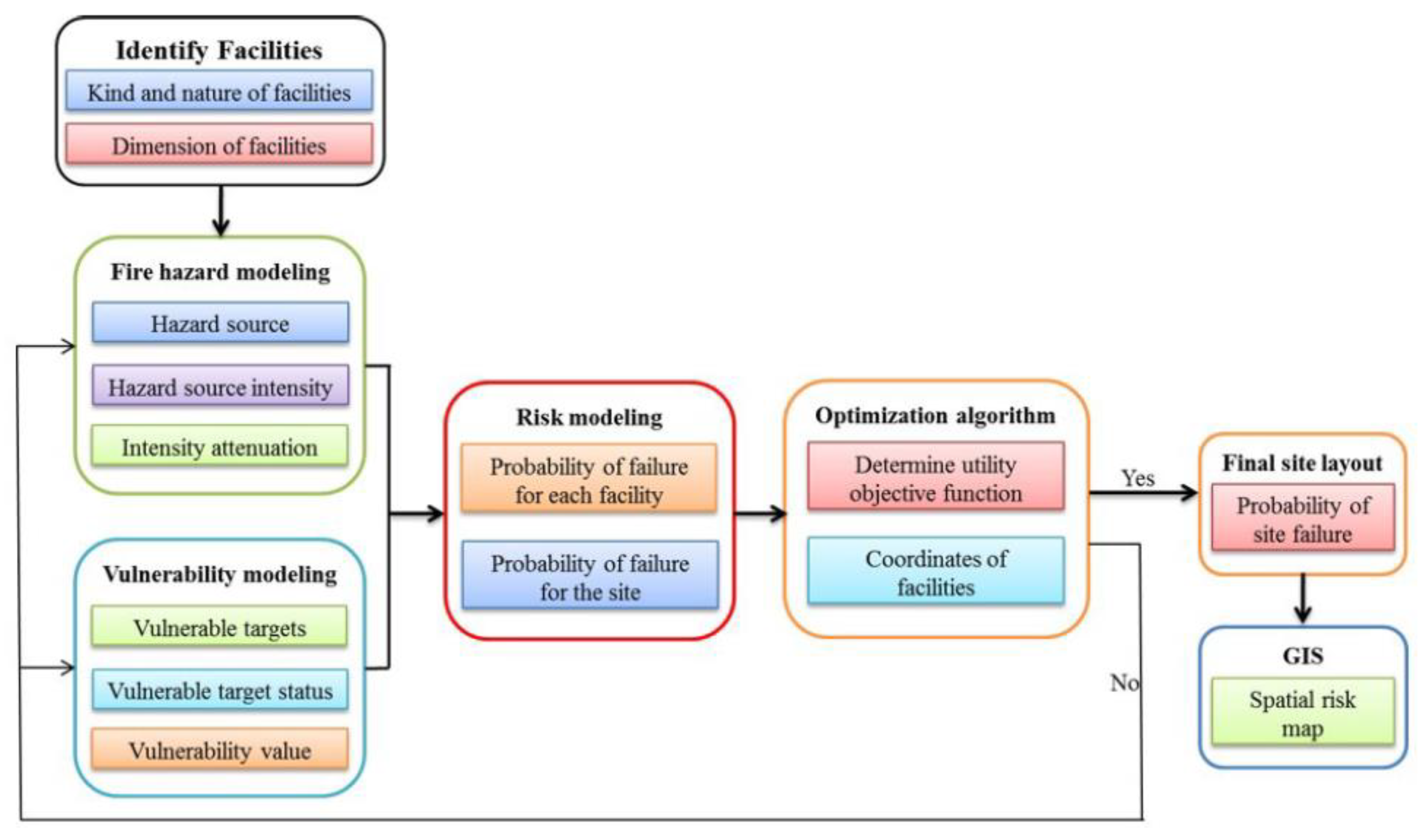
Figure 1 displays the methodology adopted to generate an optimal site layout. It consisted of several steps: (1) identifying the characteristics of the required facilities to be set up on a construction site, (2) hazard modeling, (3) vulnerability modeling, (4) risk modeling, (5) using optimization technique, (6) generate spatial risk map utilizing GIS.

Particularly, fire hazard modeling consisted of identifying (a) the hazard sources, i.e., the facilities that trigger the occurrence of the fire; (b) the fire hazard intensity of the hazardous sources through probabilistic density function; (c) the attenuation model that displays the propagation of the fire hazard and its intensity on the impacted targets. On the other hand, the vulnerability modeling involved (a) identifying the potential targets that may be impacted by the hazard; (b) identifying the vulnerability status of each target; (c) estimating the conditional vulnerability value utilizing vulnerability damage functions, which express the vulnerability vs. the fire hazard intensity.

Furthermore, risk modeling represents the probability of failure or damage to the whole construction site. This probability of loss was obtained by concatenating hazard and vulnerability of elements at risk (i.e., facilities on a construction site). The probability of failure of the whole site is a combined effect of the individual failures of all facilities on the site. The purpose of the utilization of an optimization algorithm was to minimize the probability of failure of the whole site through finding the best coordinates (x, y) of all facilities at the available spaces within a construction site and without overlapping them. Once the optimal site layout was generated, the GIS spatial analysis function was utilized to develop a spatial risk map that discerns the risk’s variation in a construction site.

3.1. Facility Identification

Usually, construction manager and planner identify, in advance, the required supporting facilities to execute production activities. Identification of the kind and nature, as well as the dimensions, of these facilities are essential in order to locate them in the best position in a construction site. In this research, whatever the case, the supporting facilities (offices, material storage, concrete plant, fuel storage, electrical generator, for instance) were represented as a rectangular object with length (ℓ_i) and width (w_i) in a 2D layout.

3.2. Hazard Modeling

Fire is one kind of threat that could cause damage to the construction project. Similar to any other kind of hazard, modeling fire hazard involves several uncertainties; one of these uncertainties starts through identifying the potential facilities responsible for the initial spark of fire accident. These facilities are most hazardous compared to others. Usually, the electrical generator, the fuel storage, and the chemical materials are the most prone to fire occurrence. As it is not easy to anticipate which facilities are responsible for the occurrence of the initial accident, hence, it was assumed that the initial fire accident event would occur in all of them simultaneously if they existed in a construction project. This assumption considered the probable worst-case scenario. Another uncertainty associated with fire hazard modeling consisted of estimating the fire intensity at the initial hazard sources. Fire intensity can be defined as the amount of energy emanating from each meter of head fire edge; it can be expressed in kilowatt per meter (kW/m). It depends on the amount of flaming material and the burning speed. Specifically, the fire hazard intensity was classified into four categories, ranging from low scale to very high scale grade, as specified in

Table 1. Categories of fire hazard intensity [58].

Fire Hazard Level	Fire Intensity (kW/m)	Fire Flame Height (m)
Low hazard	Less than 400	0–1.5
Medium hazard	400–less than 1000	1.5–7
High hazard	1000–less than 2000	7–14
Very high hazard	Greater than 2000	>14

[58].

The expected fire hazard level for each hazardous facility was identified on the basis of historical data or expert judgment. Thus, in case the historical data was not available, subject matter experts had to identify the fire hazard level for each facility depending on the categories shown in Table 1. It is obvious from Table 1 that each fire hazard level fell within a range of fire intensity values (minimum and maximum value for each hazard level). Therefore, it was assumed that, for each fire hazard level, the fire intensity was a random variable which followed a uniform probability density function (i.e., if the fire hazard level for one facility was specified to be medium, then the fire intensity value for that facility had a uniform random variable range between 400 and 1000 kW/m).

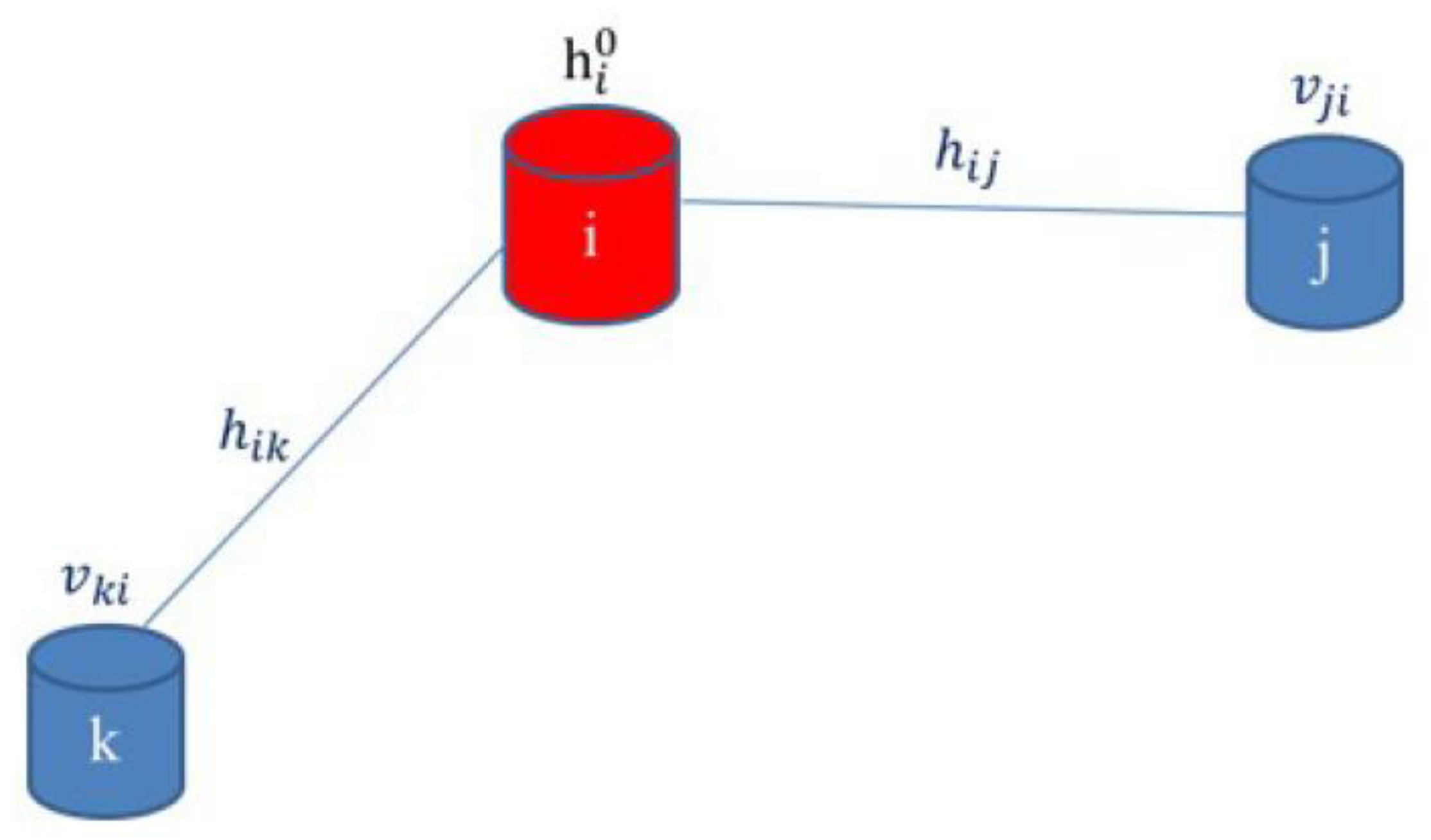
In fact, due to the wind motion and other fire phenomena characteristics, fire propagates to impact other erected facilities, but with intensity values less than that at the initial hazard sources, due to attenuation of hazard with distance. Figure 2 shows that if the fire hazard initiates at object (i) with intensity ($h_i^0$), later the fire propagates to impact on objects (j) and (k) with intensities ($h_{ij}$) and ($h_{ik}$) respectively. 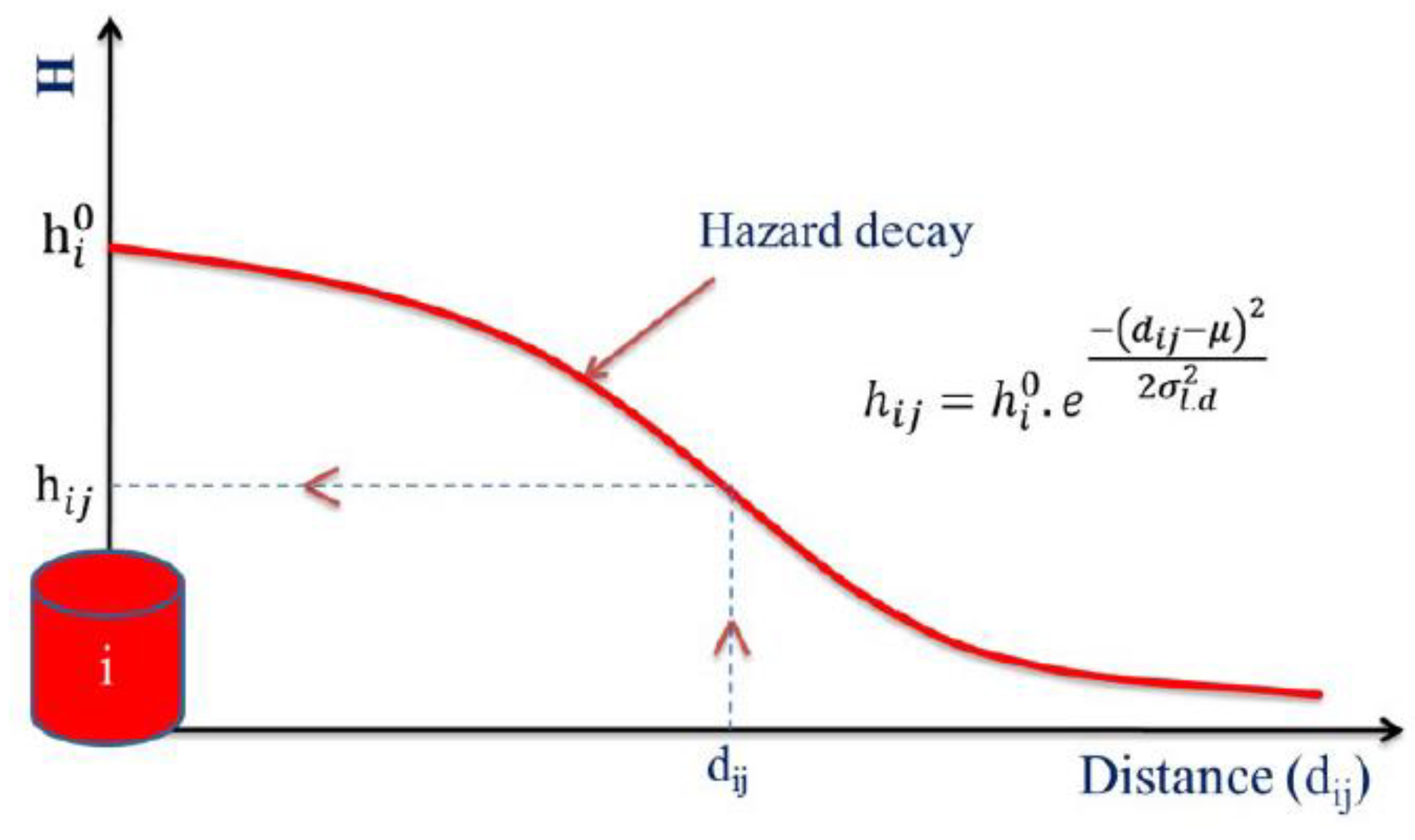Surely, these two hazard intensities are smaller than the initial fire intensity value at object (i) due to attenuation law. Due to lack of past accident feedback (historical information), it was assumed that the attenuation of fire hazard intensity follows a normal distribution function, as shown in Figure 3 which displays the relation between fire hazard intensity and distance (i.e., the initial hazard intensity arising from facility i decreases with distance (d_ij), its intensity value on a potential target j equal to ($h_{ij}$), which is surely less than $h_i^0$).

To construct hazard matrix H, suppose there is (n) number of facilities needed to be set up on a construction site. Consequently, the hazard matrix of size (n × n) should be created. Equations (1)–(5) show the hazard matrix that displays the impact of each facility on itself as well as on other erected facilities [26,27]. The diagonal values of the matrix represent the fire hazard intensity of each facility on itself. They were selected randomly from a uniform density function based on the specified hazard level for that facility.

In fact, for each row in the matrix, the diagonal value is the highest one compared to others, since the hazard is highest at its origin and its impact on the surrounding objects decreases with distance. This can be seen in Equations (6)–(8) [26,27].

$$H=\left[\begin{array}{ccc}{h}_{11}& \dots & h_{1n}\\ ⋮& h_{ij}& ⋮\\ h_{n1}& \dots & h_{nn}\end{array}\right]$$

(1)

Due to probabilistic description of the model, the hazard matrix is normalized using Equations (2)–(5).

$$H^{*}=\left[\begin{array}{ccc}{h}_{11}^{*}& \dots & h_{1n}^{*}\\ ⋮& h_{ij}^{*}& ⋮\\ h_{n1}^{*}& \dots & h_{nn}^{*}\end{array}\right]$$

(2)

$$H=\max \left[h_i^0\right]. H^{*}=\max \left[h_i^0\right]. \left[\begin{array}{ccc}{h}_{11}^{*}& \cdots & h_{1\mathrm{n}}^{*}\\ ⋮& h_{ij}^{*}& ⋮\\ h_{\mathrm{n}1}^{*}& \cdots & h_{\mathrm{nn}}^{*}\end{array}\right]$$

(3)

$$h_{ij}^{*}=\frac{h_{ij}}{\max \left[h_i^0\right]}$$

(4)

$$h_i^0=h_{ii}$$

(5)

$$h_{ij}=h_i^0. e^{\frac{-{\left(d_{ij}-\mu \right)}^2}{2{\sigma }_{l.d}^2}}$$

(6)

$$h_{ij}^{*}=P\left(H_i^0=h_i^0\right). P\left(H_{ij=}{h_{ij}|}_{d_{ij}}\right)$$

(7)

$$P\left(H_i^0=h_i^0\right)=\frac{h_i^0}{\max \left[h_i^0\right]}$$

(8)

$$d_{ij}=\sqrt{{\left(x_i-x_j\right)}^2+{\left(y_i-y_j\right)}^2}$$

(9)

where:

H: is a hazard matrix that displays the impact of each facility on itself as well as on other surrounding facilities

$H^{*}$: is a normalized matrix of the fire hazard

$h_{ij}$: is the intensity of fire hazard at facility (j) due the fire hazard arising at facility (i)

$h_{ij}^{*}$: is a normalized fire hazard intensity at facility (j) due to the fire hazard arising at facility (i), $\forall h_{ij}^{*}\in \left[0,1\right]$

$\max \left[h_i^0\right]$: is the highest value of fire hazard intensity arising at facility(i) at distance (d_ij = 0) among all hazardous facilities, its maximum value appears in the diagonal of the hazard matrix

$h_i^0=h_{ii}$ : is the value of fire hazard intensity arising at facility (i) at distance (d_ij = 0), i.e., the impact of facility on itself

$d_{ij}$ : is the shortest distance between facilities (i) and (j), i.e., Euclidean distance

$x_i, y_i, x_j, y_j$: are the coordinates of facilities “i” and “j”

n: is the number of facilities needed to be set up on a construction site

$P\left(H_i^0=h_i^0\right)$ : is the probability of fire hazard intensity arising at facility (i)

$P\left(H_{ij=}{h_{ij}|}_{d_{ij}}\right)$: is the probability of fire hazard intensity at the facility(j) due to the fire hazard arising at the facility (i)

$\mu ,{\sigma }_{l.d}$: The mean and standard deviation of distance respectively. These are the parameters of hazard attenuation model, which is assumed to be a normal distribution. They can be obtained from either experimental or historical data.

3.3. Physical Vulnerability Modeling

Vulnerability can be defined as the susceptibility of exposed element at risk to suffer a loss as a consequence of hazard occurrence. Modeling vulnerability involves a lot of uncertainties, such as identifying the potential targets that may be impacted by the hazard, the status of these targets, and their expected level of damage. The physical vulnerability of each target object depends on its capacity to withstand and resist different hazard values arising from surrounding objects. Usually, all of the erected facilities in construction site are considered to be potential targets that will be impacted by fire hazard occurrence. These potential targets are vulnerable to damage with different damage levels ranging from 0 (no destruction) to 1 (completely destruction). This damage level depends on the intensity of the hazard, the ability of facilities to resist the hazard, and the distance of the facilities from the hazard sources. Thus, the damage level or conditional vulnerability is defined as the probability that the limit state value (the difference between the resistance R of the object and the hazard intensity (h) on the object) is less than or equal to zero, given the hazard intensity is (h₀), i.e., $P\left({\left(R-h\right)|}_{h_0}\right)$.

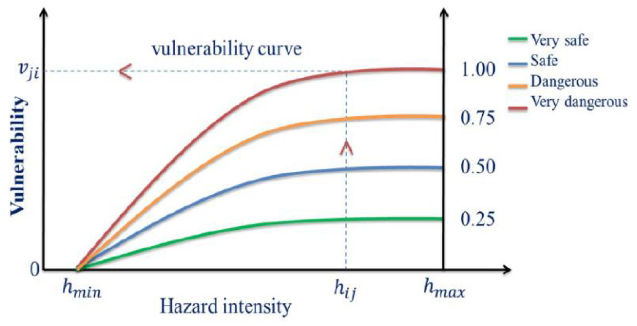
Generally, in order to estimate the vulnerability of a specific type of element at risk subjected to a specific kind of hazard, vulnerability curves can be used. These curves are developed based on historical or experimental data. They can be considered as mathematical functions showing the relation between the damage level and the hazard intensity. In fact, it is easy to find this kind of curve for masonry or reinforced structures prone to earthquake and/or flood hazard. In contrast, for fire, these curves are not available for both permanent and temporary facilities. Therefore, the vulnerability assessment in this research was done using the semi-quantitative method proposed by authors of [42]. They presented vulnerability as a function of hazard intensity. They stated that typical damage curves are displayed in an elliptic shape as shown in Figure 4. In addition, Figure 4 displays the maximum damage level value for each damage state.

For vulnerability assessment in the current model, experts were requested to classify each temporary facility into one of four classes (very safe, safe, dangerous, and very dangerous). For each class, a maximum conditional vulnerability was assigned. Afterward, an ellipsoidal function was utilized to estimate the conditional vulnerability for each facility as displayed in Equation (10). This Equation shows how conditional vulnerability evolved concerning hazard intensity. Based on this Equation, the vulnerability interaction matrix V with size (n × n) was established as shown in Equation (11).

$${\left(\frac{P\left({v_{ji}|}_{h=hij}\right)}{P\left(v_{max}\right)}\right)}^2+{\left(\frac{h_{\max }-h_{ij}}{h_{\max }}\right)}^2=1$$

(10)

$$V=\left[\begin{array}{ccc}P\left({v_{11}|}_{h=h_{11}}\right)& \dots & P\left({v_{1n}|}_{h=h_{n1}}\right)\\ ⋮& P\left({v_{ji}|}_{h=h_{ij}}\right)& ⋮\\ P\left({v_{n1}|}_{h=h_{1n}}\right)& \dots & P\left({v_{nn}|}_{h=h_{nn}}\right)\end{array}\right]$$

(11)

where:

V: is the vulnerability matrix that displays the ability of potential targets to resist different hazard values arising from surrounding objects

${\mathrm{v}}_{ji}$ : is the ability of vulnerable target (j) to withstand and resist the hazard arising at facility (i)

$P\left({v_{ji}|}_{h=hij}\right)$: is corresponding conditional probability of damage for facility (j) as a result of hazard generated by facility (i), given hazard intensity at j equal to $h_{ij}$, it ranges between 0 (no destruction) to 1 (completely destruction)

$P\left(v_{\max }\right)$: is the maximum expected damage level of the facility based on its classification

$h_{\max }$: is the maximum hazard intensity within the validity domain values of hazard

3.4. Risk of Failure

Risk is the likelihood of damage or loss in elements at risk as a result of the occurrence of a hazard. It was computed as a convolution product between hazard and vulnerability as presented in Equation (12). In the current study, it was assumed that the failure of each facility is independent of all other facilities and the failure of the whole site is a combined event of individual failure of all facilities. The mathematical workflow derivation of failure of each facility as well as of the whole site is shown in Equations (13)–(20):

$$Risk=Hazard ⨂ Vulnerability$$

(12)

Suppose the failure of the whole site is ($E_{site})$, the failure of each facility is ($E_i)$. Since the failure of the whole site is a combined event of individual failure of all facilities, then:

$$E_{site}={\displaystyle \bigcup }_{i=1}^n{E}_i$$

(13)

If the probability of failure of the whole site is given by $P\left(E\right)$, then according to probability and Demorgan laws, the safety of the site is the complement of the failure, hence:

$${\overline{E}}_{all site}={\displaystyle \bigcap }_{i=1}^n{\overline{E}}_i$$

(14)

$$P\left(E\right)=1-{\displaystyle \prod }_{i=1}^n( 1-P\left(E_i\right))$$

(15)

To estimate the probability of failure of each facility$P\left(E_i\right)$, it was assumed that the failure of each facility (i) was a combined effect of the individual impact of all other facilities on that facility (i), therefore:

$$E_i={\displaystyle \bigcup }_{j=1}^n{E}_{ij}$$

(16)

According to probability and Demorgan laws, the safety of the facility is the complement of the facility failure, therefore:

$${\overline{E}}_i={\displaystyle \bigcap }_{j=1}^n{\overline{E}}_{ij}$$

(17)

$$P\left(E_i\right)=1-{\displaystyle \prod }_{j=1}^n( 1-P\left(E_{ij}\right))$$

(18)

$$P\left(E_{ij}\right)=P\left(h_j\right). P\left({v_{ij}|}_{h_{ji}}\right)$$

(19)

By the substitution of Equations (18) and (19) in Equation (15), the probability of failure of the whole site becomes:

$$P\left(E\right)=1-{\displaystyle \prod }_{i=1}^n\left({\displaystyle \prod }_{j=1}^n\left(1-P\left(h_j\right). P\left({v_{ij}|}_{h_{ji}}\right)\right)\right)$$

(20)

where:

$P\left(E\right)$: is the probability of failure of the whole construction site

$P\left(E_i\right)$: is the probability of failure of facility (i)

$P(E_{ij})$: is the probability of failure of facility (i) due to the impact of facility (j) on it

$P\left(h_j\right)$: is the probability of hazard arising at facility (j)

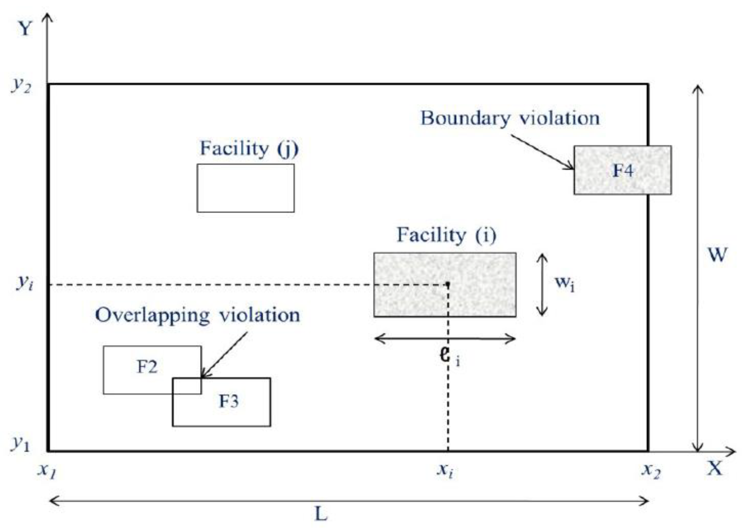
3.5. Site Representation, Constraints, and Identification of Objective Function

In the current model, the rectangular shape with length (L) and width (W) is used to represent the construction site. In addition, the rectangle corners’ coordinates are also identified. As previously specified, the construction supporting facilities must be placed within a construction site without overlapping. To achieve this, the centroid coordinates (x_i, y_i) of each facility should be determined. Figure 5 shows the rectangular construction site, the rectangular construction facilities, the centroid coordinates (x_i, y_i) for the facility (i), and the boundary and overlapping constraints considered to accommodate facilities.

The proposed model aimed to develop an appropriate site layout (i.e., determining the best coordinates of each facility) able to minimize the probability of failure of the whole site. As shown in Equation (20), the probability of failure of the whole site can be minimized by maximizing the negative part of the equation that represents the safety of the whole site. Once the optimization process achieves the objective function, the final site layout can be developed. The objective function is shown in Equation (21), whereas, Equations (22)–(25) display the boundary constraint, while the mathematical formulas of overlapping constraint are presented in Equations (26) and (27) [59].

$$maximize\left({\displaystyle \prod }_{i=1}^n\left({\displaystyle \prod }_{j=1}^n\left(1-P\left(h_j\right). P\left({v_{ij}|}_{h_{ji}}\right)\right)\right)\right)$$

(21)

$$x_1+\frac{{\ell }_i}{2}-x_i\le 0.0$$

(22)

$$x_i+\frac{{\ell }_i}{2}-x_2\le 0.0$$

(23)

$$y_1+\frac{w_i}{2}-y_i\le 0.0$$

(24)

$$y_i+\frac{w_i}{2}-y_2\le 0.0$$

(25)

$$-\left|x_i-x_j\right|+\frac{{\ell }_i}{2}+\frac{{\ell }_j}{2}\le 0.0$$

(26)

$$-\left|y_i-y_j\right|+\frac{w_i}{2}+\frac{w_j}{2}\le 0.0$$

(27)

where:

${\ell }_{i,}{\ell }_{j,}{w}_i,w_j$: are the dimensions of the rectangular facilities

3.6. Optimization Technique

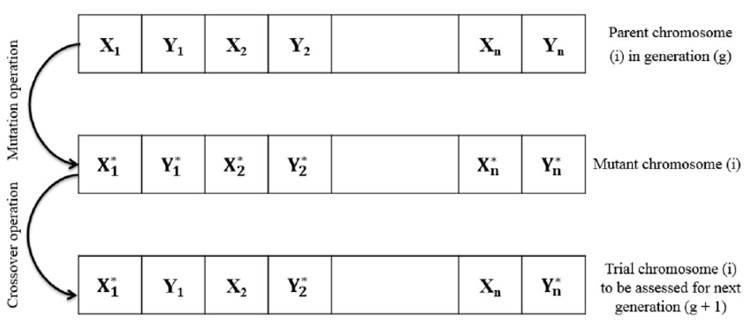
In the current framework, the optimization process was conducted in order to find the best coordinates of each facility (x, y) utilizing one of the evolutionary optimization techniques called “differential evolution”. This algorithm was implemented in a python language platform under a common library known as “science python” (SciPy). The working mechanism of the differential evolution algorithm can be derived from Figure 6. It can be noticed that the process started with the formation of several random chromosomes for each generation called “population”. Each chromosome in the population consists of genes. The number of genes in the chromosome equals to the total number of decision variables of the problem under study. In our case, the decision variables were the coordinates of the facilities that must be placed on a construction site. Hence, if the number of facilities is (n), then each chromosome consists of (2n) decision variables. Every chromosome in the population was evaluated through fitness function to check it was appropriate for the solution. In addition, the chromosomes in the population were subjected to two genetic operations called “mutation and crossover” to create new chromosomes called “off-springs” [60,61,62]. The off-springs underwent the fitness assessment, too. If the results seem better than the parents, they occupied their positions in the population to form a new generation. The process continued until the survival of the best achieved and the optimal results were obtained.

3.7. GIS Spatial Risk Map

For the sake of simplicity, it was assumed that the spaces on the site had the same ability to withstand and resist the hazard (i.e., same vulnerability conditions). In addition, they were impacted by the surrounding facilities. GIS is an essential tool to enhance decision making. It was used, in the current model, to convert construction site and facilities into raster. The raster values for facilities represented the probability of failure for that facility $\left(z_i\right)$. Moreover, it was also used to run inverse distance weighting (IDW) process, which is one of the interpolation techniques that is already included in GIS. The purpose of performing the interpolation process was to estimate the probability of failure of each unknown cell (${\mathcal{Z}}_k$) within the site and develop the spatial risk map. Equations (28) and (29) explain the working mechanism of the IDW technique and the way to estimate (${\mathcal{Z}}_k$).

$$w_i=\frac{1}{d_{ik}^p}$$

(28)

$${\mathcal{Z}}_k=\frac{{{\displaystyle \sum }}_{i=1}^m{z}_i{w}_i}{{{\displaystyle \sum }}_{i=1}^m{w}_i}$$

(29)

where:

${\mathcal{Z}}_k$: is the probability of failure of cell (k) within the site

$z_i$ : is the probability of failure of the cell (i) that representing the facility, it is used as sample interpolated point

$w_i$ : is the importance of sample point (i)

$d_{ik}$ : is the distance between the unknown node (k) and the sample interpolated point (i)

p: is a power value parameter (p ≥ 1)

m: is the total number of sample interpolated points utilized to estimate the probability of failure of the unknown node (k)

4. Model Implementation

The proposed model was implemented on a case study in order to examine its adequacy and ability for developing a site layout which minimizes the probability of failure of the whole site. The case study was composed of nine facilities with different dimensions and characteristics. It was required to accommodate these facilities in a construction site with dimensions (55 × 55 m). The nature, dimensions, and characteristics of these facilities are displayed in

Table 2. Facilities’ description and characteristics.

Facility	Nature of Facility	$\mathbf{Length}“\mathbf{\ell }”\left(\mathbf{m}\right)$	Width “w” (m)	Movable or Fixed	Hazard Source	Hazard Level	Vulnerability Class
F1	Electric generator	2	1	Movable	Yes	High	Safe
F2	Labor services	7	3	Movable	No	---	Very dangerous
F3	Concrete plant	10	6	Movable	No	---	Dangerous
F4	Job office 1	12	5	Movable	No	---	Very dangerous
F5	Job office 2	5	12	Movable	No	---	Very dangerous
F6	Steel storage	8	20	Movable	No	---	Safe
F7	Fuel storage	2	1	Movable	Yes	High	Safe
F8	Tower crane	8	8	Fixed (32, 30) *	No	---	Safe
F9	Construction building	26	50	Fixed (14, 28) *	Yes	Medium	Safe

* The fixed facilities’ coordinates.

. It is obvious from Table 2 that each one of these facilities was classified to be either fixed or movable. Fixed facilities mean that the location of these facilities could not be changed. It was known in advance prior to the starting of construction processes. On the other hand, the movable facilities mean that the optimal location of these facilities was required to be determined by applying an optimization search algorithm technique. In practice, when the optimization technique fulfilled the desired utility function, then the optimal position of each one of these facilities was identified.

The project planners and managers, in the current model, were requested to identify (1) facilities that may have been potential sources of hazard; (2) the hazard level of each of the hazard sources; and (3) the vulnerability class for each facility needed on a construction site. As shown in Table 2, the electrical generator (F₁), fuel storage (F₇), and the building under construction (F₉) were the potential sources of the occurrence of a fire hazard. Moreover, the hazard levels for the facilities F₁ and F₇ were high, whereas for the facility F₉ was medium. In addition, it was assumed that all facilities were a potential target for hazards. According to vulnerability classification, it was clear that job offices (F₄ and F₅) and labor services (F₂) were categorized to be very dangerous. The remaining facilities were classified to be safe, except for the concrete plant facility (F₃), which was classified to be dangerous.

In the current research, the parameter of normal distribution (i.e., standard deviation$“{\sigma }_{l.d}”$) had to be derived from historical data. According to reference [63], the radius of the safety area from the hazard sources should not be less than four times the maximum fire flame height. Since the historical data was not available and based on reference [63], we assumed that the radius of the safety area formed a 95% confidence interval of the impacted zone. This means that there was a 95% chance that all facilities located within a circle radius less than the radius of the safety area would be impacted by the hazard. In addition, there was only a 5% chance that all facilities located at a circle radius greater than the radius of the safety zone could be impacted by the hazard.

In order to determine the standard deviation $(“{\sigma }_{l.d}”$) which is a parameter of hazard attenuation model, we had to derive it from historical data. Due to the absence of historical data, we assumed that the average flame height was approximately equal to 4.0 m. This assumption considered that the height of temporary facilities was around 2.5 to 3 m; therefore, the flame height would approximately not exceed 4 m. Therefore, the safety radius zone should not have been less than 16 m. Therefore, according to normal distribution characteristics, 95% confidence interval fell within ($\mu \pm 1.96 {\sigma }_{l.d})$, since $\left(\mu =0\right)$ then the value of ${\sigma }_{l.d}$ would be equal to 8.2 m.

In general, all of the input data were utilized to run an optimization algorithm and generate an optimal site layout with a minimum probability of failure of the whole site. The Python language platform was used to implement the optimization algorithm. The initial population to run the optimization algorithm (differential evolution algorithm) contained 100 chromosomes.

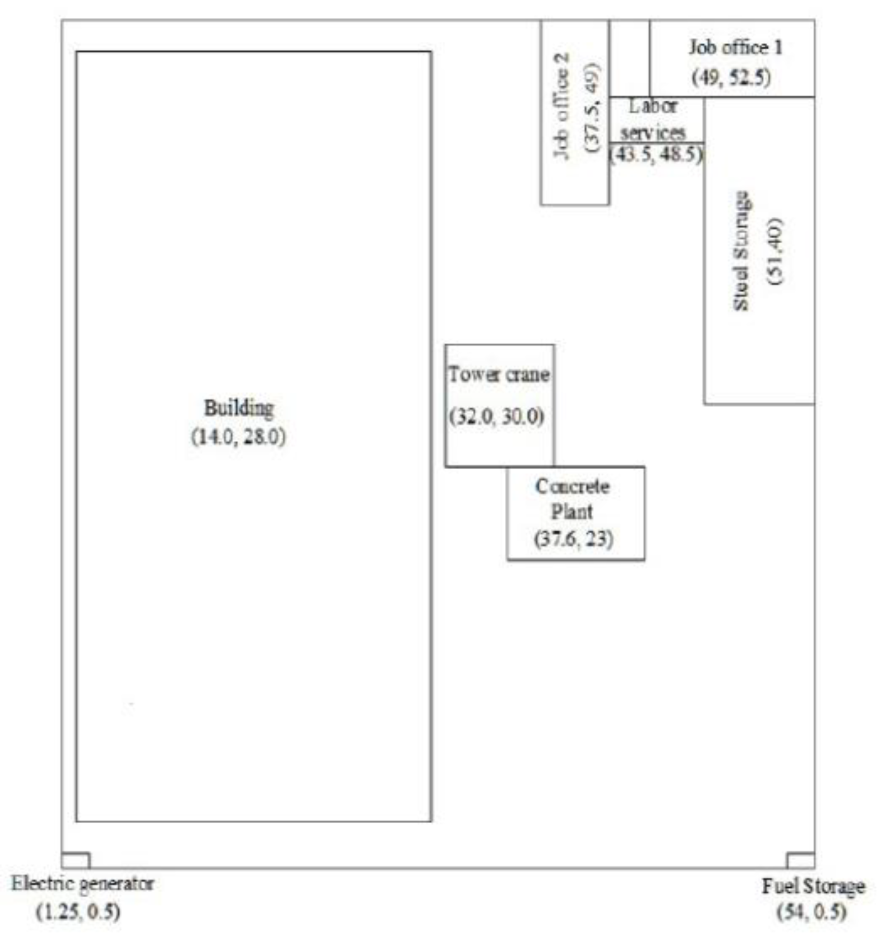
The optimization process was run several times to develop the optimal coordinates and probability of failure of each facility as well as the probability of failure of the whole site. The optimization solution provided a relative position between facilities. Figure 7 displays one possible layout and the results associated with it. It shows the location and optimized coordinates of each facility on a construction site. It is obvious that the hazardous facilities (F₁ and F₇) are allocated far away from all other facilities. Furthermore, this state is not applicable for facility F_9, since it was a fixed facility and its location was known in advance. Moreover, the facilities which were classified to be a high vulnerability (F₂, F₄, and F₅) are piled up far away from the fire hazard sources facilities. They are located at the top right of a construction site. This result coincides with the logical, intuitive expectation, since the failure of each facility was a convolution product of hazard and vulnerability, and the risk was a combined effect of the individual failures of all facilities. Therefore, this required accommodating the potential hazard sources’ facilities far away from the high vulnerability ones in order to minimize the total risk.

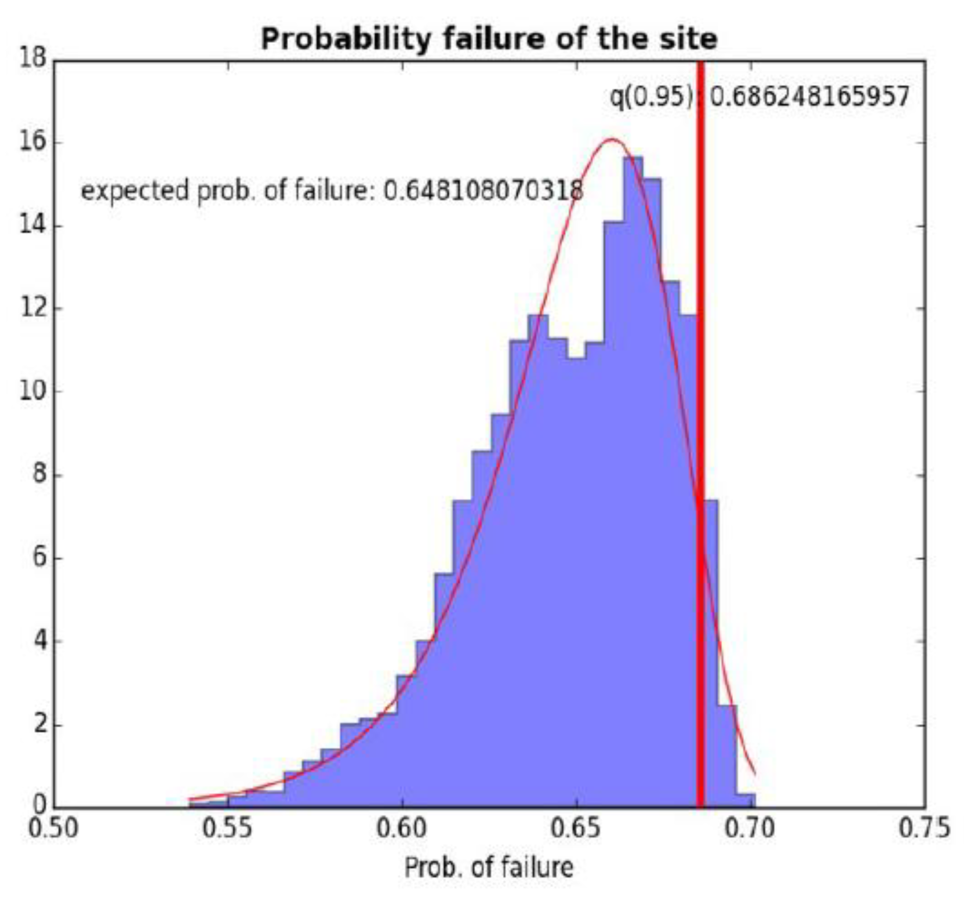
Figure 8 shows the uncertainty in the probability of failure of the whole site. It shows that with a 95% confidence level, the probability of failure of the whole site will not exceed 0.686. It shows also that the expected probability of failure of the whole site is 0.648. Moreover, the probability distribution of the failure of the whole site is skewed to the left (negative skewness) and tends to be a Weibull distribution function. On the other hand,

Table 3. Expected probability of failure for each facility and for the whole construction site.

Object	Expected Probability of Failure
F1	0.36561
F2	0.00099
F3	0.03728
F4	0.00013
F5	0.00304
F6	0.00139
F7	0.36311
F8	0.04295
F9	0.14375
Whole site	0.64811

presents the expected probability of failure of each facility as well as the whole site. It shows that the probabilities of failure of facilities (F₁ and F₇) were the highest, whereas the probability of failure of the facility (F₄) was the lowest due to its remoteness from all hazard sources. In general, the probability of failure of hazard source facilities was the highest. This can be attributed to the highest fire hazard intensity values at these facilities, so that these facilities were greatly governing the probability of failure of the whole site. The project managers must give them more attention during the execution phase of the construction project.

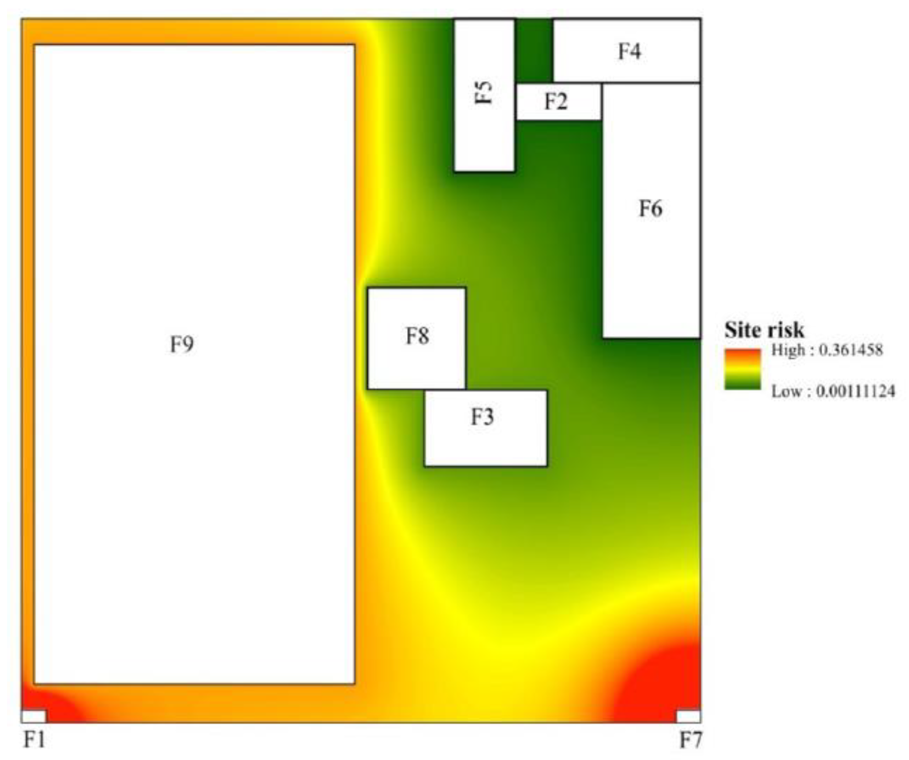
The interpolation technique available with the GIS is run on an optimal site layout, using the expected probability of failure of each facility, in order to develop a spatial fire risk map. Figure 9 confirms that the positions adjacent to facilities with a high probability of failure are more dangerous than those located far away from them. It is also clear that the top right of the construction site near facilities F₂, F₄, F₅, and F₆ corresponded to the safest places on a construction site, whereas the most dangerous positions (the riskiest) were located near facilities F₁ and F₇ at the bottom right and bottom left of the construction site. In addition, there was a moderate risk in the zones around the building under construction (F₉), which can be attributed to the moderate probability of failure of F₉.

5. Conclusions

In this paper, a probabilistic framework aimed to optimize construction site layouts by minimizing the probability of failure of the whole site due to fire. The framework relied on probabilistic and simplified physical modeling of hazard, vulnerability, and risk. The differential evolution algorithm was then run to start the optimization process. The GIS was utilized to develop the spatial fire risk map on a construction site. In the framework, it was assumed that the failure of the site would be a combined effect of independent individual failure of all facilities. The framework was carried out on a case study which consisted of several facilities, three of them considered potential hazard sources with different hazard levels. Furthermore, all of them were considered potential targets for a fire. The results showed that the model was efficient and easy to implement due to its ability to generate an optimal layout and display the riskiest positions on a construction site.

Even though the framework was efficient, there is still a need to enhance it by studying the physical characteristic of a fire hazard in depth and to develop more realistic hazard models. Furthermore, developing vulnerability curves for temporary facilities due to hazard is also another challenge. To validate the model and obtain the best parameters values of the probability density function, it is necessary to find a correlation between theoretical damage levels and actual ones considering different fire hazard intensity values. Finally, developing a dynamic site layout considering the purpose of the facility changes over time, conducting a trade-off analysis between risk and cost distance, and developing models dealing with irregular facilities as well as irregular construction sites are other potential future developments.