Article

Short-Term and Medium-Term Drought Forecasting Using Generalized Additive Models

1
Department of Hydrology and Water Resources, University of Venda, Thohoyandou 0950, South Africa
2
Department of Statistics, University of Venda, Thohoyandou 0950, South Africa
3
Unit for Environmental Sciences and Management, North-West University, Vanderbijlpark 1900, South Africa
*
Author to whom correspondence should be addressed.
Sustainability 2020, 12(10), 4006; https://doi.org/10.3390/su12104006
Submission received: 8 April 2020 / Revised: 6 May 2020 / Accepted: 7 May 2020 / Published: 14 May 2020

Abstract

:
Forecasting extreme hydrological events is critical for drought risk and efficient water resource management in semi-arid environments that are prone to natural hazards. This study aimed at forecasting drought conditions in a semi-arid region in north-eastern South Africa. The Standardized Precipitation Evaporation Index (SPEI) was used as a drought-quantifying parameter. Data for SPEI formulation for eight weather stations were obtained from South Africa Weather Services. Forecasting of the SPEI was achieved by using Generalized Additive Models (GAMs) at 1, 6, and 12 month timescales. Time series decomposition was done to reduce time series complexities, and variable selection was done using Lasso. Mild drought conditions were found to be more prevalent in the study area compared to other drought categories. Four models were developed to forecast drought in the Luvuvhu River Catchment (i.e., GAM, Ensemble Empirical Mode Decomposition (EEMD)-GAM, EEMD-Autoregressive Integrated Moving Average (ARIMA)-GAM, and Forecast Quantile Regression Averaging (fQRA)). At the first two timescales, fQRA forecasted the test data better than the other models, while GAMs were best at the 12 month timescale. Root Mean Square Error values of 0.0599, 0.2609, and 0.1809 were shown by fQRA and GAM at the 1, 6, and 12 month timescales, respectively. The study findings demonstrated the strength of GAMs in short- and medium-term drought forecasting.

1. Introduction

Rainfall variability is highly significant on several temporal and spatial scales in southern Africa [1,2,3,4], as most rural livelihoods in the region depend on agriculture, which is largely rainfed. Increasing trends of rainfall have been reported for a few locations over South Africa [5,6,7,8]. However, the authors of [9] cautioned that whilst this may suggest an increase in water resource availability, an increasing population and land use changes, coupled with intensification of agricultural activities, exert pressure on them. Although rainfall trends have been predicted to decrease in the Luvuvhu River Catchment (LRC) in the northeast of South Africa, some stations exhibited increasing trends, which were potentially attributed to the 10 year decadal mean daily fluctuations [10]. The chronic nature of drought disasters in the region further affects social, economic, and environmental aspects negatively [11]. The authors of [9] found an increasing trend of annual maximum temperatures in the Limpopo River Basin, which is consistent with several other land areas. Increased temperatures exacerbate drought characteristics (i.e., frequency, duration, and severity) [12], since there exists a positive linear relationship between increased temperature and evapotranspiration.
Prolonged droughts are a regular and recurrent feature of the southern African summer climate [13] and threaten vulnerable communities (most of whom are rural) of the region. About 60% of Sub-Saharan Africa is vulnerable to drought, with 30% being highly vulnerable [14]. The Southern Africa Development Community (SADC) region was struck by major droughts, notably in the years 1982/83, 1987/88, 1991/92, 1994/95 [15], and 2005/06 [9]. The authors of [16] further reported regular occurrences of drought in the LRC with a return period of 10 years, which ranged from 22.4% to 65% mild drought conditions. It was estimated that the 1991/92 drought resulted in 50,000 job losses in the agricultural sector in South Africa, which affected over 250,000 citizens [17].
More recently, the country experienced two consecutive droughts in 2014/2015 and 2015/2016, which resulted in severe water shortages in the Western Cape Province [18]. The Limpopo region, located in north-eastern South Africa, is prone to severe drought and flood events due to significant intra-seasonal variability during the core rainy season (December–February) [19,20]. Although the LRC has a substantial flow of water derived from the mountainous area at its source, during drought season, water resources become inadequate to meet the ecological reserve and domestic water supply [21].
Due to the increasing frequency and magnitude of drought events in the study area, area-specific forecasting has become of importance. Drought-index-based drought forecasting has been reported in northern areas of Pakistan and in Australia by [22,23], respectively. Forecasting and early warning of the drought phenomenon are increasingly being applied in many regions in the world. This is being done to mitigate the consequences of drought in vulnerable river basins. Although earth systems models to forecast drought have been developed over the years, these are large-scale models that are not area-specific. To adequately assess and manage drought risk in a catchment, finer-scale forecasting is important. This has potential to generate information on water resources that is useful to affected communities, including those whose livelihoods depend on rainfed agriculture.
Recent decades have seen the development of area-specific models applicable at finer scales. These models range from regression-based, probability, dynamical modeling, artificial neural networks, hybrids, etc. Two distinct studies [24,25] have carried out a detailed review of these drought forecasting models. Some of the common drought forecasting models include the autoregressive integrated moving average (ARIMA) [26] and its many variations, adaptive neuro-fuzzy inference system, Markov chain model [27], log-linear model, Empirical Mode Decomposition (EMD) [28], Empirical Wavelet Transform (EWT) [29], and Artificial Neural Network (ANN) [30] model, among others. Studies such as [23] successfully forecasted six-month lead time NADI (Non-linear Aggregated Drought Index) values for the Yara River Catchment in Australia, making use of ANN (DMSNN—Direct Multi Step Neural Network and RMSNN—Recursive Multi Step Neural Network). Generalized Additive Models (GAMs), however, have not been well documented in their capability and efficiency in forecasting drought conditions. This study, therefore, aims to forecast short- and medium-term drought conditions in the LRC using the Standardized Precipitation Evaporation Index (SPEI) as a drought-quantifying variable.

2. Materials and Methods

2.1. Case Study Description (LRC) and Datasets

The study area, the LRC, is located between latitudes 22°17′33.57″S and 23°17′57.31″S and longitudes 29°49′46.16″E and 31°23′32.02″E in Vhembe District of Limpopo Province in northeastern South Africa, as shown in Figure 1. The catchment covers an area of approximately 5941 km2 and is situated on a plateau about 1500 m above sea level. The catchment consists of a relatively rolling landscape, which gives rise to shallow storage dams that have large water surfaces exposed to evaporation. The topography of the catchment influences rainfall distribution with the highest rainfall received in the upper reaches (1800 mm/a), while the lower reaches around the Kruger National Park receive the lowest rainfall (400 mm/a) during the wet season. The catchment’s mean annual rainfall is 608 mm, and produces a mean annual run-off of 520 × 10 6 m 3 [10]. The distribution of rainfall through the year exhibits highly seasonal characteristics, with 95% of the rainfall occurring during the summer months (October and March) [31]. The lower-rainfall area in the catchment tends to experience greater variability than the higher-rainfall areas. Temperature generally increases from the mountains in the west to the lower reaches in the east of the catchment, with local towns, such as Thohoyandou, experiencing daily average temperatures of 33 °C in summer and 24 °C in winter [32]. The study area is predominantly rural, with a community that is highly dependent on rain-fed commercial and subsistence agriculture.
The regional climate within which the LRC is located ranges from tropical rain in the coastal plains of Mozambique to tropical dry savannah and tropical dry desert further inland, south of Zimbabwe [33]. The mean spatial pattern of summer rainfall over southern Africa depicts a strong gradient that increases from west to east [34], with local maxima due to orographic effects. The LRC is a sub-basin of the Limpopo River Basin, in which annual precipitation varies between 250 to 1050 mm in the hot, dry western and central areas in the high-rainfall eastern escarpment areas, respectively [33]. The region experiences a high variability between extreme wet and dry seasons, which makes it vulnerable to frequent droughts and floods [35].
The nature and pattern of inter-annual variability of precipitation is crucial, as it exerts long-term control on water resources and affects plant growth and the bio-geochemical cycle while moderating extreme events such as droughts and floods [36]. The Limpopo valley (20–25 °S) is characterized by the highest variability in southern Africa [34], in agreement with [37,38]. Figure 2 and Figure 3 show the inter-annual variability of rainfall and streamflow in the LRC for over 57 and 53 years, respectively. The inter-annual variability plots depict a strong seasonal variation in the study area. The rainy season of the region is characterized by alternating wet and dry spells [39], with wet spells recently becoming shorter. Both rainfall and streamflow exhibit positive trends over the sampling periods considered although neither was statistically significant; rainfall showed an R2 of 0.0011, while streamflow reported 0.0043. These trend results agree with those obtained by [34] over southern Africa. Statistical trends in this region are affected by extremes, such as the significant flood due to tropical Eline in February 2000 (Figure 2 and Figure 3). From both Figure 2 and Figure 3, the trend equations are y = 0.0005 x + 86.734 and y = 0.0005 x + 53.446 , respectively. This means that both rainfall and streamflow increase at the rate of 0.0005 mm and 0.0005 cumesc per year. This intercept is made using the trendline gradient of the two variables.
Rainfall and temperature data from eight weather stations were obtained from the South African Weather Service, while evaporation data for one station were obtained from the Department of Water and Sanitation within the Luvuvhu River Catchment. The location of all the stations is shown in Figure 1 and additional details are shown in Table 1. These datasets were obtained from 1986 to 2016, covering 31 years. The missing data in this study were imputed using the Self-Organizing Maps (SOM) based on the Kohonen Neural Networks [40].

2.2. Formulation of the SPEI for the Study Area

The SPEI is based on the computation procedure of the original SPI (Standardized Precipitation Index). The index makes use of either monthly or weekly differences between precipitation and Potential Evapotranspiration (PET) [41]. Due to the complex computation of PET, which involves several variables, including surface temperature, air humidity, soil, incoming radiation, water vapor pressure, and ground–atmosphere latent and sensible heat fluxes [42], this study made use of Hagreaves’ and Samani’s temperature-based method for PET estimation. This approach has the advantage of only requiring data on monthly mean temperature. The SPI methodology was modified by replacing the two-parameter distribution with a three-parameter distribution (i.e., SPEI requirement) [41]. The latter suggested getting the best fit three-parameter distribution from the L-moment, and the detailed methodology for achieving this can be obtained in [43]. Following the classical approximation of [44], the SPEI for this study was formulated at 1, 6, and 12 month timescales using Equation (1).
S P E I = W C 0 + C 1 W + C W 2 2 1 + d 1 W + d 2 W 2 + d 3 W 3
where W = 2 ln ( P ) for P 0.5 , and P is the probability of exceeding a threshold value denoted by D value, P = 1 F ( x ) . If P > 0.5 , then P is replaced by 1 P and the sign of the resultant SPEI is reversed. The constants C0, C1, C2, d1, d2, and d3, are 2.515517, 0.802853, 0.010328, 1.432788, 0.189269, and 0.001308 as defined by [45], respectively. For this study, the SPEI was computed using the R Package “spei” developed by Begueria [46].

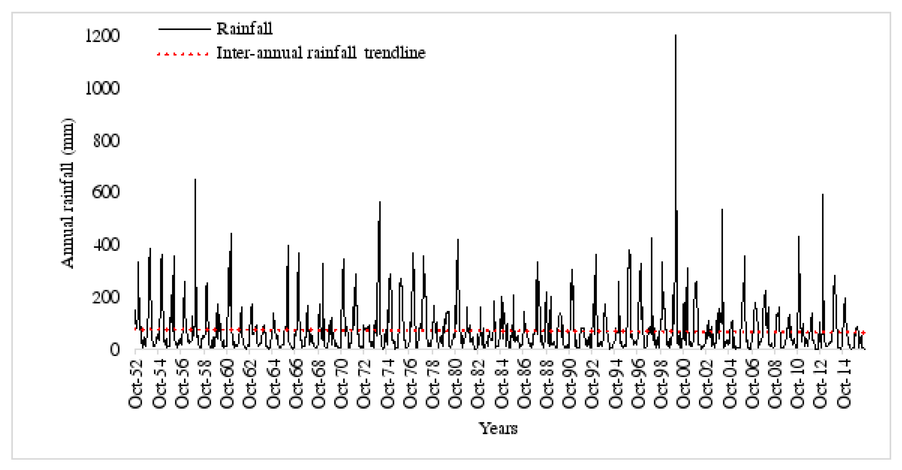
2.3. Drought Trends over North-Eastern South Africa

The Breaks for Additive Seasonal and Trend (BFAST) method in Equation (2) is applied to decompose the drought index time series to obtain the trend variations in the study area.
y t = m + T t + S t + R t
where m is the mean, T t is the trend component value, S t is the seasonal component, and R t is the random component at time t . The monotonic trends in the SPEI time series were obtained through the Mann–Kendall (MK) non-parametric trend test. Based on studies by [47,48,49,50,51], among others, the MK test statistic is calculated from the following formula:
S = k = 1 n 1 j = k + 1 n s i g n ( X j X k )
s i g n ( x ) = { 1 0 1 x j > x i x j = x i x j < x i
The average value of S is E[S] = 0 and the variance σ 2 is given by the following equation:
σ 2 = { n ( ( n 1 ) ( 2 n 5 ) i = 1 p t j ( t j 1 ) ( 2 t j + 5 ) } 18
where t j is the number of data points in the j t h tied group, and p is the number of the tied group in the time series. It is important to mention that the summation operator in Equation (5) is applied only in the case of tied groups in the time series to reduce the influence of individual values in tied groups in the ranked statistics. On the assumption of random and independent time series, the statistic S is approximately normally distributed if the following z-transformation equation is used. The value of the S statistic is associated with the Kendall tau, as shown in Equation (7).
Z = { S 1 σ 0 S + 1 σ S > 0 S = 0 S < 0
τ = S D
where
D = [ 1 2 n ( n 1 ) 1 2 j 1 p t j ( t j 1 ) ] 1 2 [ 1 2 n ( n 1 ) ] 1 2
With regards to the z-transformation equation in Equation (6), this study considered a 5% confidence level, where the null hypothesis of no trend was rejected if |z| > 1.96. The Mann–Kendall statistic is the Kendall τ term, which is a measure of correlation that indicates the strength of the relationship between any two independent variables, and was also considered important in this study. The MK test system summarized above was applied to the SPEI time series data by writing a code in R and following the instructions given by [52].

2.4. SPEI Time Series Forecasting

The forecasting procedure followed in this study started with selecting important variables, formulation of training and testing sets, and determination of model performance. The training data consisted of 70%, while the testing sets were 30% of the total data. The developed models’ test sets were based on the correlation coefficient (R), Root Mean Square Error (RMSE), Mean Error (ME), Mean Absolute Error (MAE), Mean Percentage Error (MPE), and the Mean Absolute Percentage Error (MAPE). The forecasting of SPEI at 1, 6, and 12 month timescales using GAM is discussed below.

2.4.1. The Generalized Additive Model without Auto-Correlated Errors

Let y t be the SPEI on month t , where t = 1 , , n with the corresponding covariates x t 1 , x t 2 , , x t p , where p represents the number of variables. The generalized additive model is then written as follows:
y t = β 0 + j = 1 p s j ( X t β j ) + ε t
where y t is the response variable, X t is a matric of covariates, β 0 is the intercept, β j are parameters, s j is a smoothing parameter, and ε t is the error term. It should be noted that, although y t denotes the SPEI at month t , it was used to for all the timescales considered in this study. Equation (9) is estimated using penalized cubic splines [53,54], which is expressed in terms of Equation (10). This should be:
min s j [ t = 1 n ( y t β 0 j = 1 p s j ( X t j ) ) 2 + j = 1 p λ j ( ( f ( x ) ) 2 d x ) ]
The degree of smoothness is controlled by the penalty parameter Λ = ( λ j , j = 1 , , p ) , which determines the roughness of the function estimate to the data. It is optimized using the generalized cross-validation criterion (GCV) and is easily implemented in the package ‘mgcv’ [53,55]. For small values of λ j , the smoothness is rough. The smooth function, s j , is given by Equation (11), which can be explained as the sum of the basis functions b i ( x ) and their regression coefficients β i .
s j ( x ) = i = 1 q β i b i ( x )
where q denotes the basis dimension.

2.4.2. The Generalized Additive Model with Auto-Correlated Errors

Let y t be the SPEI as defined in Section 2.4.1, which gives the generalized additive model in Equations (12), where the error terms ε t are assumed to be autocorrelated.
y t = β 0 + j = 1 p s j ( X t β j ) + ε t
where variables and parameters are as defined above. Time series observations are normally autocorrelated. To correct for autocorrelation, it is normally advised to use time series regression models. This study, therefore, assumes that the error terms ε t are auto-correlated and follow the SARIMA model given in Equation (13).
θ ( B ) Φ ( B ) ε t = θ ( B ) Θ ( B ) v t
where θ ( B ) is the non-seasonal moving average operator, and the corresponding seasonal autoregressive and seasonal moving operators are Φ ( B ) and Θ ( B ) , respectively; v t denotes a white noise series. By expressing Equation (12) in terms of ε t and substituting in Equation (13), we get Equation (14).
θ ( B ) Φ ( B ) [ y t { β 0 + i = 1 p s j ( X t β j ) } ] = θ ( B ) Θ ( B ) v t

3. Results

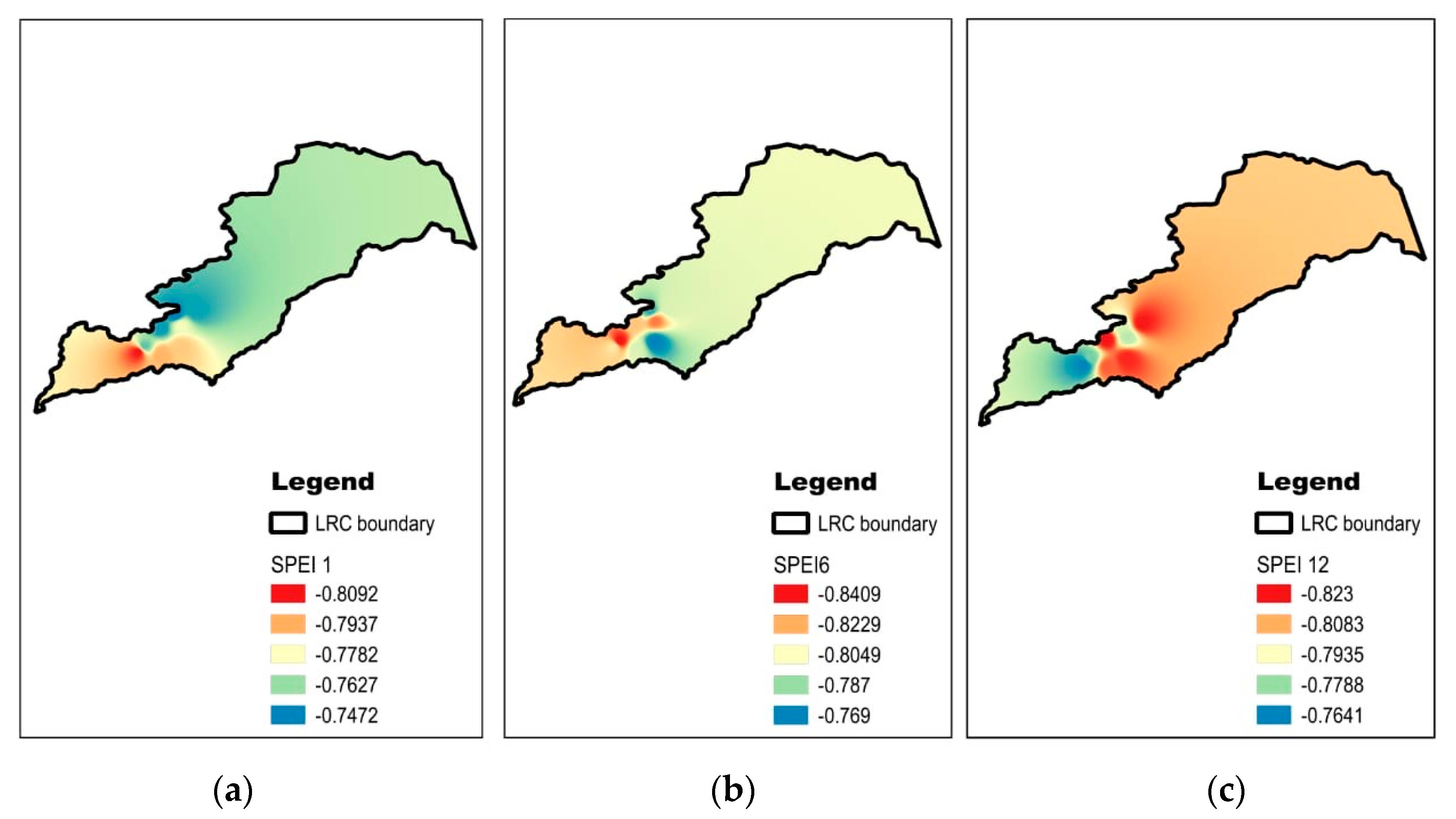
3.1. Spatial Variability of Drought in the Study Area

Table 2 shows the different drought categories in terms of percentages of occurrence of historical drought for all the stations at different timescales. Mild, moderate, severe, and extreme droughts conditions ranged between 61.15–71.88%, 12.65–27.59%, 2.24–21.69%, and 0–6.65%, respectively, across all stations and considering the respective timescales considered in the study. This shows that mild drought is more prevalent in the LRC compared to other drought categories. Stations Muk and Mat showed the highest percentages of extreme droughts (i.e., 6.14%) at one- and six-month timescales, while the Vondo Bos (VB) station showed the same with 6.65% at the 12 month timescale. However, this is still lower than the percentage of extreme events shown by the SPI at the same timescale. The spatial variability of the SPEI at 1, 6, and 12 month timescales is presented in Figure 4. The variability shows that SPEI 12 was found to be of greater severity compared to the one- and six-month timescales in the middle reaches, while, in the upper reaches, the 12 month timescale showed the least drought severity compared to the SPEI for one and six months.

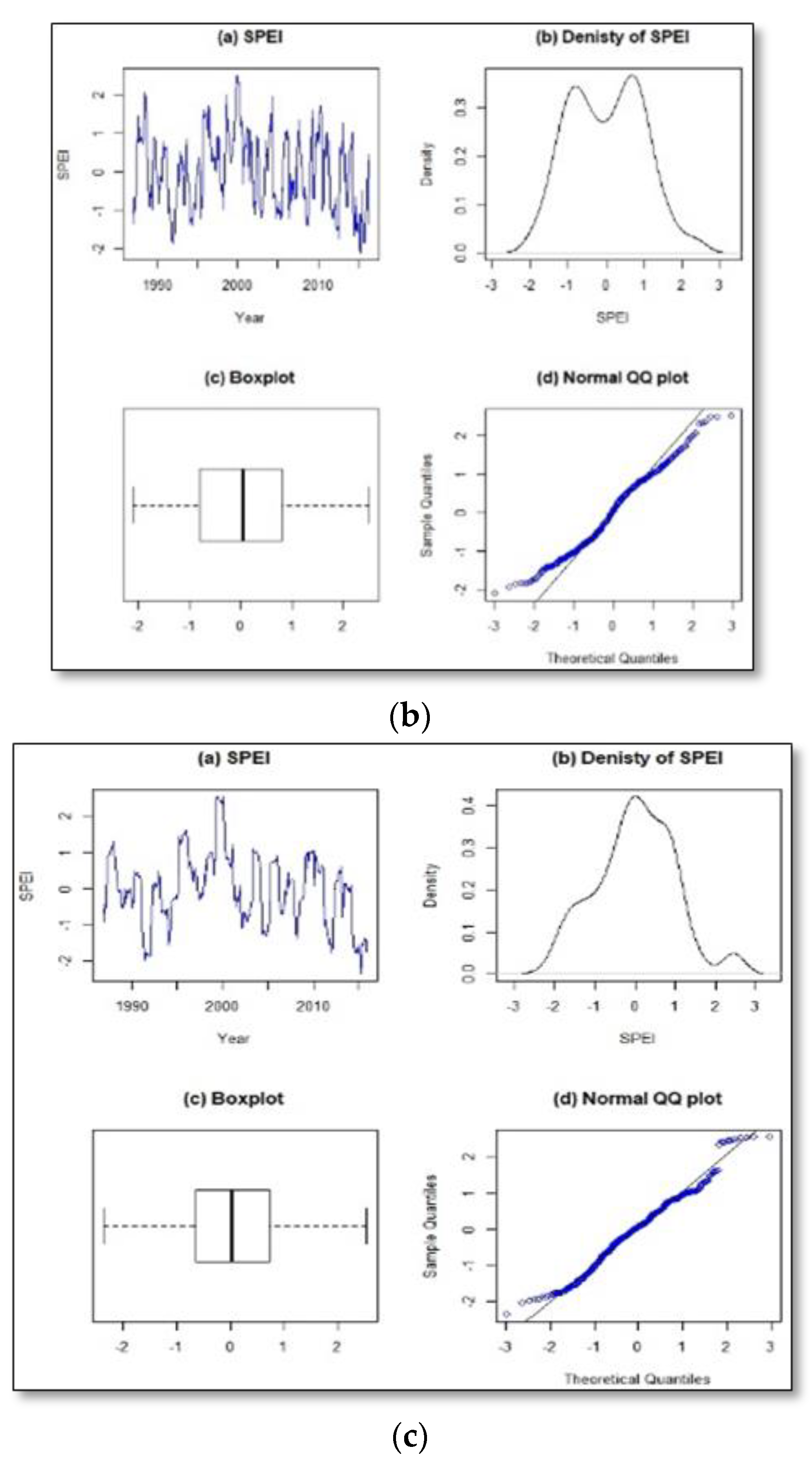
3.2. Exploratory Data Analysis

Figure 5 shows the SPEI time series plot of density, normal quantile to quantile (QQ), and the box plots at the 1, 6, and 12 month timescales before decomposition. To determine the normality of the SPEI data, the Anderson–Darling test was carried out. The initial visual interpretation of the QQ plot suggested departure from the normality of SPEI data, while the detailed Anderson–Darling test Probability–Probability Plot (PP) showed that the data are approximately normally distributed at all the timescales. The authors of [56,57] reported that although visual inspection of normality is used, it is often unreliable, with no guarantees of the results. Johnson SB, Error, and Dagun (4P) distributions were the best fit for the SPEI 1, 6, and 12 month timescales, respectively. From this, the study concluded that the distributions of the SPEI data at 6 and 12 month timescales are bimodal, while the one-month timescale exhibited a unimodal distribution.

3.3. Variable Selection

Variable selection was achieved using gradient boosting. The main objective of a variable selection procedure is to identify the correct predictor variables, which have important influence on the response variable and could provide robust model prediction [58]. Variable selection was conducted for each SPEI time series. The relative importance values are the means of 50 model runs, each based on a randomly selected subset of 90% of the data [59]. Rain showed to be the most important variable for predicting the SPEI at the one-month timescale, while the non-linear trend is the most important predictor for predicting the SPEI at the six-month timescale. Time series components (i.e., trend, seasonality, remainder, etc.) have been successfully used as model inputs in forecasting exercises. For example, the authors of [60] used time series components in forecasting airline passengers using ANN. The authors of [61] reported three significant consecutive lags (i.e., Lags 1, 2, and 3) as input while predicting daily PM10 data. The lagged variable of importance was successfully determined by Principal Component Analysis (PCA). The findings of this study regarding the importance of Lags 1 and 2 are therefore comparable with those reported by [61]. Temperature, which plays a significant role in the development of drought through influence on evaporation, was found to be important in the SPEI at the one- and six-month timescales. The authors of [62] reported that sea surface temperature variability contributed to increased land temperature variability and autocorrelation, which ultimately contributed to persistent droughts in North America and the Mediterranean. Mean temperatures were noted to be more dominant compared to the minimum and maximum temperatures in forecasting the SPEI. All predictor variables are significantly different from one another in their relative importance [59]; therefore, all features that appeared to have some relative importance (i.e., ranging from 0 to 100) were selected as input variables in forecasting drought over the LRC and are presented in Table 3.

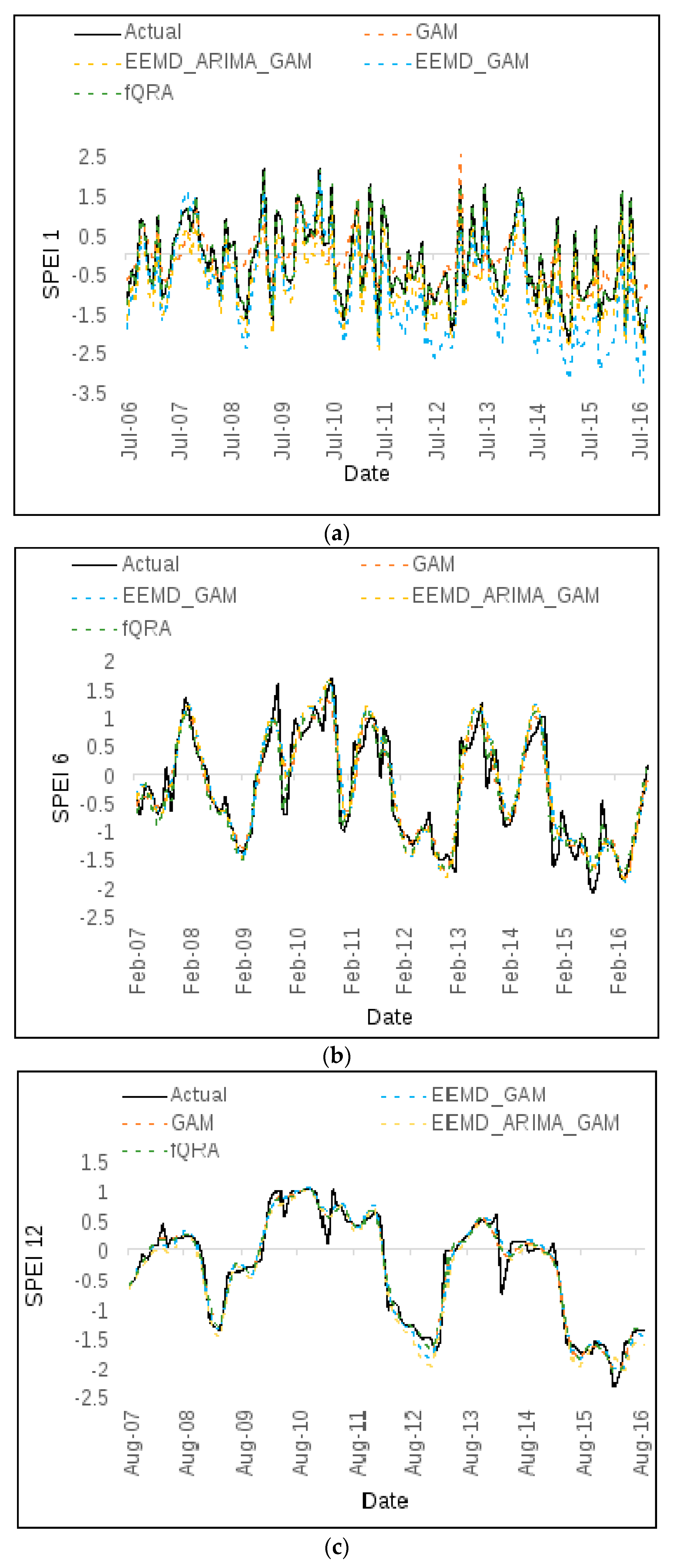
3.4. Short- and Medium-Term Forecasting

To understand the forecasting performance of statistical models, a comparative study was conducted between the four developed models. Figure 6 shows the models’ drought forecasting results at all timescales considered in this study. The smoothing effect of the GAM models is evident in the forecasting results. The GAM provides a flexible specification of response by defining the model in terms of smooth functions as a replacement for the detailed parametric relationships on the covariates [63]. The decomposition of environmental time series is expected to improve the forecasting accuracy of models, and it is evident at all timescales that the decomposed GAM performed better than an undecomposed GAM. Although an Ensemble Empirical Mode Decomposition (EEMD)-GAM forecasted the SPEI better than the GAM, from Figure 6, the EEMD-GAM is seen to overestimate drought conditions, especially between 2011 and 2016, with the GAM greatly underestimating the target values, while the EEMD-ARIMA-GAM (i.e., the GAM after correcting residual autocorrelation) improved the forecast. This was noted clearly in the one-month timescale, while for the 6 and 12 month timescales, all models showed some level of improvements. The results of this study agree with those of [64], which found that incorporating corrected residual autocorrelation increased model performance and improved the out-of-sample forecasts. Since forecasting models are imperfect abstracts of reality [65], such behaviors in model outputs are therefore expected, as the forecasts are often not perfect.

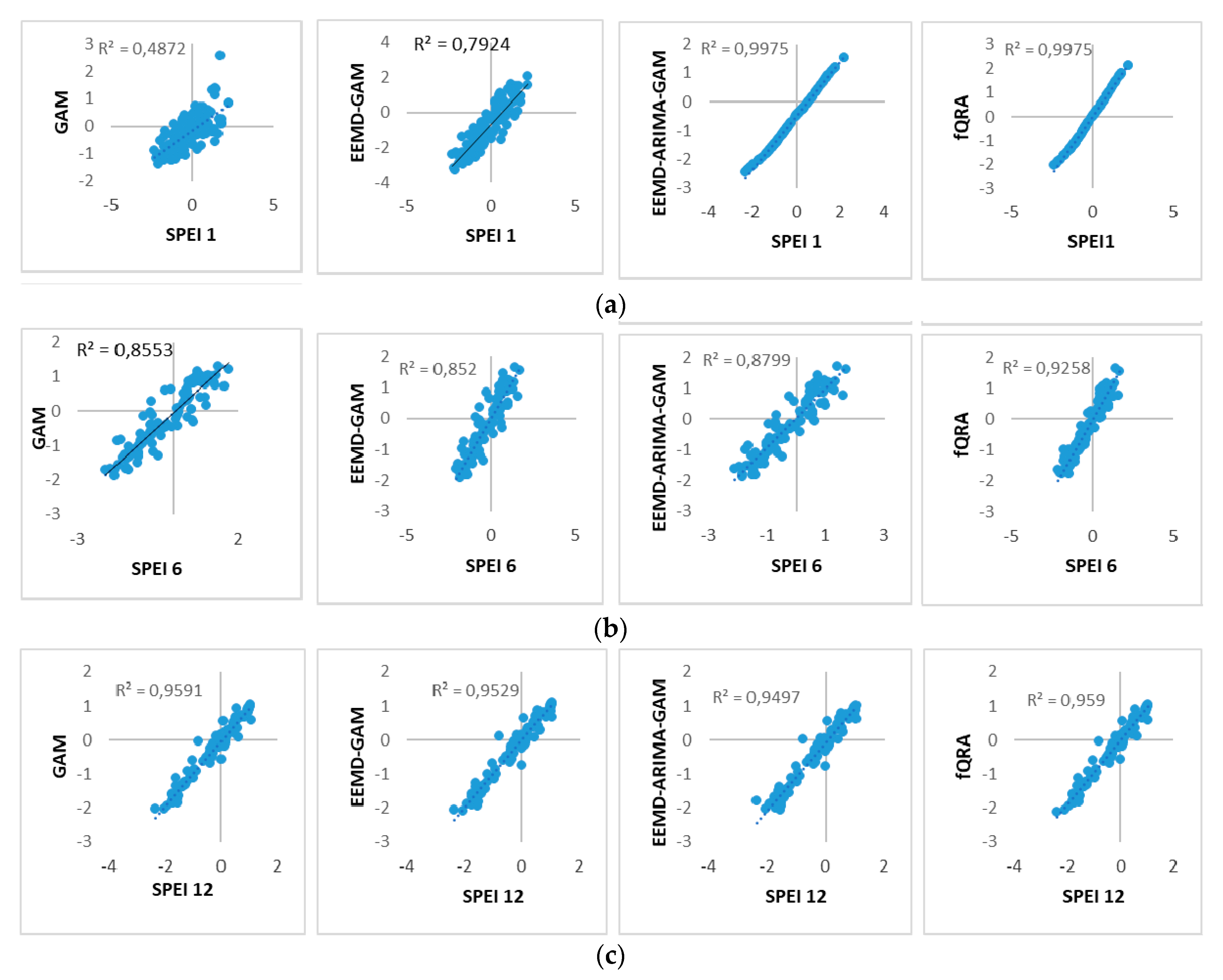
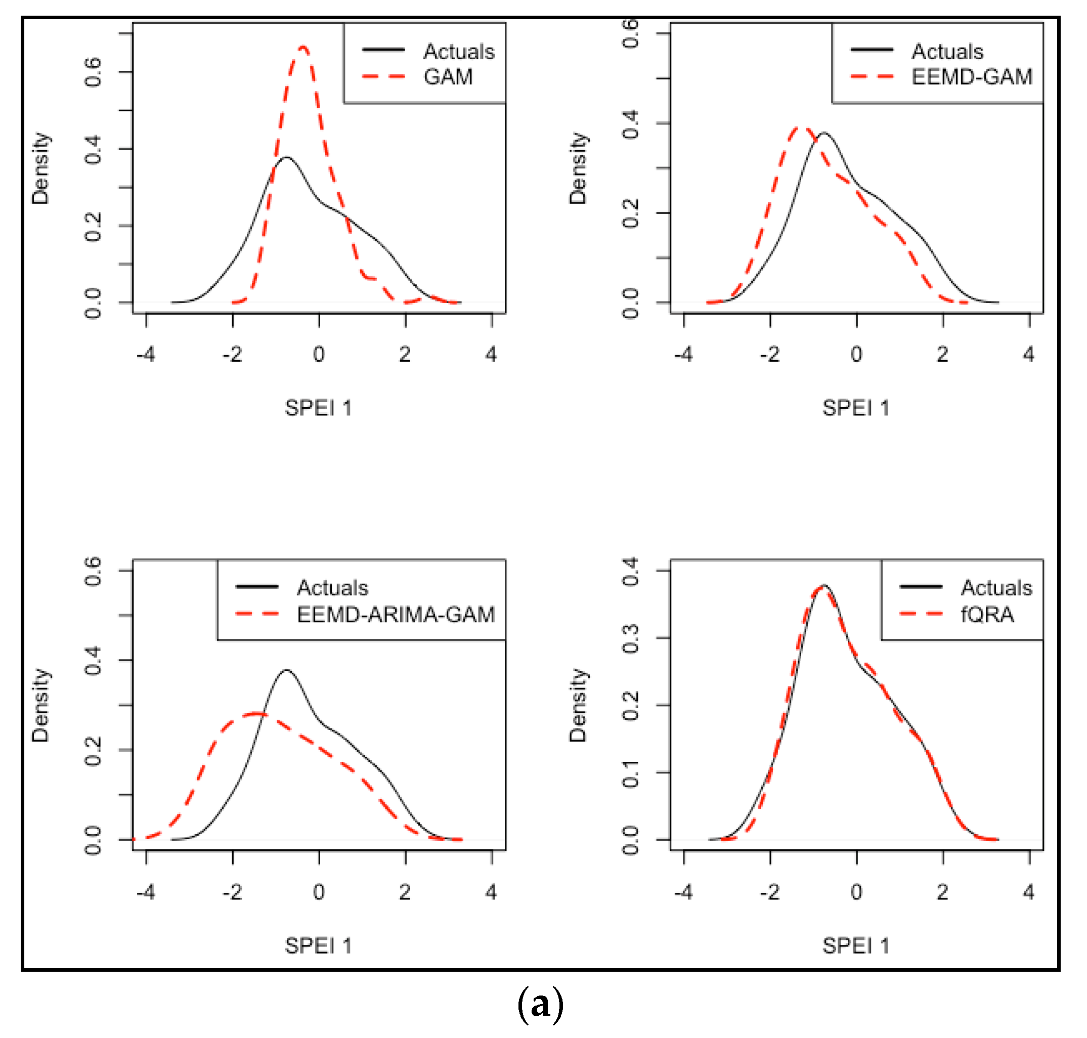
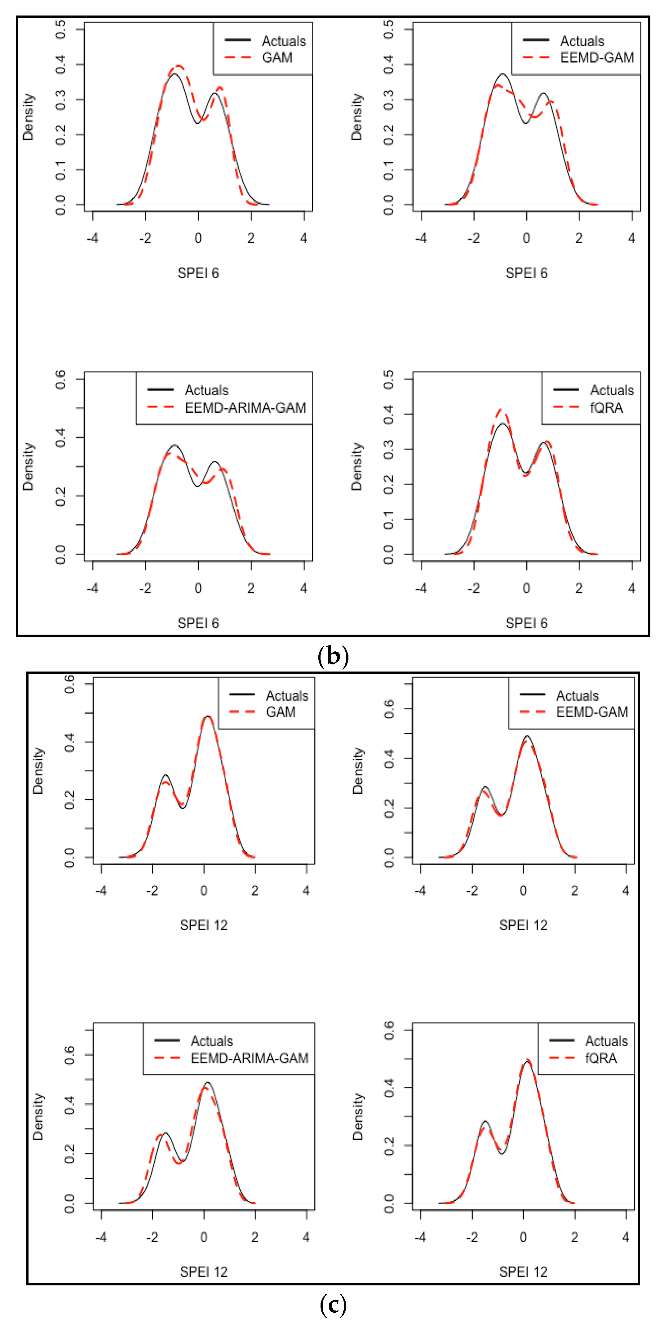
3.5. Model Performance

Figure 7 is the scatterplot of the different models’ outputs at all the timescales considered in this study. All the models’ results show that a positive correlation exists between the modeled output and the actual data. The GAM, EEMD-GAM, and EEMD-ARIMA-GAM forecast results showed the lowest correlation at the 1, 6, and 12 month timescales, respectively. The fQRA showed the highest correlations at the one- and six-month timescales, while, for the 12 month timescale, the GAM showed the highest correlation. The high correlation showed by fQRA may be because fQRA is made up of a weighted combination of all the models; therefore, all the models’ strength results in fQRA are superior compared to the other models developed in this study. In addition to the correlation between the forecasted and target values, this study employed further statistical measures to determine the model performance, and these are shown in Table 4. The best RMSE was shown by fQRA at the one- and six-month timescales, with the 12 month timescale showing that the GAM performed better compared to the other models. The incorporation of autocorrelation errors as reported by [64] is noted in the model performance at the one- and six-month timescales. These models were seen to have performed better than the GAM and decomposed GAM at the one- and six-month timescales, therefore showing that decomposition coupled with autocorrelation errors improves forecasting accuracy.
The density plots from all the developed models (i.e., GAM, EEMD-GAM, EEMD-ARIMA-GAM, and fQRA) at the three timescales superimposed with actual SPEI time series are given in Figure 8a–c. Similar to the results shown by the different model performance measures, at the one- (Figure 8a) and six-month (Figure 8b) timescales, the fQRA models showed fairly good density fits compared to the other models. At the 12 month timescale, both the GAM and fQRA showed good density fits, and the same was noted by the different performance measures.

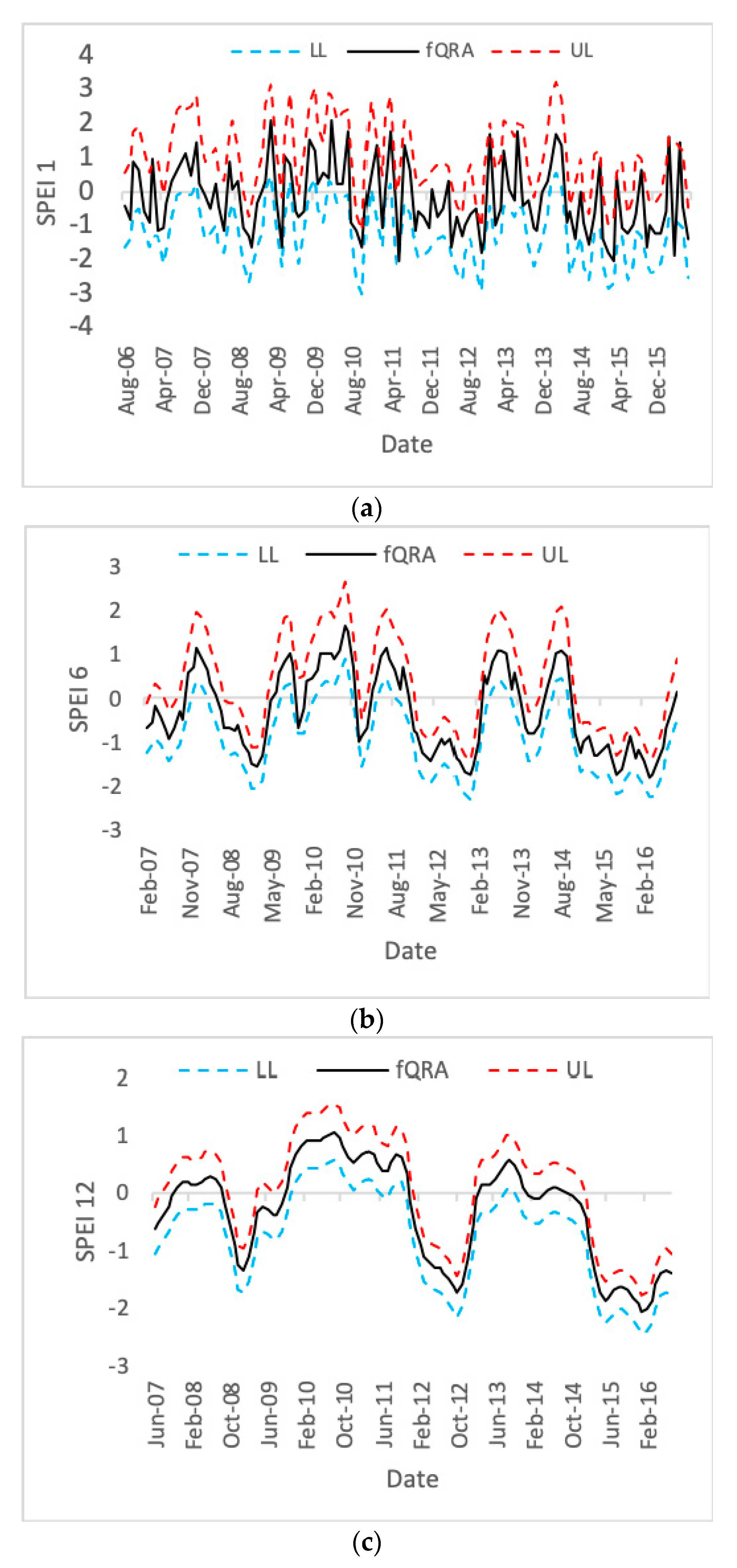
3.6. Evaluation of Model Uncertainity

Uncertainty analysis in this study was carried out only for the best performing statistical GAM-based models. This was achieved by constructing empirical prediction intervals (PIs) at all timescales. Figure 9 shows the 95% prediction limits of the GAM-based models. The skewness at the one- and six-month timescales was positive, while the 12 month timescale showed a negative skewness. At the 12 month timescale, the model showed the smallest standard deviation, which is indicative of a narrower prediction interval.
El Niño conditions alter moisture flux circulation over southern Africa, thereby influencing the spatial pattern and intensity of drought over the region [66]. The authors of [67] found that it was possible to forecast El Niño events approximately one year ahead, as well as the highest peak based on the characteristics of a previous event. Uncertainty of climatic variables in the future due to climate change is a reality, which ultimately influences drought patterns. Although the models in this study were developed based on historical data, with the availability of downscaled future rainfall and temperature, the developed models can be tested for the uncertainty of future drought patterns.

4. Discussion

With the increasing frequency and magnitude of extreme hydrological events over the Limpopo River Basin, studies that seek to evaluate the likelihood of these events occurring in the future are important. Since water resources are the core of human existence and environmental health, reliable early warning systems have become important. This study used SPEI time series as a drought-quantifying parameter to describe drought conditions at short- and medium-term timescales (one- and six-month timescales are short-term, while a 12 month timescale is medium-term in this study). To reduce the inherent complexities of hydrological data, time series decomposition was conducted and correction of autocorrelated errors was done as well as forecast combination to improve the forecasting accuracy of the developed models. Mild droughts were found to be the most dominant in the study area compared to severe and extreme drought conditions.
The variability shows that SPEI 12 has greater severity compared to the one- and six-month timescales in the middle reaches, while, in the upper reaches, the 12 month timescale showed the least drought severity compared to SPEI one- and six-months. Four models (GAM, EEMD-GAM, EEMD-ARIMA-GAM, and fQRA) were developed to forecast drought in the LRC at short- and medium-term timescales. The study found that correction of autocorrelated errors and decomposition improved model performance. At the one- and six-month timescales, the fQRA performed better, followed by EEMD-ARIMA-GAM, while the 12 month timescale behaved differently. This timescale showed that the GAM was better than the decomposition with and without corrected autocorrelated errors. An RMSE difference of 0.002% was noted between the GAM and fQRA at this timescale, making these two models the best at this timescale.

5. Conclusions

This study aimed to characterise drought and evaluate the performance of GAM-based models in drought forecasting in a semi-arid catchment at short and medium terms. Although earth systems models are available for such exercises, these models often provide forecasts gridded over large areas without providing details for small catchments, such as the LRC. This makes studies of this nature important, as they focus on smaller scales where impacts on communities are measurable. The study showed the forecasting strength of GAM-based models for drought at short-term scales and further proved the hypothesis that decomposition and correction of autocorrelation errors together with time series decomposition improved model performance. For medium-term forecasting, this study found that the treatment of a time series did slightly improve the forecast, but an undecomposed GAM showed better performance at this timescale. These models showed their strength for short- and medium-term forecasting and can, therefore, be used for timely water resource decision-making in semi-arid regions. Thus, the forecast would serve as a decision support tool that would ensure advance knowledge of water resource availability and facilitate realistic planning and allocation to meet the minimum water requirements during drought periods, thereby reducing communities’ vulnerability to drought impacts. These models can, therefore, be incorporated into early warning systems in these regions to aid in better planning and management of water resources and drought risk reduction in the short and medium terms.

Author Contributions

The results of this study were obtained from a submitted PhD thesis at the University of Venda. Conceptualization, F.M.; methodology, F.M.; software, F.M. and C.S.; validation, F.M. and C.S.; formal analysis F.M. and C.S.; original draft preparation, F.M.; writing—review and editing, F.M., C.S., H.C., and J.O.; supervision, C.S., H.C., and J.O. All authors have read and agreed to the submitted version of the manuscript.

Funding

This research received no external funding.

Acknowledgments

The authors also acknowledge the Dean of the School of Environmental Sciences (University of Venda) for organizing the writing workshop that assisted in the reshaping of this paper.

Conflicts of Interest

The authors declare no conflict of interest.

References

  1. Tyson, P.D. Climatic Change Variability in Southern Africa; Oxford University Press: Cape Town, South Africa, 1986; p. 220. [Google Scholar]
  2. Nicholson, S.E.; Entekhabi, D. Rainfall variability in equatorial and southern Africa: Relationship with seas surface temperatures along the southwestern coast of Africa. J. Clim. Appl. Meteorol. 1987, 26, 561–578. [Google Scholar] [CrossRef] [Green Version]
  3. Fauchereau, N.; Trzaska1, S.; Rouault, M.; Richard, Y. Rainfall Variability and Changes in Southern Africa during the 20th Century in the Global Warming Context. Nat. Hazards 2003, 29, 139–154. [Google Scholar] [CrossRef]
  4. Ambrosino, C.; Chandler, R.E.; Tod, M.C. Southern African Monthly Rainfall Variability: An Analysis Based on Generalized Linear Models. J. Clim. 2011, 24, 4600–4617. [Google Scholar] [CrossRef]
  5. Mason, S.J.; Waylen, P.R.; Mimmack, G.M.; Rajaratnam, B.; Harrison, J.M. Changes in Extreme Rainfall Events in South Africa. Clim. Chang. 1999, 41, 249–257. [Google Scholar] [CrossRef]
  6. Easterling, D.R.; Meehl, G.A.; Parmesan, C.; Changnon, S.A.; Karl, T.R.; Mearns, L.O. Climate Extremes: Observation, Modeling and Impacts. Science 2000, 289, 2068–2074. [Google Scholar] [CrossRef] [PubMed] [Green Version]
  7. New, M.; Hewitson, B.; Stephenson, D.B.; Tsiga, A.; Kruger, A.; Manhique, A.; Gomez, B.; Coelho, C.A.S.; Masisi, D.N.; Kululanga, E.; et al. Evidence of trends in daily climate extremes over southern and west Africa. J. Geophys. Res. 2006, 111, D14102. [Google Scholar] [CrossRef]
  8. Kruger, A.C.; Nxumalo, M.P. Historical rainfall trends in South Africa: 1921–2015. Water SA 2017, 43, 285–297. [Google Scholar] [CrossRef] [Green Version]
  9. Mosase, E.; Ahlablame, L. Rainfall and temperature in Limpopo River Basin, southern Africa: Means, variation and trends from 1979 to 2015. Water 2018, 10, 364. [Google Scholar] [CrossRef] [Green Version]
  10. Odiyo, J.O.; Makungo, R.; Nkuna, T.R. Long-term changes and variability in rainfall and streamflow in Luvuvhu River Catchment, South Africa. S. Afr. J. Sci. 2015, 111, 1–9. [Google Scholar] [CrossRef]
  11. Gommes, R. Non-parametric crop yeild forecasting. A didactic case study for Zimbabwe. In Proceedings of the ISPRS Archives XXXVI-8/W48 Workshop proceedings: Remote sensing support to crop yield forecast and area estimates, Stresa, Italy, 30 November–1 December 2006; pp. 79–84. [Google Scholar]
  12. Vicente-Serrano, S.M.; Chura, O.; Lopez-Moreno, J.I.; Azorin-Molina, C.; Sanchez-Lorenzo, A.; Aguilar, E.; Moran-Tejeda, E.; Trujillo, F.; Martinez, R.; Nieto, J.J. Spatio-temporal variability of droughts in Bolivia. Int. J. Clim. 2014, 35, 3024–3040. [Google Scholar] [CrossRef] [Green Version]
  13. Rouault, M.; Richard, Y. Intensity and spatial extent of droughts in southern Africa. Geophys. Res. Lett. 2005, 32, L15702. [Google Scholar] [CrossRef]
  14. Benson, C.; Clay, E. The Impact of Drought on Sub-Saharan African Economies: A Preliminary Examination; Technical Paper No. 401; World Bank: Washington, DC, USA, 1998. [Google Scholar]
  15. FAO. Drought Impact Mitigation and Prevention in the Limpopo River Basin: A Situation Analysis; Food and Agricultural Organisation: Rome, Italy, 2004; p. 160. [Google Scholar]
  16. Odiyo, J.; Mathivha, F.I.; Nkuna, T.R.; Makungo, R. Hydrological hazards in Vhembe district in Limpopo Province, South Africa. Jàmbá J. Disaster Risk Stud. 2019, 11, 698. [Google Scholar] [CrossRef] [PubMed]
  17. Association for Rural Advancement (AFRA). Drought Relief and Rural Communities; Special Rep. No. 9; AFRA: Pietermaritzburg, South Africa, 1993. [Google Scholar]
  18. Department of Environmental Affairs (DEA). South Africa’s 2nd Annual Climate Change Report; DEA: Pretoria, South Africa, 2016.
  19. Levey, K.M.; Jury, M.R. Composite interseasonal oscillation of convection over southern Africa. J. Clim. 1996, 9, 1910–1920. [Google Scholar] [CrossRef] [Green Version]
  20. Cook, C.; Reason, C.; Hewitson, B. Wet and dry spells within particularly wet and dry summers in the South African summer rainfall region. Clim. Res. 2004, 26, 17–31. [Google Scholar]
  21. Department of Water Affairs and Forestry (DWAF). Luvuvhu/Letaba Water Management Area: Internal Strategic Perspective; DWAF Report No.P WMA 02/000/00/0304; DWAF: Pretoria, South Africa, 2004.
  22. Ali, Z.; Hussain, I.; Faisal, M.; Nazir, H.M.; Hussain, T.; Shad, M.Y.; Shoukry, A.M.; Gani, S.H. Forecasting Drought Using Multilayer Perceptron Artificial Neural Network Model. Adv. Meteorol. 2017, 5681308. [Google Scholar] [CrossRef]
  23. Barua, S.; Ng, A.W.M.; Perera, B.J.C. Drought assessment and forecasting: A case study on the Yarra River catchment in Victoria, Australia. Aust. J. Water Resour. 2012, 15, 95–108. [Google Scholar] [CrossRef]
  24. Mishra, A.K.; Singh, V.P. A Review of Drought Concepts. J. Hydrol. 2010, 391, 202–216. [Google Scholar] [CrossRef]
  25. Fung, K.F.; Huang, Y.F.; Koo, C.H.; Soh, Y.W. Drought forecasting: A review of modelling approaches 2007–2017. J. Water Clim. Chang. 2019, 1–29. [Google Scholar] [CrossRef]
  26. Mishra, A.K.; Desai, V.R. Drought forecasting using stochastic models. Stoch. Environ. Res. Risk Assess. 2005, 19, 326–339. [Google Scholar] [CrossRef]
  27. Paulo, A.A.; Pereira, L.S. Stochastic Prediction of drought class transitions. J. Water Resour. Manag. 2008, 22, 1277–1296. [Google Scholar] [CrossRef] [Green Version]
  28. Huang, N.E.; Shen, Z.; Long, S.R. The empirical mode decomposition and the Hilbert spectrum for nonlinear and non-stationary time series analysis. Proc. R. Soc. Lond. Ser. A 1998, 454, 903–995. [Google Scholar] [CrossRef]
  29. Gilles, J. Empirical Wavelet Transform. IEEE Trans. Signal Process. 2013, 61, 3999–4010. [Google Scholar] [CrossRef]
  30. Belayneh, A.; Adamowski, J.; Khalil, B. Short-term SPI drought forecasting in the Awash River Basin in Ethiopia using wavelet transforms and machine learning methods. Sustain. Water Resour. Manag. 2016, 2, 87–101. [Google Scholar]
  31. M’Marete, C.K. Climate and water resources in the Limpopo Province. In Agriculture as the Cornerstone of the Economy in the Limpopo Province; A study commissioned by the Economic Cluster of the Limpopo Provincial Government under the leadership of the Department of Agriculture; Nesamvuni, A.E., Oni, S.A., Odhiambo, J.J.O., Nthakheni, N.D., Eds.; Limpopo Provincial Government: Polokwane, South Africa, 2003; pp. 1–49. [Google Scholar]
  32. Mzezewa, J.; Misi, T.; van Rensberg, L.D. Characterisation of rainfall at a semi-arid ecotope in the Limpopo Province (South Africa and its implication for sustainable crop production. Water SA 2010, 36, 19–26. [Google Scholar] [CrossRef] [Green Version]
  33. Zhu, T.; Ringler, C. Climate Change Impacts on Water Availability and Use in the Limpopo River Basin. Water 2012, 4, 64–84. [Google Scholar] [CrossRef]
  34. Chikoore, H. Drought in Southern Africa: Structure, Characteristics and Impacts. Ph.D. Thesis, University of Zululand, Richards Bay, South Africa, 2016. [Google Scholar]
  35. Mulenga, H.M.; Rouault, M.; Reason, C.J.C. Dry summers over NE South Africa and associated circulation anomalies. Clim. Res. 2003, 25, 29–41. [Google Scholar] [CrossRef]
  36. Fatichi, S.; Ivanov, V.Y.; Caporali, E. A mechanistic ecohydrological model to investigate complex interactions on cold and warm water-controlled environments: 2. Spatiotemporal analyses. J. Adv. Model. Earth Syst. 2012, 4, 1–22. [Google Scholar] [CrossRef] [Green Version]
  37. Usman, M.T.; Reason, C.J.C. Dry spell frequency and their variability over southern Africa. Clim. Res. 2004, 26, 199–211. [Google Scholar] [CrossRef] [Green Version]
  38. Kabanda, T.A. Climatology of Long Term Drought in the Northern Region of the Limpopo Province of South Africa. Ph.D. Thesis, School of Environmental Sciences, University of Venda, Thohoyandou, South Africa, 2004. [Google Scholar]
  39. Makarau, A. Intra-Seasonal Oscillatory Modes of the Southern Africa Summer Circulation. Ph.D. Thesis, Department of Oceanography, University of Cape Town, Cape Town, South Africa, 1995. [Google Scholar]
  40. Wehrens, R.; Buydens, L. Self and Super Organizing Maps in R: The kohonen Package. J. Stat. Softw. 2007, 21, 1–19. [Google Scholar] [CrossRef] [Green Version]
  41. Vicente-Serrano, S.M.; Begueria, S.; Lo´pez-Moreno, J.I. A Multiscalar Drought Index Sensitive to Global Warming: The Standardized Precipitation Evapotranspiration Index. J. Clim. 1998, 23, 1696–1718. [Google Scholar] [CrossRef] [Green Version]
  42. Allen, R.G.; Pereira, L.S.; Raes, D.; Smith, M. Crop Evapotranspiration—Guidelines for Computing Crop Water Requirements—FAO Irrigation and Drainage Paper 56; Food and Agriculture Organisation of the United Nation: Rome, Italy, 1998. [Google Scholar]
  43. Hosking, J.R.M. L-Moments: Analysis and Estimation of Distributions Using Linear Combinations of Order Statistics. J. R. Stat. Soc. (Ser. B) 1990, 52, 105–124. [Google Scholar] [CrossRef]
  44. Abramowitz, M.; Stegun, I.A. Handbook of Mathematical Functions with formulas, graphs and mathematical tables; National Bureau of Standards Applied Mathematics Series-55; United States Department of Commerce: Washington, DC, USA, 1965.
  45. Bezdan, J.; Bezdan, A.; Blagojević, B.; Mesaroš, M.; Pejić, M.; Vranešević, M.; Pavić, D.; Nikolić-Đorić, E. SPEI-Based Approach to Agricultural Drought Monitoring in Vojvodina Region. Water 2019, 11, 1481. [Google Scholar] [CrossRef] [Green Version]
  46. Beguería, S.; Vicente-Serrano, S.V. Calculation of the Standardised Precipitation-Evaporation Index, Package ‘SPEI’. Available online: http://sac.csic.es/spei (accessed on 15 January 2017).
  47. Kendall, M.G. Rank Correlation Methods; Griffin: London, UK, 1975. [Google Scholar]
  48. Pal, I.; Al-Tabbaa, A. Trends in seasonal precipitation extremes: An indicator of ‘Climate Change’ in Kerala, India. J. Hydrol. 2009, 367, 62–69. [Google Scholar] [CrossRef]
  49. Jain, S.K.; Kumar, V. Trend analysis of rainfall and temperature data for India. Curr. Sci. (Bangalore) 2012, 102, 37–49. [Google Scholar]
  50. Nikhil-Raj, P.P.; Azeez, P.A. Trend analysis of rainfall in Bharathapuzha River basin, Kerala, India. Int. J. Clim. 2012, 32, 533–539. [Google Scholar] [CrossRef]
  51. Jain, S.K.; Kumar, V.; Saharia, M. Analysis of rainfall and temperature trends in north-east India. Int. J. Clim. 2013, 33, 968–978. [Google Scholar] [CrossRef]
  52. Pohlert, T. Non-Parametric Trend Tests and Change-Point Detection. Available online: https://cran.rproject.org/web/packages/trend/trend.pdf (accessed on 12 April 2018).
  53. Wood, S. Generalized Additive Models; Chapman & Hall/CRC: New York, NY, USA, 2006. [Google Scholar]
  54. Goude, Y.; Nedellec, R.; Kong, N. Local short and middle term electricity load forecasting with semi-parametric additive models. IEEE Trans. Smart Grid 2014, 5, 440–446. [Google Scholar] [CrossRef]
  55. Wood, S. P-splines with derivative based penalties and tensor product smoothing of unevenly distributed data. Stat. Comput. 2017, 27, 985–989. [Google Scholar] [CrossRef] [Green Version]
  56. Oztuna, D.; Elhan, A.H.; Tuccar, E. Investigation of four different normality tests in terms of type 1 error rate and power under different distributions. Turk. J. Med Sci. 2006, 36, 171–176. [Google Scholar]
  57. Field, A. Discovering statistics using SPSS, 3rd ed.; SAGE Publications Ltd.: London, UK, 2009; p. 822. [Google Scholar]
  58. Haque, M.; Rahman, A.; Hagare, D.; Chowdhury, R.K. A Comparative Assessment of Variable Selection Methods in Urban Water Demand Forecasting. Water 2018, 10, 419. [Google Scholar] [CrossRef] [Green Version]
  59. Sankaran, M.; Ratnam, J.; Hanan, N. Woody cover in African savannas: The role of resources, fire and herbivory. Glob. Ecol. Biogeogr. 2008, 17, 236–245. [Google Scholar] [CrossRef]
  60. Benkachcha, S.; Benhra, J.; El-Hassani, H. Seasonal Time Series Forecasting Models based on Artificial Neural Network. Int. J. Comput. Appl. 2015, 116, 0975–8887. [Google Scholar]
  61. Taşpınar, F. Improving artificial neural network model predictions of daily average PM10 concentrations by applying principle component analysis and implementing seasonal models. J. Air Waste Manag. Assoc. 2015, 65, 800–809. [Google Scholar] [CrossRef] [PubMed] [Green Version]
  62. Lenton, T.M.; Vasilis Dakos, V.; Bathiany, S.; Scheffer, M. Observed trends in the magnitude and persistence of monthly temperature variability. Sci. Rep. 2017, 7, 5940. [Google Scholar] [CrossRef] [PubMed] [Green Version]
  63. Ravindra, K.; Rattana, P.; Morb, S.; Aggarwalc, A.N. Generalized additive models: Building evidence of air pollution, climate change and human health. Environ. Int. 2019, 132, 104987. [Google Scholar] [CrossRef]
  64. Sigauke, C.; Nemukula, M.M.; Daniel Maposa, D. Probabilistic Hourly Load Forecasting Using Additive Quantile Regression Models. Energies 2018, 11, 2208. [Google Scholar] [CrossRef] [Green Version]
  65. UNESCO. Water Resource Systems Planning and Management. Chapter 9: Model Sensitivity and Uncertainty Analysis; UNESCO: Paris, France, 2005; pp. 255–287. [Google Scholar]
  66. Gore, M.; Abiodun, B.J.; Kucharski, F. Understanding the influence of ENSO patterns on drought over southern Africa using SPEEDY. Clim. Dyn. 2020, 54, 307–327. [Google Scholar] [CrossRef]
  67. Meng, J.; Fan, J.; Ashkenazy, Y.; Bunde, A.; Havlin, S. Forecasting the magnitude and onset of El Niño based on climate network. New J. Phys. 2018, 20, 043036. [Google Scholar] [CrossRef]
Figure 1. The study area in northeastern South Africa.
Sustainability 12 04006 g001
Figure 2. Inter-annual variability of mean rainfall over the study area.
Sustainability 12 04006 g002
Figure 3. Inter-annual variability of mean streamflow over the study area.
Sustainability 12 04006 g003
Figure 4. Spatial variability of all SPEI timescales considered in this study for the Luvuvhu River Catchment (LRC)—(a) SPEI 1, (b) SPEI 6, (c) SPEI 12.
Sustainability 12 04006 g004
Figure 5. Empirical results for timescale (a) SPEI 1 (b) SPEI 6 and (c) SPEI 12.
Sustainability 12 04006 g005aSustainability 12 04006 g005b
Figure 6. Generalized Additive Models (GAM), Ensemble Empirical Mode Decomposition (EEMD)-GAM, EEMD-Autoregressive Integrated Moving Average (ARIMA)-GAM, and Forecast Quantile Regression Averaging (fQRA) forecasting model results for (a) SPEI 1, (b) SPEI 6, and (c) SPEI 12 month timescales.
Sustainability 12 04006 g006
Figure 7. Scatterplot of the GAM, EEMD-GAM, EEMD-ARIMA-GAM, and fQRA models vs. actual values at all timescales considered in this study—(a) SPEI 1, (b) SPEI 6 and (c) SPEI 12.
Sustainability 12 04006 g007
Figure 8. Density plots of actual SPEI times series superimposed with forecasted time series; (a) SPEI 1 vs. GAM, EEMD-GAM, EEMD-ARIMA-GAM, and fQRA; (b) SPEI 6 vs. GAM, EEMD-GAM, EEMD-ARIMA-GAM, and fQRA; (c) SPEI 12 vs. GAM, EEMD-GAM, EEMD-ARIMA-GAM, and fQRA.
Sustainability 12 04006 g008aSustainability 12 04006 g008b
Figure 9. 95% prediction limits—(a) SPEI 1, (b) SPEI 6 and (c) SPEI 12 month at all timescales considered in the study; LL and UL denote lower limit and upper limit, respectively.
Sustainability 12 04006 g009
Table 1. Weather stations in the study area.
Station NameStation CodeStation NumberData SpanData Length
1MukumbaniMuk07667151956–201660
2Klein AustralieKA0723363 X1959–201657
3MatiwaMat0766509 91959–201657
4NooitgedatchNooit0723334 X1959–201657
5LevubuLev0723485A1964–201654
6Vondo BosVB0766596 91963–201653
7SheferaShef0723182 61948–201668
8TshivhaseTshi0766628 W1986–201630
Table 2. Analysis of Standardized Precipitation Evaporation Index (SPEI) historical drought categories.
StationTimescaleMild (%)Moderate (%)Severe (%)Extreme (%)
KA168.2823.665.910.02
663.7927.598.050.575
1265.6817.1615.981.18
Lev165.9122.352.240.56
666.6716.6716.670
1265.6612.6521.690
Mat167.926.845.260
665.3525.578.520.57
1269.1414.210.496.14
Muk168.4223.687.370.53
665.3625.76.72.23
1269.3314.1110.426.14
Nooit166.86247.431.14
663.2825.4210.720.57
1261.1523.0814.21.18
Shef168.5121.557.742.21
668.3623.726.211.7
1270.8821.436.051.65
Tshi170.9723.124.21.61
668.1121.0810.270.54
1265.0619.8815.060
VB171.7319.96.811.57
671.5118.996.72.79
1271.8815.636.656.65
Table 3. Features used as input variables for model development.
Variable1-Month Timescale6-Month Timescale12-Month Timescale
SPEIRain, non-linear trend, SPEIt−1 and SPEIt−2, Tmax, Tmin, TmeanRain, non-linear trend, SPEIt−1 and SPEIt−2, Tmax, Tmin, TmeanNon-linear trend, SPEIt−1
IMF 1SPEI, rain, non-linear trend, SPEIt−1 and SPEIt−2, Tmax, Tmin, TmeanSPEI, rain, non-linear trend, SPEIt−1 and SPEIt−2, Tmax, Tmin, TmeanSPEI, rain, non-linear trend, SPEIt−1 and SPEIt−2, Tmax, Tmin, Tmean
IMF 2SPEI, rain, non-linear trend, SPEIt−1 and SPEIt−2, Tmax, Tmin, TmeanSPEI, rain, non-linear trend, SPEIt−1 and SPEIt−2, Tmax, Tmin, TmeanSPEI, rain, non-linear trend, SPEIt−1 and SPEIt−2, Tmax, Tmin, Tmean
IMF 3Non-linear trend Non-linear trend Non-linear trend
IMF 4Non-linear trendNon-linear trendNon-linear trend
IMF 5Non-linear trend Non-linear trend, SPEIt−1Non-linear trend, SPEIt−1
IMF 6Non-linear trend, SPEIt−1 Non-linear trend, SPEIt−1Non-linear trend, SPEIt−1
IMF 7Non-linear trend, SPEIt−1 and SPEIt−2Non-linear trend, SPEIt−1 and SPEIt−2Non-linear trend, SPEIt−1
ResidualNon-linear trend, SPEIt−1 and SPEIt−2Non-linear trend, SPEIt−1 and SPEIt−2Non-linear trend, SPEIt−1 and SPEIt−2, SPEI
Table 4. Performance evaluation of the developed models.
TimescaleModelMERMSEMAEMPEMAPE
1GAM0.01770.76760.6127−3.8647231.728
EEMD-GAM0.68050.88290.7410−47.4685275.233
EEMD-ARIMA-GAM0.47180.4810.4718−135.946280.609
fQRA −0.01160.05990.0336911.97117.099
6GAM−0.00160.36440.269419.77457.438
EEMD-GAM−0.05630.38180.283313.33057.293
EEMD-ARIMA-GAM−0.05990.34490.259510.22751.763
fQRA 0.00300.26090.20578.05337.699
12GAM0.00210.18090.1199−63.013123.075
EEMD-GAM0.00670.19780.1373−128.169181.563
EEMD-ARIMA-GAM0.08510.22210.162−77.719183.636
fQRA 0.00320.18110.1194−67.49127.262
Note: ARIMA = Autoregressive Integrated Moving Average, EEMD = Ensemble Empirical Mode Decomposition, GAM = Generalized Additive Models, fQRA = Forecast Quantile Regression Averaging.

