Disaggregating Population Data and Evaluating the Accuracy of Modeled High-Resolution Population Distribution—The Case Study of Germany

Abstract

High-resolution population data are a necessary basis for identifying affected regions (e.g., natural disasters, accessibility of social infrastructures) and deriving recommendations for policy and planning, but municipalities are, as in Germany, regularly the smallest available reference unit for data. The article presents a dasymetric-based approach for modeling high-resolution population data based on urban density, dispersion, and land cover/use. In addition to common test statistics like MAE or MAPE, the Gini-coefficient and the local Moran’s I are applied and their added value for accuracy assessment is tested. With data on urban density, a relative deviation between the modeled and actual population of 14.1% is achieved. Data on land cover/use reduces the deviation to 12.4%. With 23.6%, the dispersion measure cannot improve distribution accuracy. Overall, the algorithms perform better for urban than for rural areas. Gini-coefficients show that same spatial concentration patterns are achieved as in the actual population distribution. According to local Moran’s I, there are statistically significant underestimations, especially in the highly-dense inner-urban areas. Overestimates are found in the transition to less urbanized areas and the core areas of peripheral cities. Overall, the additional test statistics can provide important insights into the data, which go beyond common methods for evaluation.

1. Introduction

Many aspects of urban development depend on high-resolution population data, as this is necessary for identifying regions, which are, for example, affected by air pollution, earthquakes, floods, poor accessibility of health care facilities, or important services of basic needs [1,2,3]. This data is helpful for mapping and understanding the human–environment interrelatedness and is needed as a basis for political decisions, efficient planning, and the formulation of recommendations for action. High-resolution population data is generally provided by time-consuming and expensive population censuses, which not only gather and record data on population’s size, composition, and demographics, but also on the spatial distribution of the population [4]. These data represent a particularly powerful source of information for various policy fields or local governments when it comes to the estimation of required investments in public infrastructures, such as housing projects, hospitals, roads, schools, and amenities [5,6,7,8]. In addition, the data can also be used to support a sustainable development in a broader sense. As [3] show, high-resolution population data can be useful for monitoring the achievement of global agenda goals such as the SDGs. [9] investigated the effectiveness of protected areas against human interventions and [10] evaluated land potentials for the expansion of hydropower and wind energy.

The disadvantage of the censuses is that they are usually conducted periodically for several years. Due to the frequency of data collection, the data is not always up to date. For instance, the census in the United Kingdom, the U.S. Census, the Population and Housing Census in Spain, or the German census take only place every 10 years [11,12,13,14]. Furthermore, the granularity of the data collection differs from country to country. The smallest units of the Decennial U.S. Census are the US census blocks that have a minimum size of 0.69 acres and record zero to hundreds of people [15]. The smallest unit of the UK Census is the Output Area (OA) which captures a minimum of around 125 households [16].

To provide continuous data beyond the census, in Germany the population is annually updated based on the census by looking at birth and death figures and figures on immigration and migration. But here, the municipality is regularly the smallest available reference unit for data. These aggregated population data, especially if they are only available for large administrative units, do not reflect the real spatial distribution of the population. Besides, high-resolution population data from the population registers of the municipalities often cannot be made available to the scientific community and other parties for data protection and privacy reasons [17]. Statements on impacts and recommendations for action are therefore only possible to a limited extent. As a consequence, there is a need for continuously updated population data on various temporal and spatial scales, even for a country like Germany, which possesses a comprehensive data infrastructure.

For several decades there have been extensive efforts to disaggregate population data [18]. For instance, the Gridded Population of the World (GPW), Global Rural Urban Mapping Project (GRUMP), LandScan Global Population database or WorldPop are well-known datasets with high-resolution population data that have been artificially distributed using algorithms [19,20,21]. Following [22], three major families of methods can be identified which, using different approaches, redistribute the population to smaller units than the original data: (1) interpolation without ancillary data, (2) interpolation with ancillary data and (3) statistical modeling.

Initially, there were simple distribution algorithms that distribute the population of a higher level uniformly to a lower level or unit. The distribution was not based on any further assumptions. Therefore, the population predicted for each pixel is simply the partial sum of the contribution of each unit that contains the pixel [23,24].

With the increasing availability of high-resolution satellite images and additional subject-specific geodata, approaches of so-called dasymetric modeling have increasingly emerged. The population is redistributed in a weighted manner with the help of ancillary information of the reference area. Here, the weighting for redistribution is based on the suitability of a spatial area to accommodate the population [2,25,26]. There is no limit to the bandwidth of additional data used to weighting the artificial distribution. Data on land cover/use are applied very often [27,28,29,30]. Data on technical infrastructures such as roads [31,32] or social infrastructures such as hospitals as well as night-time-light data are also applied to identify settlements, estimate their size and thus their population [33,34]. In addition, rather unconventional data, such as those originating in social media like Twitter, have already been tested [35,36]. The advantages of dasymetric mapping approaches are that they are simple and easy to work and can ensure the invariance of the total population in the source regions. However, with increases in the number of ancillary data and classifications, they can become quite complex.

In recent years, an increasing number of studies have been published in which the population is estimated using classification methods of machine learning [21,37,38,39]. Among others, a distinction can be made between methods like random forest, (semi-)supervised learning, reinforcement learning or self-training. With the increased computing capacity and powerful cloud services, it is now possible to process huge amounts of data and use them for classification purposes. The central feature of these methods is that a training dataset is used to estimate further datasets. Nonparametric machine learning techniques use observable covariates such as the presence of hospitals, road networks, night light intensities to estimate the population. For instance, [21] have used a random forest model to generate the 2015 WorldPop dataset. Another example are [5], who have developed a deep learning model to train convolutional neural networks for population prediction in the USA with a resolution of 0.01° × 0.01° from 1-year-Landsat images. An advantage of machine learning approaches is that they can map non-linear relationships. A disadvantage is that model structures are often very complex, which makes it difficult to interpret the meaning of individual variables.

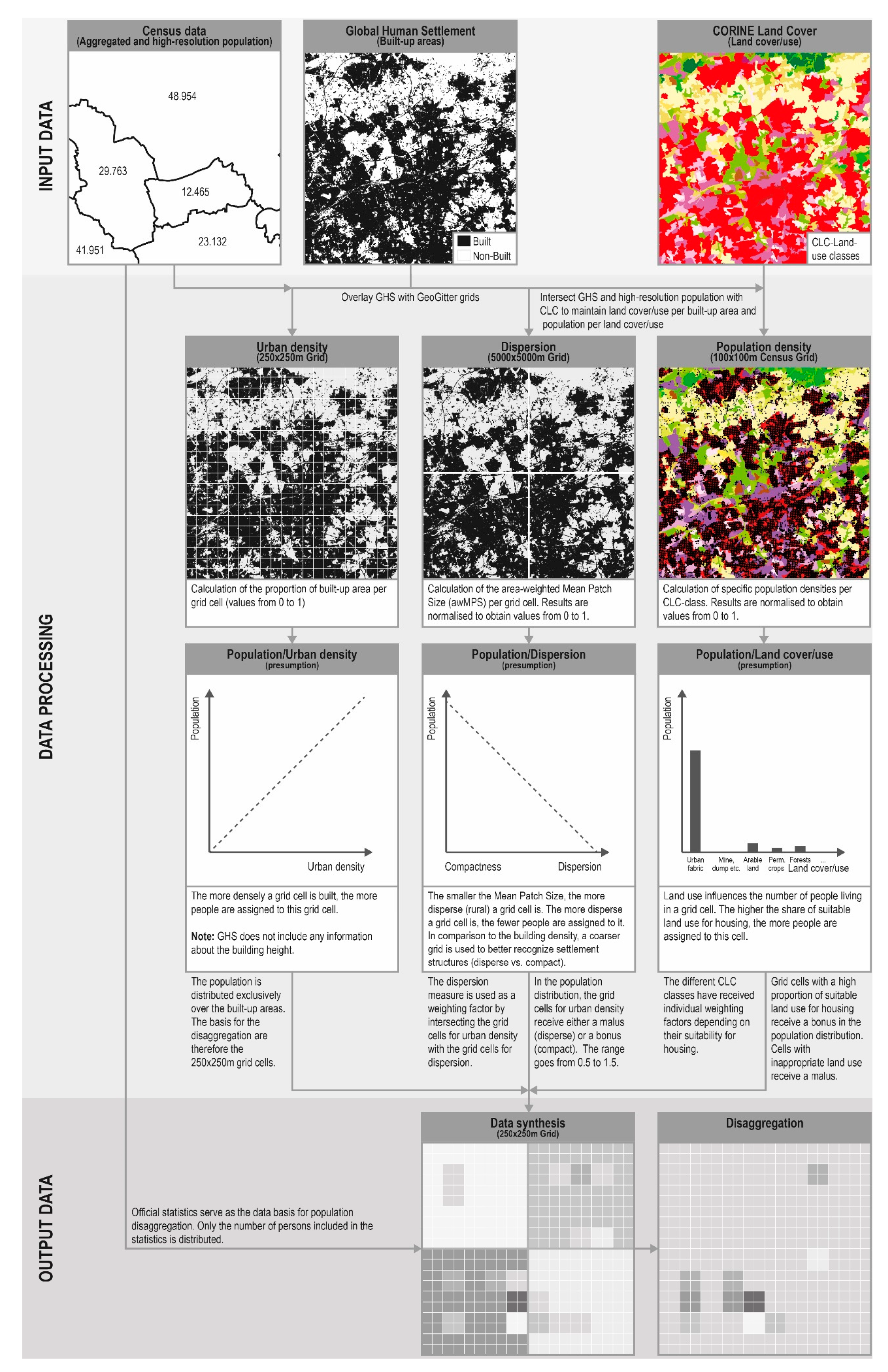
This article presents a dasymetric-based approach for modeling high-resolution population data in Germany based on four population distribution algorithms that disaggregate the population using census data, data of CORINE Land Cover (CLC) as well as the Global Human Settlement (GHS). Specifically, the population is spatially distributed through urban density, a spatial dispersion measure and the type of land cover/use. On the one hand, the novelty of this approach lies in the application of a spatial dispersion measure (area-weighted Mean Patch Size) to estimate population, and on the other hand, in the interaction of the different algorithms on the overall distribution accuracy. Besides, the article aims to contribute to the scientific debate by putting a special emphasis on the evaluation of results. While the majority of studies use standard methods like the mean absolute error (MAE) or root mean square error (RMSE) for the evaluation [5,21,36,40,41], the additional test procedures Gini-coefficient and local Moran’s I are applied to analyze the spatial effects of the algorithms.

The article is organized as follows: After this short introduction and literature review, Section 2 presents the materials and methods used to develop and evaluate the disaggregation algorithms. Section 3 shows the central results of the disaggregation algorithms structured by the accuracy assessment of the applied test statistics. The article concludes with a discussion of the benefits and limitations of the algorithms and accuracy assessments and gives an outlook for further research needs.

2. Materials and Methods

Built-up areas are inherent components of human settlements. They form the shape and appearance of a city and, in addition to technical and social infrastructures, also include the houses and apartments in which people live. Built-up areas can, therefore, be regarded as a suitable proxy for the distribution of the population. Since 2015, the GHS dataset is a new, high-resolution dataset on built-up areas. This dataset contains a global set of multi-temporal and multi-resolution grids. With a resolution of up to 30 m, this dataset differentiates between built-up and non-built-up areas for the years 1975, 1990, 2000 and 2014 [42]. The dataset offers the possibility to derive a multi-temporal and high-resolution population distribution worldwide and is used as a proxy for buildings in the present study. To ensure consistency with the other data used, the GHS data from 2014 was applied for population distribution.

The number of the population is highly correlated with land cover/use types [26,27]. The basic assumption is that certain types of land cover/use are associated with a more intensive residential use than others. It can be expected, for example, that a built-up area overlaid by a urbanized land cover is more likely to be characterized by a higher building density and a higher proportion of multi-family houses than a built-up area overlaid by agricultural land, where a higher proportion of one- and two-family houses or farmhouses is more likely. Therefore, datasets on land cover/use provide useful additional information to accurately distribute the population. In this study, the CLC dataset is used for this purpose. Since CLC is a harmonized and European-wide dataset, previous studies have already used it to develop and test algorithms for population distribution in Europe [27]. The dataset has a scale of 1:100,000, a geometric accuracy better than 100 m and contains 44 classes for land use within a 3-level hierarchical classification system. The survey dates are 1990, 2000, 2012 and 2018. In this study, data from 2012 were used to achieve the best possible temporal harmonization with the GHS dataset.

The data basis for the population are the annually updated population figures by the Federal Statistical Office within the framework of the ongoing spatial monitoring of the Federal Institute for Research on Building, Urban Affairs and Spatial Development (BBSR). The population figures are updated based on the results of the census of 9 May 2011. As already mentioned, and to achieve a temporal harmonization, population data from 2014 were used. In addition to the aggregated population data at the level of counties, cities and municipalities, high-resolution population data of the census grid from 2011 was also used.

In the following sections, the developed algorithms for population distribution are presented. Two assumptions build the basis for the developed algorithms: First, the population is redistributed exclusively to the built-up areas included in the GHS dataset. Second, the official population size determines the maximum number of people available for redistribution (pycnophylactic) to smaller spatial units [43].

The first algorithm distributes the population according to urban density. For this purpose, the built-up areas from the GHS dataset were transferred to another reference system. The GeoGitter of the Federal Agency for Cartography and Geodesy was used here, which is a two-dimensional multi-resolution geographic grid that meets the requirements of both INSPIRE Grids and national grid systems [44]. Since urban densities are mainly visible on a small scale, a grid with cell sizes of 250 × 250 m was applied. Based on pre-testing different cell sizes (100, 250, 500 and 1 km²), this grid provided the best compromise between accurate results and acceptable computing times. These outcomes are consistent with the results of [45]. With this grid, it is possible to determine the share of the built-up area within a bigger area (grid cells). Urban density thus indicates the share of built-up area in each grid cell and can, therefore, reach values between 0 (no built-up area) and 1 (fully built-up). Based on [45,46], a linear and constant relationship between urban and population density within a given region (e.g., county) is assumed. The distribution is based on a weighted sum function and is defined as

$$P={\displaystyle \sum }_i{A}_i\ast U{D}_i\ast k$$

(1)

$$k=\frac{P}{{{\displaystyle \sum }}_i{A}_i\ast U{D}_i}$$

(2)

where $P$ is the population in a given region, $U{D}_i$ is the urban density of grid cell $i$ and $A_i$ is the built-up area in grid cell $i$. $k$ describes the relationship between the urban and population density in a given region.

The second algorithm combines urban density with ancillary information on land cover/use. Therefore, the GHS dataset was enriched with information on land cover/use coming from the CLC dataset. Each CLC-class receives a specific weighting factor expressing the intensity of use for residential purposes. In contrast to other approaches, which just mask out specific CLC-classes for population distribution [47], this procedure has the advantage that all CLC-classes receive population depending on their specific weighting factor. Related approaches have already been tested and applied [27,48]. To map the intensity of residential use, the weighting factor was formed from specific population densities for all CLC-classes. For this purpose, the above-mentioned high-resolution population data from the 100 x 100 m census grid from 2011 were used. Here, the high-resolution population data were merged with the CLC-classes and the sum of population and the total area per CLC-class were calculated. To obtain population densities per CLC-class, the population was then divided by the total area of the respective CLC-class, as shown in Equation (3):

$$LU{D}_i=\frac{{\displaystyle \sum }LU{A}_i}{{\displaystyle \sum }{P}_i}$$

(3)

where $LU{D}_i$ is the population density of land cover/use class $i$, $LU{A}_i$ is the area of land cover/use $i$ and $P_i$ is the population located in land cover/use class $i$.

Since the GHS dataset does not contain any information on building heights, the integration of information on land cover/use and specific population densities using existing high-resolution census data allows an approximation to region-specific building structures. To do justice to region-specific population densities (e.g., sparsely populated rural counties or urban counties), population densities per CLC-class were determined separately for all given counties. As expressed in Equation (4), the calculated population densities were normalized with the min-max method (0 to 1) for a given region to include them as weighting factors. Equation (5) shows that the normalized density values are integrated as multipliers. Here, multipliers are applied to all land cover/use classes existing in each grid cell.

$$LU{D}_{i, norm}=\frac{\left(LU{D}_i-LU{D}_{min}\right)}{\left(LU{D}_{max}-LU{D}_{min}\right)}$$

(4)

$$P={\displaystyle \sum }{A}_i\ast U{D}_i\ast LU{D}_{i,norm}\ast k$$

(5)

The third algorithm combines urban density with additional information on dispersion respectively the compactness of settlement structures. The algorithm is based on the assumption that compact settlement structures are urban and disperse settlement structures are rural. According to this definition, it is more likely to have more people in compact settlement structures than in disperse. This assumption is based on the fact that urban regions are more characterized by multi-family houses than rural regions, which means that a larger number of people can be located there. To map compact or disperse settlement structures, the area-weighted Mean Patch Size (awMPS) was used. awMPS equals the sum, across all patches in a given landscape, of the corresponding patch metric value multiplied by the proportional abundance of the patch, i.e., patch area divided by the sum of patch areas. The awMPS is defined as

$$awMP{S}_i={\displaystyle \sum }(P{A}_i\ast \left(\frac{P{A}_i}{{\displaystyle \sum }P{A}_i}\right))$$

(6)

where $awMP{S}_i$ is the area-weighted mean patch size of grid cell $i$ and $P{A}_{ij}$ is the area of patch $j$ in grid cell $i$.

In comparison to the calculation of urban density, a coarser grid was used here to better recognize supra-local settlement structures. As with urban density, a grid from the GeoGitter framework was applied. In this study, a grid with a cell size of 5 × 5 km was used. Depending on the calculated $awMP{S}_i$, grid cells receive either a malus (low values = disperse) or a bonus (high values = compact). For this purpose, $awMP{S}_i$ was normalized with the min-max method and then added with 0.5, so that values between 0.5 and 1.5 could be achieved, as shown in Equation (7). Analogous to the second algorithm, the normalized dispersion measure is integrated as a multiplier in Equation (8).

$$awMP{S}_{i,norm}=\left(\frac{\left(awMP{S}_i-awMP{S}_{min}\right)}{\left(awMP{S}_{max}-awMP{S}_{min}\right)}\right)+0.5$$

(7)

$$P={\displaystyle \sum }{A}_i\ast U{D}_i\ast awMP{S}_{i,norm}\ast k$$

(8)

The fourth algorithm combines all three components and distributes the population based on urban density, land cover/use and the dispersion measure. Therefore, the distribution of population per grid cell was performed using the built-up area per grid cell as the basis $A_i$ weighted by urban density $U{D}_i$, population density per CLC-class $LU{D}_{i,norm}$ and the dispersion measure $awMP{S}_{i,norm}$. The fourth algorithm is defined as

$$P={\displaystyle \sum }{A}_i\ast U{D}_i\ast LU{D}_{norm}\ast awMP{S}_{i,norm}\ast k$$

(9)

Figure 1 gives a graphical overview of the entire procedure of the distribution algorithms and the databases used.

An important step in the development of distribution algorithms is the evaluation of the accuracy of the estimation. In the scientific literature, there exists a large number of different test statistics, which are also used as a basis for this study. The starting point for the accuracy assessment is the distribution of the population at the county level. Here, the population is first distributed to the grid cells (250 × 250 m) as shown in Figure 1, before the population is aggregated at the level of the municipalities. The results are then validated by comparing the modeled population with the official population of the municipalities. In total, six test statistics were used to test the algorithms on distribution accuracy, on the one hand, in terms of numbers and, on the other hand, in terms of systematic spatial deviations.

Mean absolute error (MAE) measures the average magnitude of errors in a set of predictions, without considering their direction [49]. With the help of MAE, the accuracy of the distribution can be represented numerically. Here, the quality of the algorithms increases when MAE becomes smaller. This means that with a small MAE, the modeled population deviates less from the actual population distribution. MAE is defined as

$$MAE=\frac{{{\displaystyle \sum }}_{i=1}^n\left(y_i-x_i\right)}{n}$$

(10)

where $y_i$ is the prediction and $x_i$ the true value.

Mean absolute percent error (MAPE) represents the percentage deviation between the predicted and the actual population of a reference unit. MAPE is defined as:

$$MAPE=\frac{1}{n}{\displaystyle \sum }\frac{\left(y_i-x_i\right)}{x_i}\ast 100$$

(11)

where $y_i$ is the prediction and $x_i$ the true value.

MAPE is used in this study because, unlike MAE, it allows a direct comparison between different reference units, as it removes the bias in the deviations caused by different population sizes.

Root mean square error (RMSE) is the standard deviation of the residuals (prediction errors). The effect of each error on RMSE is proportional to the size of the squared error, so, in comparison to MAE, the RMSE gives greater weight to larger errors than smaller ones, which shifts the error estimate towards outliers [49]. As a result, RSME is either equally high or higher than MAE. RSME is defined as

$$RMSE=\sqrt{\frac{{{\displaystyle \sum }}_{i=1}^n{\left(y_i-x_i\right)}^2}{n}}$$

(12)

where $y_i$ are the expected values, $x_i$ the observed values, and $n$ the total number of values.

In this study, RSME is applied as a test statistic especially because it highlights large errors. RSME can thus be used to check whether the average error has its origin in individual high error values, indicating that single municipalities are particularly over- or underestimated.

In addition, MAE, MAPE and RSME are applied to different types of municipalities and counties to test whether certain settlement structures are systematically over- or underestimated. Here, classifications developed by the BBSR are used. From the author’s point of view, they are suitable for this analysis since the delimitation criteria are population size, population density and population distribution.

Table 1. Types of municipalities and counties by the BBSR.

Region Type	Definition
Type of Municipality
Large city	at least 100,000 inhabitants
Large town	20,000 to less than 100,000 inhabitants
Medium town	10,000 to less than 20,000 inhabitants
Small town	5000 to less than 10,000 inhabitants
Rural municipality	under 5000 inhabitants
Type of County 1
Large city	at least 100,000 inhabitants
Urban county	(1) min. 50% and (2) min. 150 or (3) min. 150
Rural county with compaction tendencies	(1) min. 50% and (2) under 150 or (3) min. 100
Sparsely populated rural county	(1) under 50% and (3) under 100

¹ The types of counties are defined on the basis of three criteria: (1) population share in large and medium towns and (2) population density (inhabitants per km²) or (3) population density excluding large and medium towns.

lists the types of municipalities and counties and their specific delimitation criteria.

The coefficient of determination R² is a key figure for assessing the goodness-of-fit of a regression. The higher the coefficient of determination, the better the estimated values can represent the actual values. R² is defined as

$$R^2=\frac{n({\displaystyle \sum }xy)-({\displaystyle \sum }x)({\displaystyle \sum }y)}{\sqrt{\left[n{\displaystyle \sum }{x}^2-{({\displaystyle \sum }x)}^2\right]}\left[n{\displaystyle \sum }{y}^2-{({\displaystyle \sum }y)}^2\right]}$$

(13)

where $R^2$ is the correlation coefficient, $x$ are the values of the first dataset, $y$ are the values of the second dataset and $n$ is the total number of values.

The measure is used in the present study to compare the goodness-of-fit of the developed algorithms globally. However, MAE, MAPE, RSME and R² show weaknesses in testing for systematic spatial deviations. Therefore, the test statistics Gini-coefficient and local Moran’s I were performed.

The Gini-coefficient is a useful instrument for identifying and revealing concentration patterns [50]. The Gini-coefficient is derived directly from the Lorenz-curve and takes a value between 0 (with an even distribution) and 1 (if only one municipality receives the entire population, i.e., with a maximum unequal distribution). The Gini-coefficient is defined as

$$G=\frac{{{\displaystyle \sum }}_{i=1}^n{{\displaystyle \sum }}_{j=1}^n\left(x_i-x_j\right)}{2n^2\overline{x}}$$

(14)

where $x$ is an observed value, $n$ is the number of values observed and $\overline{x}$ is the mean value of $x$.

With its help, the behavior of the algorithms was tested for the concentration or even distribution of the population. For this purpose, the Gini-coefficient was calculated for the county types introduced in Table 1: firstly, for the actual population distribution and secondly, for the modeled population distributions. The coefficients indicate how the population is distributed among the municipalities within each county type. A comparison of the coefficients enables to analyze whether the modeled population is distributed more strongly to single municipalities or not.

Local Moran’s I is a test for spatial autocorrelation, which examines whether a phenomenon is clustered at a local level using local spatial autocorrelation [51]. It indicates if spatial autocorrelation is positive or negative and provides a p-value for the level of autocorrelation. Local Moran’s I is defined as

$$I_i=\frac{x_{i-\overline{X}}}{S_i^2} {\displaystyle \sum }_{j=1,j\ne i}^n{w}_{ij}\left(x_j-\overline{X}\right)$$

(15)

where $x_i$ is an attribute for feature $i$, $\overline{X}$ is the mean of the corresponding attribute, $w_{ij}$ is the spatial weight between feature $i$ and $j$.

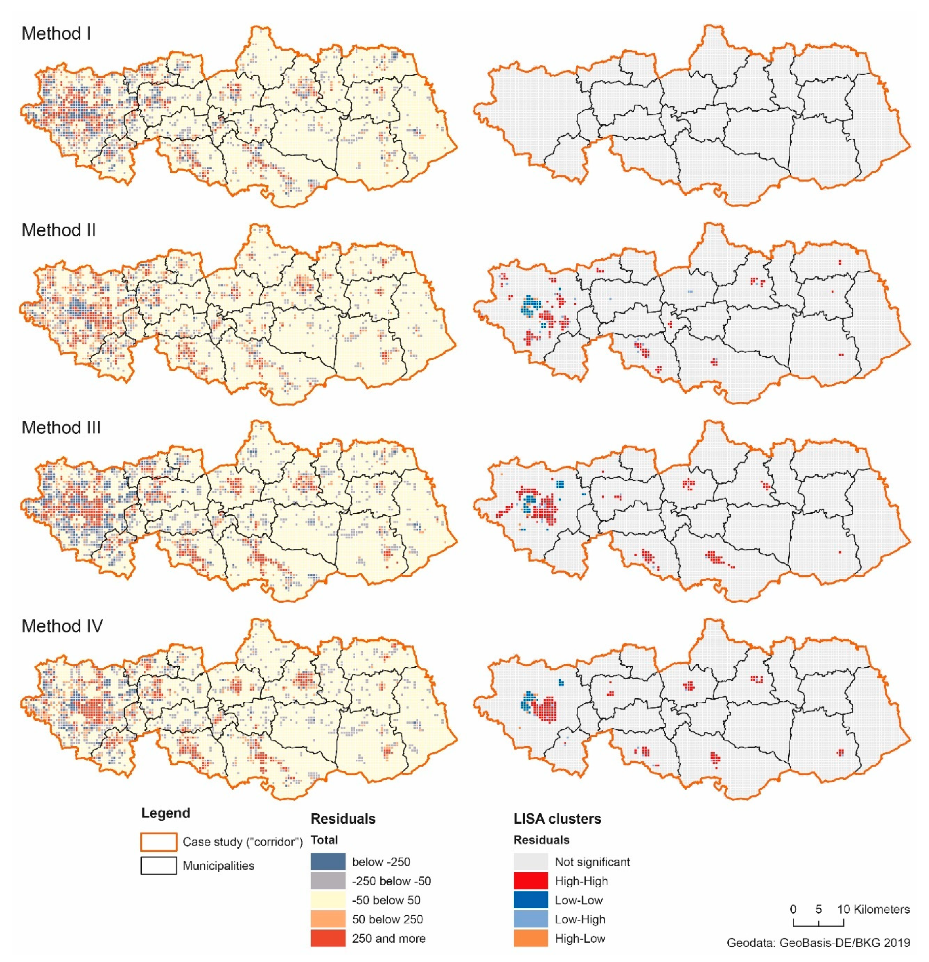
In this study, local Moran’s I was used twofold. On the one hand, it was used to check whether the developed distribution algorithms form spatial clusters with significant, high or low, positive or negative deviations on the level of municipalities, visible by the Local Indicators of Spatial Association (LISA clusters). Islands without any neighbor were excluded from the analysis. To obtain the most accurate results possible, a number of 99.999 permutations were applied. The calculations were performed with the software Geoda. The software has the advantage that no previous programming knowledge is required. Besides, the software is intuitive to use. To identify spatial clusters, the positive and negative absolute errors calculated for each municipality were used and the Benjamini–Hochberg procedure respectively False Discovery Rate (FDR) was applied [52]. FDR is a quality criterion that measures the correctness of all accepted hypotheses and, as a target value, allows a trade-off between as few “false discoveries” as possible, but still as many correct hits as possible. This ensures that the significance level is chosen in such a way that the FDR does not become too high.

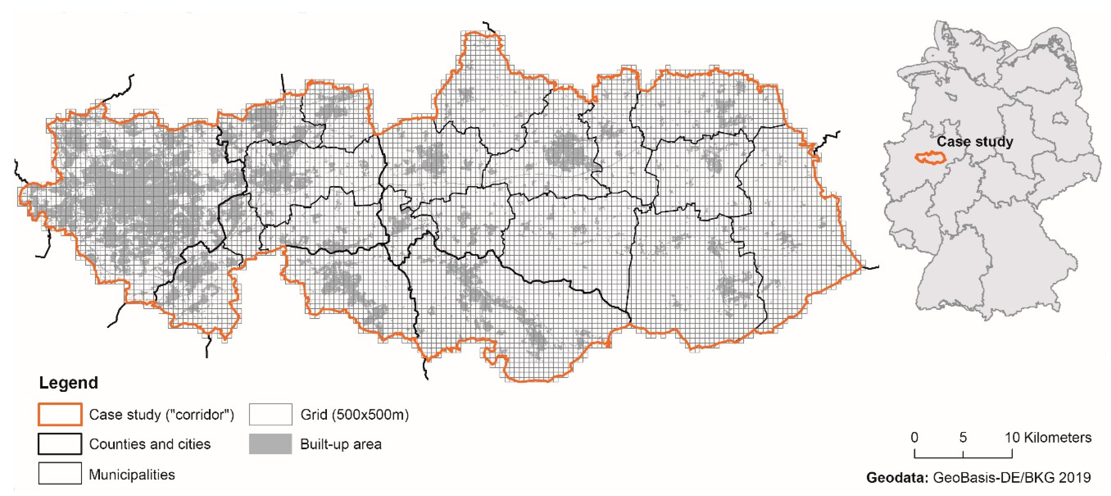
On the other hand, local Moran’s I was performed to analyze whether the distribution algorithms can estimate population distribution on a sub-municipality level correctly. For this purpose, a region (“corridor”) was selected that extends from the city of Dortmund, North Rhine-Westphalia, approximately 90 km to the east (Figure 2). This sub-region includes 20 municipalities and covers dense urban areas and peripheral rural areas. Therefore, the sub-region is suitable for analyzing the behavior of the algorithms on a sub-municipality level for different territorial categories. Methodically, the modeled population was compared with the population from the census grid 2011. To achieve this, for each cell of the corridor, the absolute deviation between the modeled and actual population was calculated. Since the census population is available in a 100 × 100 m grid and the modeled population was only disaggregated to a 250 × 250 m grid, both datasets were aggregated to a 500 × 500 m grid for better comparability. In addition, the deviations of the population within the corridor was investigated using concentric rings. The aim was to analyze the accuracy of the algorithms concerning the urban-rural gradient, which is mapped via the corridor. Starting from the most western point of the corridor, rings with a width of 10 km were generated. Within these rings, deviations between the census population and the modeled population were summed up and compared.

3. Results

In the following sections, the evaluation results for the algorithms developed are presented. The evaluation results are ordered according to the test statistics applied. Figure 3 shows the results of the four algorithms in a cartographic form.

3.1. MAE, MAPE and RSME

A look at the results across all municipalities shows that the distribution algorithms can map the actual population. Nevertheless, there are significant differences in the accuracy of the results. The sole application of urban density comes down to a MAE of 1.710 and a MAPE of 14.1%. The integration of the dispersion measure does not lead to improvements (MAE: 2.965, MAPE: 23.6%). The overall deviation of the distribution even increases. In contrast, the integration of land cover/use leads to a higher matching between the modeled and actual population. Here, a MAE of 1.483 was realized, which corresponds to a MAPE of 12.4%. A differentiated analysis of the results according to the different types of municipalities and counties (Table 1) shows a similar picture. The above-mentioned tendencies can also be observed across all types of municipalities and counties (

Table 2. MAE, MAPE (%) und RSME by types of municipalities.

		Rural Municipalities	Small Towns	Medium Towns	Large Towns	Large Cities
Population	Total	8,497,501	11,100,695	12,773,017	23,273,476	25,567,262
Method I	MAE	1.380	1.930	2.634	4.284	2.603
	%	27.1	21.4	18.1	11.5	0.8
	RSME	2.044	2.785	3.657	6.021	10.177
	%	40.1	30.8	25.1	16.1	3.1
Method II	MAE	1.281	1.653	2.179	3.748	3.038
	%	25.2	18.3	15.0	10.0	0.9
	RSME	1.772	2.209	2.887	5.439	14.514
	%	34.8	24.5	19.8	14.6	4.5
Method III	MAE	1.907	2.819	4.269	9.344	4.887
	%	37.4	31.2	29.3	25.1	1.5
	RSME	2.690	3.835	5.758	13.399	13.361
	%	52.8	42.5	39.6	35.9	4.1
Method IV	MAE	1.862	2.512	3.840	8.754	4.394
	%	36.6	27.8	26.4	23.5	1.4
	RSME	2.459	3.282	5.313	12.716	12.461
	%	48.3	36.3	36.5	34.1	3.9

and

Table 3. MAE, MAPE (%) und RSME by types of counties.

		Sparsely Populated Rural Counties	Rural Counties with Compaction Tendencies	Urban Counties	County-Free Cities
Population	Total	12,220,936	14,035,271	31,387,394	23,568,350
Method I	MAE	1.916	2.007	2.518	47
	%	22.3%	19.0%	14.3%	0.0%
	RSME	3.110	3.029	4.312	85
	%	36.2%	28.7%	24.4%	0.0%
Method II	MAE	1.799	1.761	2.114	32
	%	21.0%	16.7%	12.0%	0.0%
	RSME	2.801	2.558	4.358	66
	%	32.6%	24.2%	24.7%	0.0%
Method III	MAE	3.107	3.236	4.439	50
	%	36.2%	30.6%	25.2%	0.0%
	RSME	5.454	5.562	7.569	105
	%	63.5%	52.7%	42.9%	0.0%
Method IV	MAE	3.085	3.160	3.814	36
	%	35.9%	29.9%	21.6%	0.0%
	RSME	5.406	5.493	6.688	87
	%	63.0%	52.0%	37.9%	0.0%

).

A look at the RSME shows that the lowest values per municipality type are achieved with method II. The highest relative RSME values occur in the type of rural municipalities. Rural municipalities are thus more strongly characterized by outliers with high deviations. The difference between the relative deviations of MAE and RSME decreases when going from rural to urbanized municipalities (left to right), which means that outliers with high deviations occur here less frequently. The RSME increases particularly strongly when method III is used, which suggests a disproportionate increase in large outliers. The analysis for the county types shows a similar picture. The deviations are large in rural regions and smaller in urban areas. Methods III and IV perform worse and particularly poorly in sparsely populated areas. This is also illustrated by the large differences between MAE and RSME, which indicates a significant increase in outliers with high deviations. In short, rural territorial units show the highest deviations in the population distribution. Urban regions are better estimated in comparison. While MAE is lower for small and rural units, the percentage mean deviation from the mean population increases. RSME also shows that the error is higher in rural areas and is more marked by larger errors. This is particularly visible in sparsely populated counties using method III.

3.2. Coefficients of Determination R²

Figure 4 graphically compares the modeled population against the actual population. Here, a match of 100% would be visible as a straight diagonal line. This is not the case with any of the four algorithms developed. Nevertheless, a high degree of correlation is achieved. This correlation can be expressed by the coefficients of determination R². With method I an R² of 0.9516 is achieved. Method II achieves a value of 0.9555, method III achieves an R² of 0.9131 and method IV achieves a R² of 0.9195. These results are consistent with the results of MAE, MAPE and RSME, where method II performs best.

3.3. Gini-Coefficients

Overall and in comparison to the actual population, almost identical concentration patterns are achieved across all algorithms and all county types (Figure 5). The algorithms result in marginally lower concentration patterns in the categories (a) cities and (b) urban counties compared to the actual population distribution, visible by the dashed line, which is located further away from the diagonal line. In contrast, the population distribution in the municipalities of the (d) sparsely populated rural counties shows slightly higher concentration patterns, which means that the algorithms assign higher population numbers to single municipalities. Nevertheless, the observable differences are very small.

The optical evaluation of the Lorenz-curves is reflected in and confirmed with the Gini-coefficients in

Table 4. Gini-coefficients by distribution algorithm and type of county.

	Actual Distribution	Method I	Method II	Method III	Method IV
Types of counties
Sparsely populated rural counties	0.304	0.359 (0.055)	0.362 (0.058)	0.363 (0.059)	0.368 (0.064)
Rural counties with compaction tendencies	0.362	0.339 (−0.023)	0.334 (−0.028)	0.338 (−0.024)	0.342 (−0.020)
Urban counties	0.362	0.329 (−0.033)	0.335 (−0.027)	0.329 (−0.033)	0.333 (−0.029)
Large cities	0.363	0.342 (−0.021)	0.344 (−0.019)	0.339 (−0.024)	0.340 (−0.023)
Municipalities	0.349	0.342 (−0.007)	0.343 (−0.006)	0.343 (−0.006)	0.347 (−0.002)

note: In the parentheses, the difference between the Gini-coefficient of the modeled and actual population distribution is given.

. For example, in sparsely populated rural counties, a slightly higher inequality of distribution is calculated, expressed by the positive number in the parentheses. In contrast, in large cities, urban counties and rural counties with compaction tendencies, the Gini-coefficient is lower than for the actual population distribution. This indicates that, due to the algorithms, populous municipalities receive less population which leads to a more equal distribution. However, the coefficients also show that the overall differences are very small. With differences between +0.064 and −0.033, it can be assumed that the concentration patterns of the actual population distribution are largely comparable and similar ratios between the share of municipalities and the share of the population are achieved.

3.4. Local Moran’s I

The local Moran’s I was calculated for the deviations of all four distribution algorithms. On the level of the municipalities, all four algorithms lead to the same result. No region in Germany is systematically under- or overestimated. Consequently, there are no significant spatial clusters of adjacent municipalities, with positive or negative values above average. To examine the spatial effects at the level below the municipality, a sub-region was analyzed (Section 2).

Figure 6 shows the MAE as well as the LISA clusters for all four algorithms in the case study region. Looking at Figure 6 (left), it is striking that, with all methods, the population in the center of the city of Dortmund in the western part of the case study region is mostly underestimated. The high negative deviations indicate that the algorithms are not able to estimate the population in this inner-city, high-density area sufficiently high, even with the calculated population densities per CLC-class used in method II. In comparison, the city districts around the city center tend to be overestimated. An exception is method III, where these spatial patterns are partially reversed. The underestimation of the urban core area is less pronounced. In contrast, the suburbs show underestimations.

In the eastern municipalities of the case study region, the methods produce similar spatial outliers in terms of the modeled population distribution. The trend that could be observed in the more urbanized areas is reversed in the less urbanized municipalities. Here, high positive deviations can be found in the urban core areas in particular. In contrast, negative deviations can be seen in city districts further away from the city centers. Overall, it is noticeable that the absolute deviations are significantly lower than in the western part of the case study region, and the distribution of the deviations is more disperse. However, the lower occurrence of absolute deviations is also due to the lower absolute population number in these municipalities’ respective grid cells.

The maps of the LISA clusters reflect what the analysis of the residuals has already indicated (Figure 6: right). For method II, III and IV, there are spatial clusters of high overestimations in Dortmund in the city districts away from the city center and a spatial cluster of high underestimations in the city center. Using methods II and III, the distribution of spatial clusters is more disperse. In comparison, method IV produces just three spatial clusters with a clear concentration on the urban core area. In rural areas, there are high–high clusters mainly in the urban core areas. As Figure 6 shows, the spatial distribution of the LISA clusters is very similar for methods II–IV. The clusters differ only in their spatial characteristics and extent. It is noteworthy that method I has no spatial clusters, which means that no deviations above the average could be found here.

A look at the population distribution by concentric rings shows that the algorithms can map the actual population distribution well (Figure 7). The general trend of the official population is visible and comparable. However, the residuals in Figure 7 show a differentiated picture regarding the different methods. The deviations in method I and II are at a moderate level, whereas the deviations in method II are even smaller. The deviations of method I are only smaller in the 20- and 40-km rings. In contrast, the positive and negative deviations of method III and IV are significantly higher. Method III and IV underestimate the 10-km ring and greatly overestimate the 20-km ring. The rings from 40 to 60 km are also overestimated, although the differences are not as strong as in the more urbanized rings. With the 70-km ring, there is again a stronger underestimation of the population.

4. Discussion

The accuracy assessments show a differentiated picture of the results achieved with the algorithms developed. Overall, the methods I and II perform better than the methods III and IV, where the deviations are mostly higher. In terms of accuracy, the results produced are comparable to the results of previous studies [26,27,45] that used similar databases.

Using urban density only, acceptable results can be achieved. However, urban density—as operationalized in this study—also results in highly dense areas being underestimated. The reason for this is that if a cell is fully built-up, the same number of people is allocated to it, irrespective of the cell being located in a city or a village. This bias can also not be resolved with higher-resolution data like GHS, as it still does not include any 3D information. A combination of 2D data with region-specific density values as applied in this study can only be understood as a proxy to consider this vertical dimension of a city. Therefore, data on building heights and volumes will play a crucial role in estimating population in the future. To date, the number of studies using building data is small and limited to case studies [22,53,54,55]. On the one hand, this may be due to the fact that the data is not always be publicly available and, on the other hand, data processing is more complex and requires more computing power.

The accuracy assessment confirms that data on land cover/use is an important ancillary source of information to enable a correct and accurate population distribution. Both at the municipal and sub-municipal level, the usage of land cover/use data improves the accuracy of the results. But the determination of specific densities per CLC-class is not sufficiently high to correctly estimate the very dense inner-city areas as shown for the sub-municipal level. This may be because the region-specific densities are determined on the level of counties and thus primarily represent only average values for a region. If there are few dense and many rural municipalities in a county, this may cause the region-specific density values to underestimate the density values of dense municipalities.

The dispersion measure, in general, does not improve the overall distribution accuracy. While the dispersion measure leads to improvements in a few municipalities, the quality of distribution is worse overall. The results suggest that disperse or compact settlement structures—in the sense of the measuring method used here—have a low or subordinate significance for the distribution of the population. One reason for this may be that even in disperse settlement structures, high building densities may occur on a small scale. These small-scale outliers are not detected by the method. On the other hand, this may be due to the data basis used. For instance, a single pixel can cause several smaller patches to be treated as one large patch, even though the built-up areas are not connected. This phenomenon is particularly likely to occur in urban areas, where many patches lay close to each other. In terms of population distribution, urban areas can, therefore, be estimated less accurately for two reasons. On the one hand, compact structures receive per se a bonus in the sense of the developed methodology, and on the other hand, the measurement method and the data basis lead to cities erroneously forming large patches. Hence, it cannot be ruled out that the measurement of settlement structures as a whole may lead to less plausible results.

Overall, smaller and more rural regions have poorer estimation results. This result applies both to the municipalities and to the types of municipalities and counties. One reason for this is the quality of the data basis used. Especially the minimum cartographic unit (MCU) of 25 ha of CLC can lead to higher errors in rural areas since it results in land cover/use classes below this threshold being integrated into surrounding classes above this threshold. Thus, not all small settlements in rural areas are recognized and displayed with CLC. For instance, small urbanized patches in rural areas are likely to be integrated into the surrounding agricultural land. As a result, lower population densities are assumed and assigned for built-up areas in these classes. As a consequence, these settlements receive a lower weight in the population distribution. This limitation is already recognized in previous studies [26,27]. The GHS data is a unique source of information, nevertheless, it also has limitations in terms of population distribution. First, the data is based on automatic remote-sensing built-up area recognition. This means that the detection of built-up areas is not error-free. Since the population is distributed exclusively over built-up areas, this can lead to biases. Second, the data differentiates exclusively between built-up and non-built-up areas. The data set, therefore, also includes large built-up areas which are not designated for residential purposes like transport infrastructures. This leads to population being distributed incorrectly here as well. Third, it was found that, despite the high resolution of the GHS, smaller and rural settlements are not always completely captured. In addition to the limitations imposed by the MCU of CLC, this can lead to further biases, especially in rural areas.

The results of the concentration measurements of the Gini-coefficient show that there are approximately identical concentration patterns in the distribution of the population, regardless of the method used. At the level of the municipalities, deviations in concentration patterns, therefore, seem to play a subordinate role. Nevertheless, the Lorenz-curves and the Gini-coefficients give—from the author’s perspective—a good overview of how the algorithms react to different settlement structures. In this study, the Gini-coefficient was calculated for municipalities, which limits the analytical power, but an application at every other spatial level (e.g., grid cells) is possible. Overall, the Gini-coefficient does not replace a detailed evaluation of results. With the help of the local Moran’s I, a more detailed analysis of the results is possible and it shows where the algorithms do not perform well. Especially when systematic errors appear, adjustments to coefficients or the ancillary data of the algorithms can be made for re-calibration. Iterations can then be used to check whether these errors could be corrected or not. The analysis below the level of the municipality is based on a comparison of the modeled population with the high-resolution census data. In the context of this study, deviations and inaccuracies in the evaluation may occur due to a time lag between the data used (2014 [modeled], 2011 [official]), that do not originate in the algorithms. For example, built-up areas may have been developed between 2011 and 2014 that are meanwhile populated, that are included in the GHS data but do not yet appear in the census data. A temporal harmonization of data is therefore particularly important to produce valid evaluation results.

Besides, rounding errors can occur in the population distribution as well as in the aggregation of the population from the grid cells to the municipal level. This becomes particularly clear in the case of large cities since here the population is distributed to only one administrative unit. But these errors play a subordinate role and are below 1% across all algorithms.

It should be noted that the availability of the data used here is currently no more frequent than in the census. However, the advantage of the distribution algorithms is that with different spatial data and national annual population aggregates an estimation for individual years can be made, which improves the availability of high-resolution data. In particular, the globally uniform GHS data allows an easy transfer and application of the developed algorithms to other areas of the world. However, the above-mentioned remarks show that the accuracy and quality of additional input data is of particular importance. Additional input data should, therefore, always be subject to preliminary checks to determine whether they are suitable for disaggregation or not.

5. Conclusions

The need for reliable, high-resolution population data will continue to grow in the years to come. Therefore, the further development of methods for high-resolution population disaggregation will remain an important field of research in the future. Besides, the development and establishment of appropriate and consistent evaluation methods is also a central part. As [56] have already pointed out, in recent years, work has mainly been done on the further development of powerful estimation methods. A discussion on the evaluation of results remained largely unaffected by this. As current studies show, test procedures have barely changed at all. A discussion on minimum standards for the evaluation of results would be useful from the authors’ point of view. On the one hand, to make estimation procedures more efficient and, on the other hand, to make them more comparable with each other. For future approaches to population distribution, the test statistics presented here can provide added value for testing accuracy.

Beyond that, the transferability of developed approaches to similar distributional issues seems desirable. For instance, high-resolution employment figures would be an important and profitable data basis for many research questions. From the author’s point of view, existing approaches show that the developments in the field of open data can be an important impetus for further progress. It can be assumed that new data sources will be developed and made available for similar and further research questions.