Tree Water Status in Apple Orchards Measured by Means of Land Surface Temperature and Vegetation Index (LST–NDVI) Trapezoidal Space Derived from Landsat 8 Satellite Images

Abstract

In this study, the split window (SW) method was applied for land surface temperature (LST) retrieval using Landsat 8 in two apple orchards (Glindow, Altlandsberg). Four images were acquired during high demand of irrigation water from July to August 2018. After pre-processing images, the normalized difference vegetation index (NDVI) and LST were calculated by red, NIR, and thermal bands. The results were validated by interpolated infrared thermometer (IRT) measurements using the inverse distance weighting (IDW) method. In the next step, the temperature vegetation index (TVDI) was calculated based on the trapezoidal NDVI/LST space to determine the water status of apple trees in the case studies. Results show good agreement between interpolated LST using IRT measurements and remotely sensed LST calculation using SW in all satellite overpasses, where the absolute mean error was between 0.08 to 4.00 K and root mean square error (RMSE) values ranged between 0.71 and 4.23 K. The TVDI spatial distribution indicated that the trees suffered from water stress on 7 and 23 July and 8 August 2018 in Glindow apple orchard with the mean value of 0.69, 0.57, and 0.73, whereas in the Altlandsberg orchard on 17 August, the irrigation system compensated the water deficit as indicated by the TVDI value of 0.34. Moreover, a negative correlation between TVDI and vegetation water content (VWC) with correlation coefficient (r) of −0.81 was observed. The corresponding r for LST and VWC was equal to −0.89, which shows the inverse relation between water status and temperature-based indices. The results indicate that the LST and/or TVDI calculation using the proposed methods can be effectively applied for monitoring tree water status and support irrigation management in orchards using Landsat 8 satellite images without requiring ground measurements.

1. Introduction

Tree water status and the determination of appropriate irrigation measure can be supported by digital plant data as suggested in the context of precision horticulture [1,2]. Established methods for estimating water stress such as gravimetrically or electrically measured soil and plant water contents are not only time consuming, but also produce discrete local data points, which may not be representative of an entire field or orchard. To maximize water use efficiency, new irrigation management strategies are needed [3,4,5,6]. Irrigation needs in the orchard are influenced by weather, climate variables, soil, and plant response, which can be measured with thermal imaging [3,7,8,9,10,11]. Furthermore, irrigation scheduling considering regulated deficit irrigation, is based on crop response to water stress at different growth stages [12,13,14,15]. Increased leaf temperature and decreased vegetation (leaf) water content (VWC) are signs of water stress monitored with thermal imaging [16] that can be implemented in the orchard by crane, tractor, and unmanned aerial vehicle (UAV). However, one of the key parameter in vegetation water balance studies is land surface temperature (LST). In the past, the LST was measured by infrared thermometers which was costly and time-consuming. Since the 1980s, the remote sensing (RS), particularly satellite imagery, methods have been used for LST calculations [17,18,19]. From the satellite position, “surface” means whatever is seen from the atmosphere on the surface of the earth, e.g., in an apple orchard, the tree canopy is considered as a surface, ergo the LST equals predominantly to the leaf surface temperature. An early effort for calculating LST using RS methods was made using the advanced very high resolution radiometer (AVHRR) on the NOAA 7 satellite, which acquires 1-km spatial resolution data, and applying the split window algorithm [20]. After analyzing the relevant sources of errors, the author showed that the split window method could be adopted with an accuracy of 3 °C. Among numerous applications of LST retrieval calculations, its application is still followed in estimating water status in the field [21]. In this regard, many studies have been carried out for developing and improving the LST retrieval methods [22,23,24,25,26] to estimate evapotranspiration. Moreover, the RS has been utilized for estimating vegetation indices (VI), such as the normalized difference vegetation index (NDVI) [27]. The scatter plot of these remotely sensed indices (NDVI and LST) resulted in a trapezoidal space, which has a physical concept i.e., the spatial relation (trapezoidal space) between LST and NDVI is applied to monitor the water status of crops and orchards using temperature vegetation dryness index (TVDI) [28,29]. However, the TVDI reflects a mixed signal of the soil moisture under trees and leaf water content of trees.

Due to the relatively high resolutions and the free availability of all data by the U.S. Geological Survey (USGS), the Landsat 8 launched on 11 February 2013, with 9 operational land imager (OLI) and 2 thermal infrared sensor (TIRS) bands providing the prerequisites for calculating NDVI and LST. Using the TIRS bands provided, the calculation of the LST can be performed using either two thermal bands, e.g., split window (SW) algorithm, or one band such as single channel (SC) algorithm [30]. All of the indicated algorithms are based on the radiative transfer theory (RTT) equation. The Landsat 8 data for LST retrieval calculation was approached in northwest of China [31]. The authors applied SW algorithm and validated results with moderate resolution imaging spectroradiometer (MODIS) LST products.

Although many further studies applying satellite imagery for water status estimation based on land surface temperature (LST) were carried out in field crops, the application in orchards is still in its infancy. The present study was aimed at proposing a method for TVDI estimation based on partly mixed pixels in orchard conditions by means of (i) selecting an interpolation method for gaining spatial distribution data of LST based on infrared thermometer (IRT) measurements and approaching the SW method using Landsat 8 images. Subsequently, (ii) validate the results with ground reference measurements, and (iii) estimating TVDI considering the VWC.

2. Materials and Methods

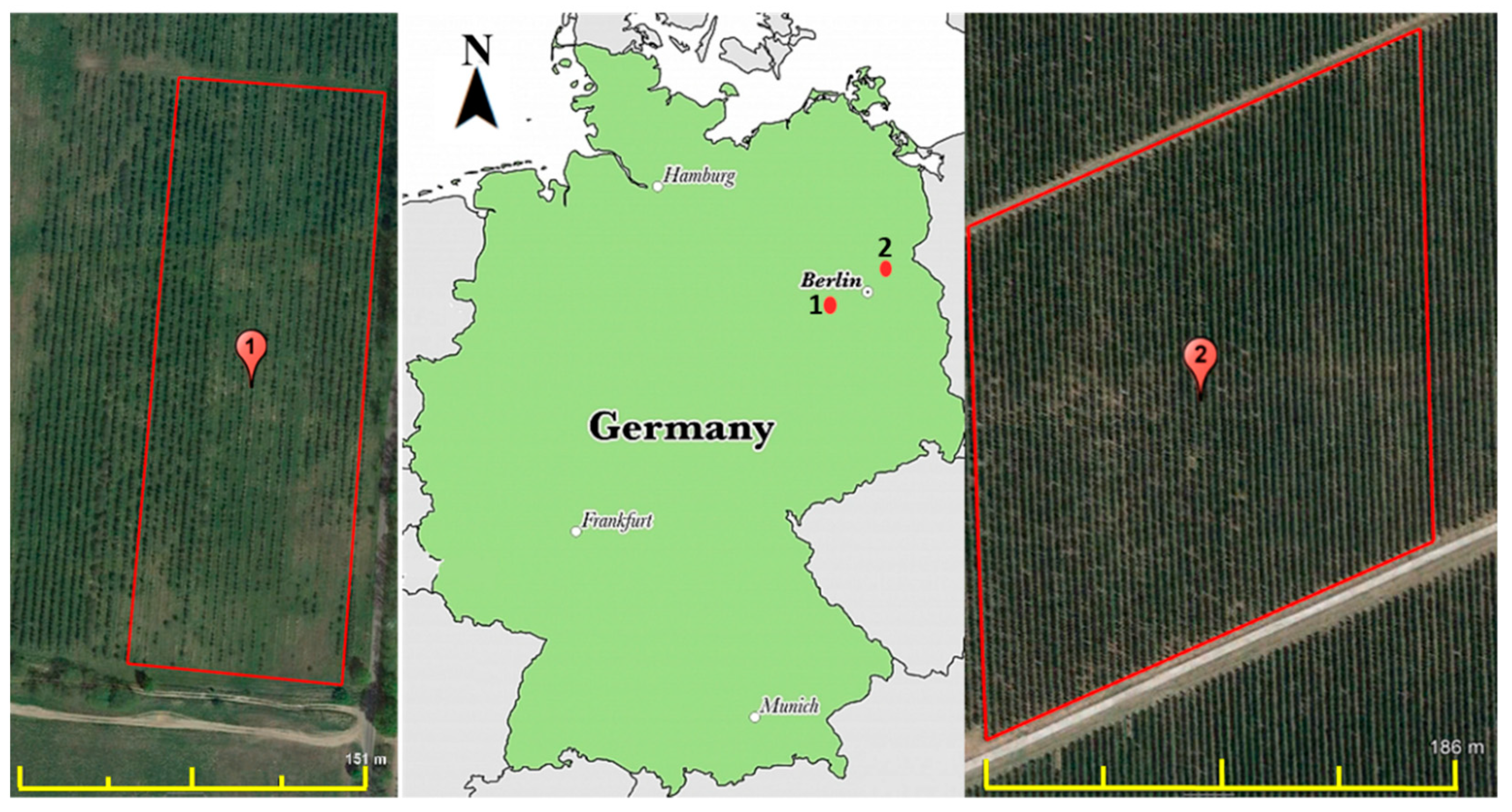
2.1. Study Area

In this study, two commercial apple orchards located in a fruit production area of Germany were selected: The Glindow’s commercial apple orchard with longitude and latitude of the field center being 52°21′15.8″ N 12°51′53.8″ E (path/row: 193/23 for Landsat 8 satellite images). The cultivar of the apple (Malus × domestica Borkh.) is ‘Pinova’, which was harvested 24 September 2018 in the present orchard. The Altlandberg’s commercial apple orchard located with longitude and latitude of the field center is 52°36′27.5″ N 13°49′3.07″ E (path/row: 192/23 for Landsat 8 satellite images) with the cultivar (Malus × domestica Borkh.) being ‘Gala’, was planted in 3.5 × 1.0 m distance. The common irrigation system in this area is drip irrigation. Both sites have semi-humid climate and are geographically surrounded by fruit orchards (Figure 1).

Daily meteorological data were recorded with weather stations (IMT280, Pessl, Austria) including air temperature, soil temperature in 5 depth, and relative humidity (RH).

2.2. Field Measurements

The LST and VWC were measured in 10 points during the Landsat 8 satellite overpasses on 7 and 23 July and 8 August 2018 between 11:00 to 12:00 in Glindow and 17 August 2018 in Altlandsberg. At each point, 20 representative leaves were sampled (n = 200) and canopy temperature was measured 20 times for each canopy using digital IRT (OS91, Omega, Norwalk, CT, USA) from sun and shade position of trees. The mean of these 20 values is considered as a representative of leaf temperature at each point.

The leaf samples were sealed in individual plastic bags, placed in a cool and dark container to avoid water losses on the return to the laboratory. Fresh weight (FW) of gathered samples was recorded immediately, and subsequently samples were oven-dried at 105 °C for 24 h until constant dry weight (DW) was reached. Finally, the VWC value was calculated for each sample (Equation (1)):

$$WC=(FW-DW/FW)\times 100\%.$$

(1)

2.3. Landsat 8 Satellite Image Acquisition and Data Preprocessing

Landsat 8 has 9 operational land imager (OLI) spectral bands in the range 0.45 μm (blue/visible) to 2.29 μm (infrared/nonvisible) and 2 thermal infrared sensor (TIRS) bands in the high infrared range (10.0–12.5 μm). Due to the relatively high horizontal resolution of the OLI bands (30 m), the frequent sweep of the satellite over the same corridor at the earth’s surface appeared in intervals of 16 days, which were free availability by the USGS (http://earthexplorer.usgs.gov). Four Landsat images were acquired during the high water demand months (July and August) of apple trees (

Table 1. Landsat 8 overpass over the orchards.

Path	Row	Date	Time *	Region
193	23	07 July 2018	12:01′:39″	Glindow
193	23	23 July 2018	12:01′:46″	Glindow
193	23	08 August 2018	12:01′:55″	Glindow
192	23	17 August 2018	11:55′:49″	Altlandsberg

* local time (Central European Summer Time = GMT+2).

).

In order to preprocess the satellite images, the digital numbers (DN) of TIRS and OLI bands were converted to spectral radiance and top of atmosphere (TOA) planetary reflectance. To convert DNs to radiance the formula below was used [32]:

$$L_{\lambda }=M_L\ast Q_{cal}+A_L,$$

(2)

where $L_{\lambda }$ is spectral radiance (W/(m² sr µm)), $M_L$ is radiance multiplicative scaling factor, $Q_{cal}$ is DN value of each pixel, and $A_L$ is radiance additive scaling factor. TIRS data were converted from spectral radiance to brightness temperature [32]:

$$B{T}_i=\frac{K2}{\ln (\frac{K1}{L_{\lambda }}+1)},$$

(3)

where $B{T}_i$ is top of atmosphere (TOA) brightness temperature for TIRS band $i$ (= 10, 11) in Kelvin. The K coefficients are thermal conversion constants for Landsat 8 TIRS bands (

Table 2. Thermal conversion constants.

Parameter i	K1	K2
Band 10	774.8853	1321.0789
Band 11	480.8883	1201.1442

).

The NDVI is computed by TOA planetary spectral reflectance, with solar angle correction. The DNs are converted to TOA planetary reflectance by the below equation [32]:

$${\rho }_{\lambda }=\acute{{\rho }_{\lambda }}/\sin \theta =(M_p\ast Q_{cal}+A_p)/\sin \theta ,$$

(4)

where ${\rho }_{\lambda }$ and $\acute{{\rho }_{\lambda }}$ are TOA planetary spectral reflectance with and without solar angle correction (unitless), $M_p$ is reflectance multiplicative scaling factor, $A_p$ is reflectance additive scaling factor, and $\theta$ is solar elevation angle. $M_L,A_L,M_p,A_p$, and $\theta$ parameters in Equations (2) and (4) are extracted from the metadata file, which is downloaded with satellite images from the USGS EarthExplorer.

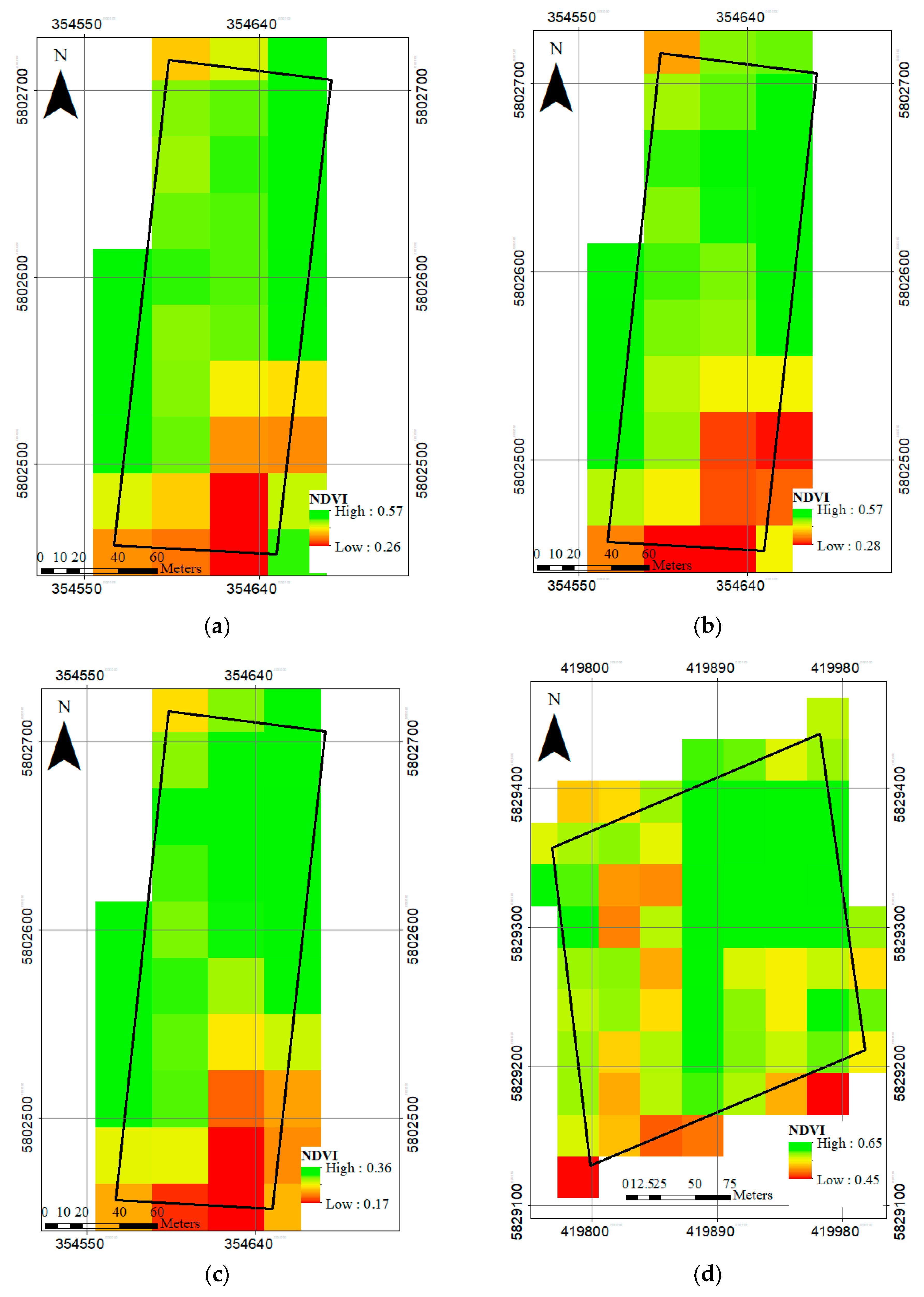
2.4. NDVI Calculation Using Landsat 8

After conversion of the DN to reflectance, the normalized difference vegetation index (NDVI) for the red and near infrared (NIR) bands was calculated by the following equation [33]:

$$NDVI={\rho }_{NIR}-{\rho }_{Red}/{\rho }_{NIR}+{\rho }_{Red}.$$

(5)

The value range of NDVI is −1 to 1, negative values of NDVI may point to water bodies and snow cover, while values greater than 0.5 indicate dense vegetation cover [34].

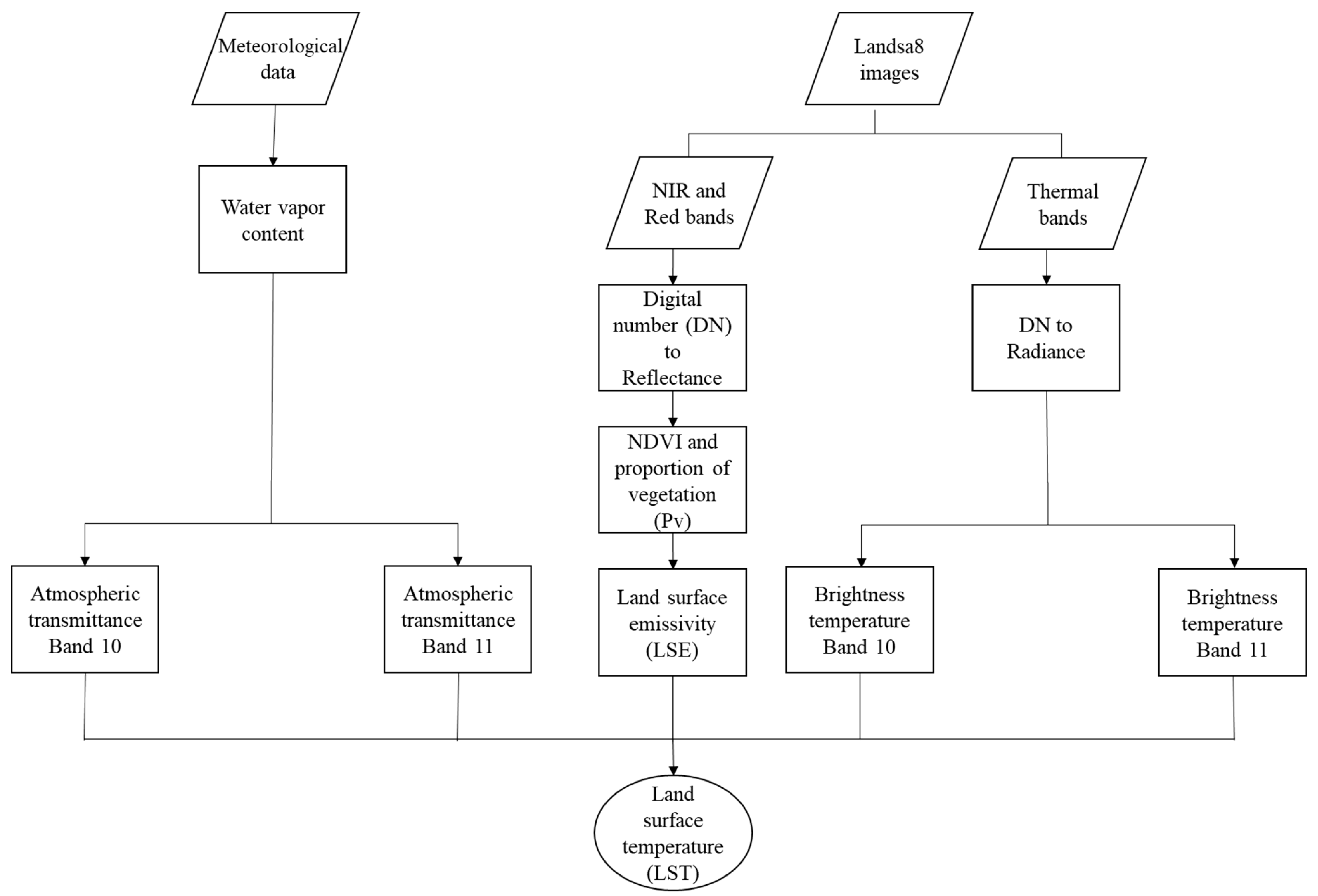
2.5. Radiative Transfer Theory (RTT) Equation and Split-Window (SW) Algorithm

A simplified radiative transfer equation expresses the apparent radiance received by a sensor [35,36]:

$$B_i(B{T}_i)={\tau }_i(\theta )\left[{\epsilon }_i{B}_i(LST)+(1-{\epsilon }_i)I_i^{\downarrow }\right]+I_i^{\uparrow },$$

(6)

where $B_i(B{T}_i)$ radiance received by channel i(=10, 11) of the sensor with brightness temperature $B{T}_i$; $B_i(T_s)$ is the ground radiance; ${\tau }_i(\theta )$ is atmospheric transmittance for channel i when viewing zenith angle is $\theta$. The Landsat-8 TIRS is at an altitude of 705 km with a swath of 185 km. Therefore, TIRS is treated as nadir viewing, since the maximum zenith viewing angle is not more than 7.5°, so the $\theta$ could be ignored i.e., on that angle, the effect on the atmospheric transmittance in TIRS band is negligible [37,38,39]. ${\epsilon }_i$ is land surface emissivity (LSE); $I_i^{\downarrow }$ and $I_i^{\uparrow }$ are down-welling and up-welling path radiance, respectively. Regarding the Plank’s law, $B_i(T)$ is calculated by:

$$B_i(T)=\frac{2h{c}^2}{{\lambda }_i^5\left(\exp \left(\frac{hc}{{\lambda }_{i}kT}\right)-1\right)}=\frac{C_1}{{\lambda }_i^5\left(\exp \left(\frac{C_2}{{\lambda }_{i}T}\right)-1\right)},$$

(7)

where c is light speed (2.9979 × 10⁸ m/s), h is Plank constant (6.6261 × 10⁻³⁴ J·s); k is the Boltzmann constant (1.3806 × 10⁻²³ J/K); and ${\lambda }_i$ is the effective center wavelength of band i which is equal to 10.9 and 12 μm for band 10 and 11 TIRS; $C_1$ is 1.19104 × 10⁸ Wμm⁴m⁻²sr⁻¹ and $C_2$ is 14387.7 μmK. By solving Equations (6) and (7), the LST could be estimated in Kelvin (K) for Landsat thermal bands (Equation (8)):

$$LST=\frac{C_1}{{\lambda }_{i}ln\left(\frac{C_2}{{\lambda }_i^5\left(B_i(B{T}_i)-I_i^{\uparrow }-{\tau }_i(1-{\epsilon }_i)I_i^{\downarrow }/{\epsilon }_i{\tau }_i\right)}+1\right)},i=10,11.$$

(8)

In order to retrieve LST from Landsat 8 TIRS bands by RTT equation, ${\tau }_i,I_i^{\downarrow }$, and $I_i^{\uparrow }$ could be analyzed by simultaneous measurements of radio sounding data during the time period of Landsat overpass. In automated applications, these types of data are not available, thus [40] simplified the RTT equation and proposed an algorithm for spilt window method by solving Equation (6) for the advanced very high resolution radiometer (AVHRR) data. Their proposed SW algorithm (Figure 2) was applied in the present study (Equation (9)):

$$LST=A_0+A_1\ast B{T}_{10}+A_2\ast B{T}_{11},$$

(9)

where A₀, A₁ and A₂ are calculated by:

$$A_0=\frac{\left[a_{10}{D}_{11}(1-C_{10}-D_{10})-a_{11}{D}_{10}(1-C_{11}-D_{11})\right]}{(D_{11}{C}_{10}-D_{10}{C}_{11})},$$

(10)

$$A_1=1+\frac{\left[D_{10}+b_{10}{D}_{11}(1-C_{10}-D_{10})\right]}{(D_{11}{C}_{10}-D_{10}{C}_{11})},$$

(11)

$$A_2=\frac{D_{10}\left[1+b_{11}(1-C_{11}-D_{11})\right]}{(D_{11}{C}_{10}-D_{10}{C}_{11})}.$$

(12)

C and D are middle term variables that could be estimated as following:

$$C_i=\epsilon {\tau }_i,$$

(13)

$$D_i=\left[1-{\tau }_i\right]\left[1+(1-\epsilon ){\tau }_i\right],$$

(14)

$a$ and $b$ coefficients are determined by linear regression between intermediate parameter $(Li)$ and $B{T}_i$. $Li$ is the derivative of the Plank’s law function for band $i$(=$10,11$) at brightness temperature [31]:

$$Li=\frac{B_i(B{T}_i)}{\left[\frac{\partial B_i(B{T}_i)}{\partial B{T}_i}\right]}=\left(\frac{{\lambda }_i\times {(B{T}_i)}^2}{C_2}\right)(1-e^{C_2/{\lambda }_i\times B{T}_i})=a_i+b_i\ast B{T}_{i}i=10,11.$$

(15)

As shown in the above equations, the A coefficients depend on LSE (${\epsilon }_i$) and atmospheric transmittance (${\tau }_i$).

The LSE is the ratio of radiated thermal energy by surface and a blackbody in the same temperature [41]. It can be estimated by NDVI-based emissivity method (NBEM), which was already applied for various analyses of satellite images. NBEM uses empirical NDVI thresholds to estimate LSE from Landsat 8 [36,42]:

$${\epsilon }_i=\{\begin{array}{ccc}m+n{\rho }_{Red}\hfill & & \hfill NDVI<{NDVI}_s\\ {\epsilon }_v{P}_v+{\epsilon }_s(1-P_v)+C_i\hfill & & \hfill {NDVI}_s\le NDVI\le {NDVI}_v\\ {\epsilon }_v+C_i\hfill & & \hfill NDVI>{NDVI}_v\end{array},$$

(16)

where $m$ and $n$ are constant coefficients. For Landsat TIRS band 10, $m$, and $n$ are 0.973 and 0.047, respectively; $NDV{I}_s$ = 0.2 and $NDV{I}_v$ = 0.5 are the thresholds of soil and full vegetation pixels [43]; ${\epsilon }_s$ = 0.966 and ${\epsilon }_v$ = 0.973 are soil and vegetation emissivity values [44]; $P_v$ is proportion of vegetation in mixed pixels (Equation (17)):

$$P_v=\{\begin{array}{ccc}0\hfill & & \hfill NDVI<{NDVI}_s\\ {[\frac{NDVI-{NDVI}_s}{{NDVI}_v-{NDVI}_s}]}^2\hfill & & \hfill {NDVI}_s\le NDVI\le {NDVI}_v\\ 1\hfill & & \hfill NDVI>{NDVI}_v\end{array}.$$

(17)

$C_i$ is cavity effect due to the surface roughness. It is considered zero for flat surface, otherwise the value needs to be estimated [22]:

$$C_i=(1-{\epsilon }_s){\epsilon }_v{F}^{\prime }(1-P_v),$$

(18)

where $F^{\prime }$ is geometrical factor which spans the range 0 to 1, frequently set as 0.55 [45].

Since surface spectral reflections are absorbed by the atmosphere and the predominant reflector absorption is determined by the water vapor content (w) which is estimated by:

$$w=0.0981\ast \left\{10\ast 0.6108\ast \exp \left(\frac{17.27(T_0-273.15)}{237.3+(T_0-273.15)}\right)\ast RH\right\}+0.1697,$$

(19)

where $T_0$ is the temperature near the surface of the earth. [46] showed that the atmospheric transmittance (${\tau }_i$) mainly depends on w for mid-latitude summer atmospheric profile. The relation between w and ${\tau }_i$ is shown in

Table 3. Relation between atmospheric transmittance factor (τ_i, i = 10, 11) and water vapor content (w) for mid-latitude summer atmospheric profile.

Range of w (g/cm2)	Equation [46]
0.2–3.0	${\tau }_{10}=-0.0164w^2-0.04203w+0.9715$
	${\tau }_{11}=-0.01218w^2-0.07735w+0.9603$
3.0–6.0	${\tau }_{10}=-0.00168w^2-0.1329w+1.127$
	${\tau }_{11}=0.009186w^2-0.2137w+1.181$

.

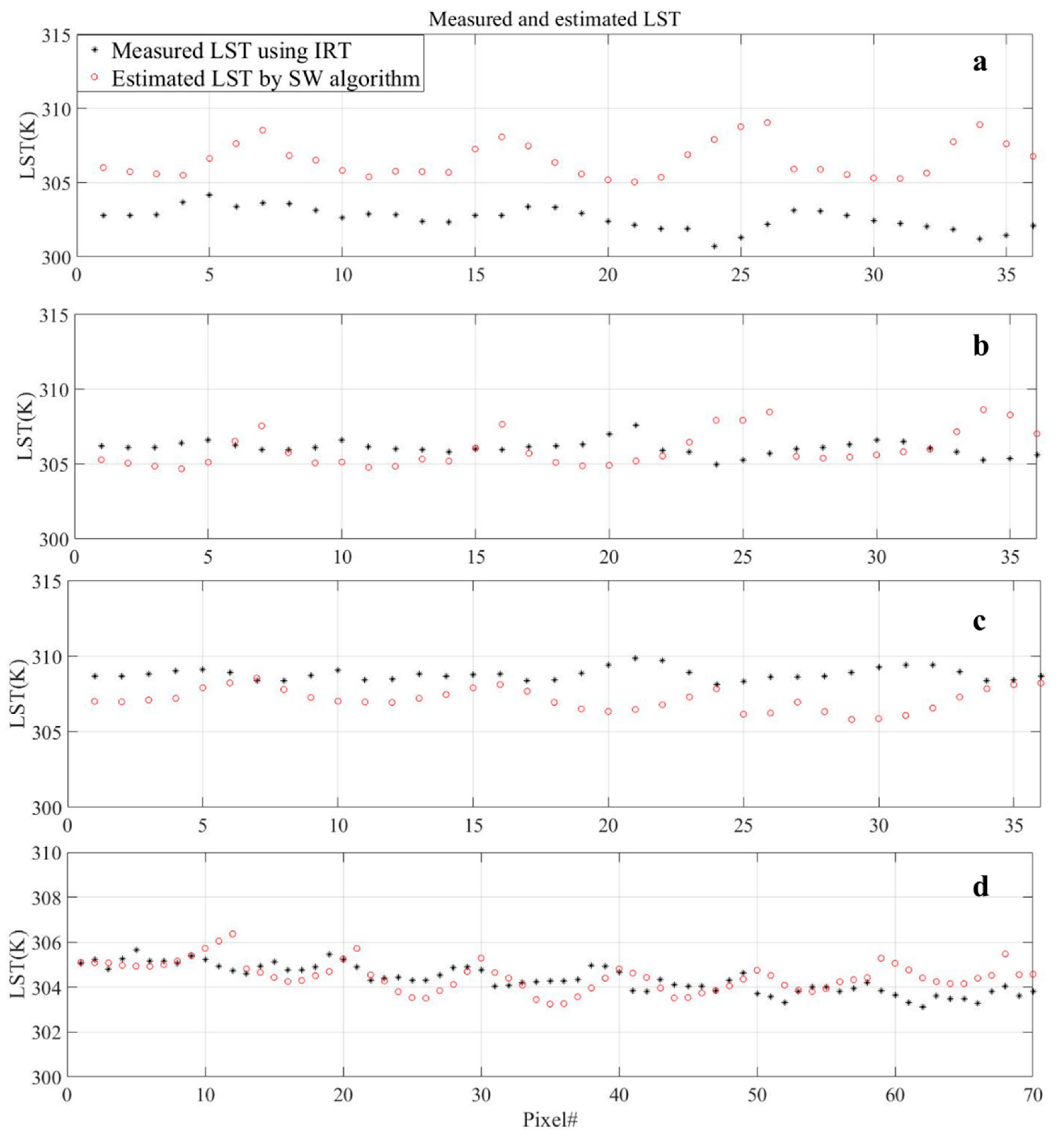
2.6. Validation of LST Retrieval

For calculating LST several parameters, namely LSE, NDVI, brightness temperature (BT) and atmospheric transmittance (τ_i) need to be estimated. The validation was carried out with ground measurements during the time period of satellite overpass. In this regard, leaf surface temperature was measured in 10 points during the overpass to validate the LST product of Landsat 8 which is a continuous raster file, whereas the measured points are discrete value. For selecting the best interpolation method for interpolating the raster surface, nearest neighbor (nn), inverse distance weighting (IDW), spline, and kriging models were tested. Ten observed data were divided into a calibrating set of 7 points and validation data set of 3 points. In this regard, interpolation methods were evaluated by the coefficient of determination (R²) and the root mean square error (RMSE) Equations (20) and (21):

$$R^2=1-\frac{{\sum }_{i=1}^n{(y_i-{\widehat{y}}_i)}^2}{{\sum }_{i=1}^n{(y_i-\overline{y})}^2},$$

(20)

$$RMSE=\sqrt{\sum {(y_i-{\widehat{y}}_i)}^2/n,}$$

(21)

where $y_i$, $\overline{y}$, and ${\widehat{y}}_i$ are observed, average of observed and interpolated temperature at point i, respectively. Moreover, the algorithm is developed for different locations (2 orchards) and time (4 individual dates).

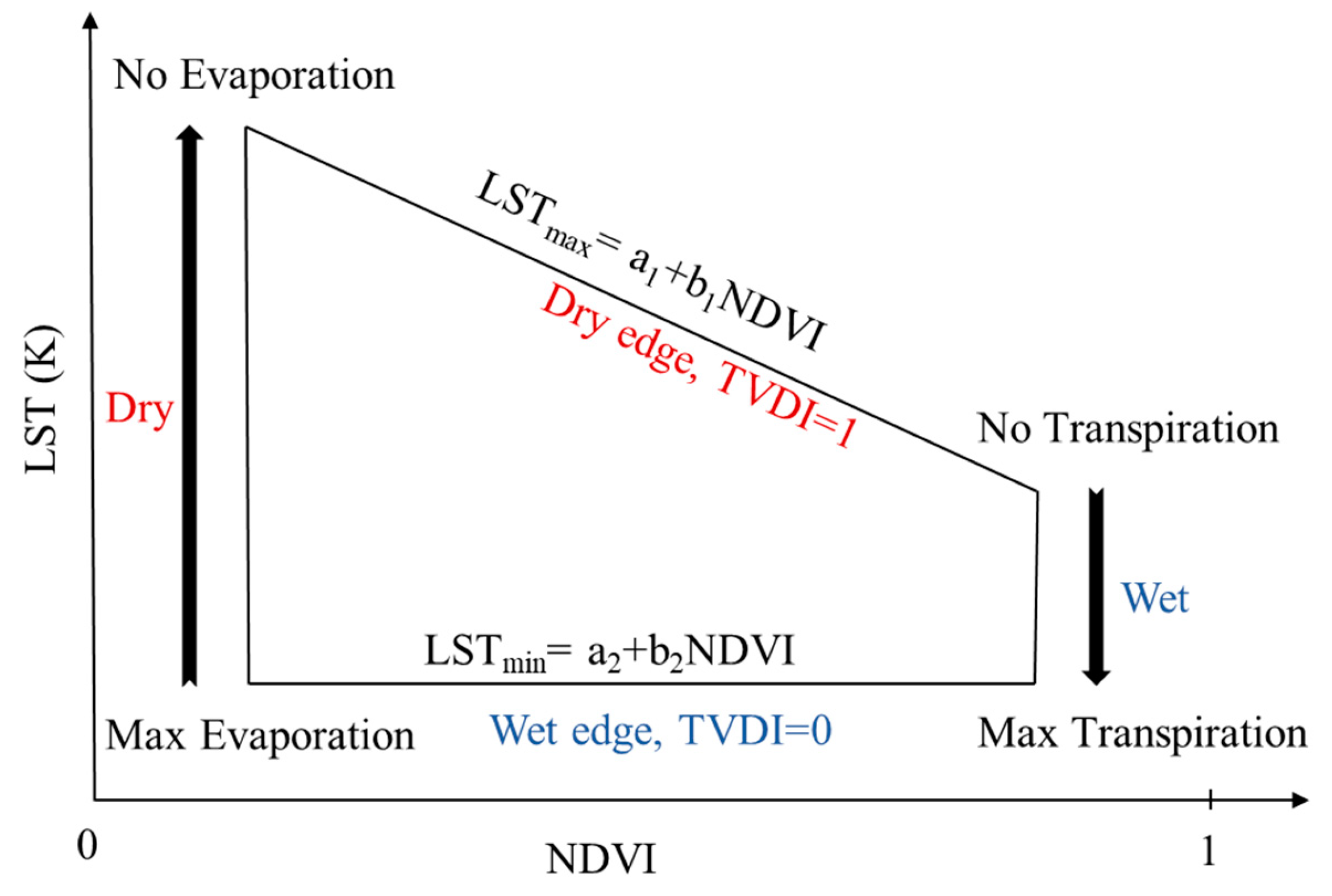
2.7. LST-NDVI Space and TVDI Calculation

The scatter plot of LST and NDVI results in a trapezoidal space [29,47,48]. As Figure 3 shows, each part of this space shows information about canopy water status and soil moisture i.e., the dry and wet edges can be applied to obtain information about water status of the orchard. In the dry edge, a strong negative correlation can be seen between NDVI and LST which shows the water stress condition has been taken place, whereas in the wet edge, the tree is not under stress condition. The TVDI [0;1] is defined by:

$$TVD{I}_i=\frac{LS{T}_i-LS{T}_{min}}{(a_1+b_{1}NDVI)-(a_2+b_{2}NDVI)}=\frac{LS{T}_i-LS{T}_{min}}{LS{T}_{max}-LS{T}_{min}},$$

(22)

where a₁ and b₁ are the intercept and slope of dry edge line (Figure 3), i is the pixel number.

As Figure 3 shows, for TVDI calculation, the NDVI spans from 0 to 1, whereas the range in an apple orchard is limited between 0.2 and 0.7 (Figure 4). Moreover, each point in the trapezoidal space is related to one pixel capturing an area of 900 m², thus an orchard with area less than 10 ha is not big enough to make a trapezoidal space. In this regard, the calculations were done for the whole area of a Landsat 8 satellite image and subsequently, the orchard was extracted.

To calculate the dry and wet edges, the NDVI values were divided into 10 equidistant classes. For each class, the mean value of NDVI is considered as an independent variable of the linear regression, whereas the maximum and minimum values of LST for each class are considered as depended variable for dry and wet regression lines, respectively.

3. Results and Discussion

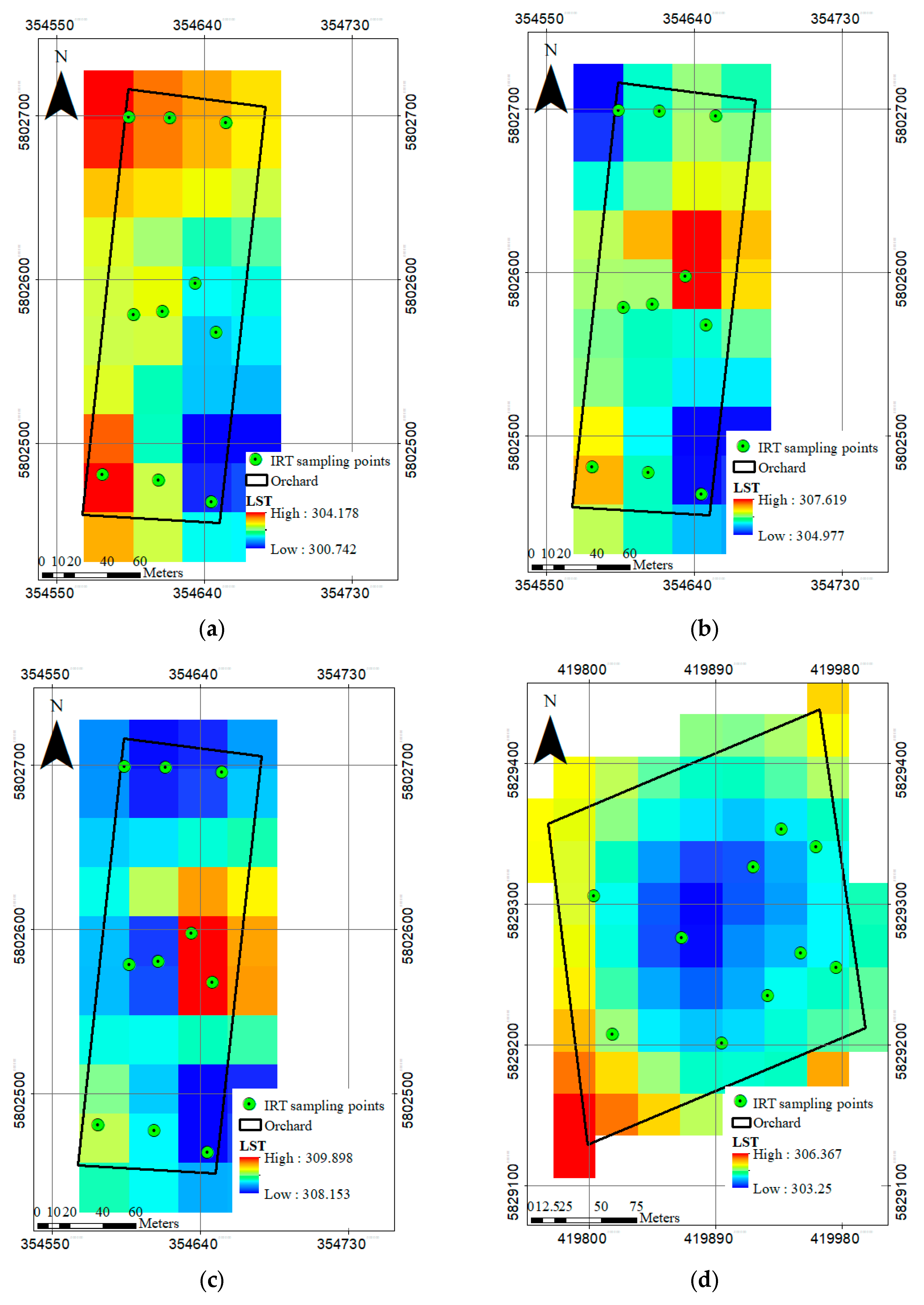
3.1. Interpolation Methods to Generate LST Spatial Distribution Using IRT Ground Measurements

In order to create spatially continuous surfaces data for the LST layer using IRTs measurements, spatial interpolations were conducted. The interpolation exercise according to (a) ordinary kriging, (b) spline (Theissen and regularized method), (c) inverse distance weighting (IDW), and (d) nearest neighbor (nn) pointed out the highest accuracy of the IDW method compared to remaining interpolation methods (

Table 4. Evaluation of interpolation models built on the data set of Glindow apple orchard in 2018 using 7 observed data for calibration and 3 data sets for cross validation. (The red ones are related to selected method).

Date	Index	Calibration				Validation
		Kriging	Spline	IDW	nn	Kriging	Spline	IDW	nn
7 July	RMSE	0.25	0.27	0.21	0.29	0.44	0.40	0.35	0.49
	R2	0.98	0.96	0.98	0.98	0.87	0.87	0.91	0.84
23 July	RMSE	1.02	0.54	0.34	0.38	1.09	1.18	0.61	0.80
	R2	NaN 1	0.81	0.92	0.97	0.00	0.21	0.77	0.54
8 August	RMSE	0.82	0.31	0.34	0.27	1.24	0.82	0.59	0.91
	R2	NaN 1	0.86	0.89	0.95	NaN 1	0.47	0.88	0.37

¹ Not a Number.

) with RMSE 0.21 K and 0.35 K with R² of 0.98 and 0.91 for calibration and cross validation on 7 July 2018 Landsat overpass, respectively. The methods were tested for Glindow and the best method—the IDW—was applied to the Altlandsberg data, as well (Figure 5).

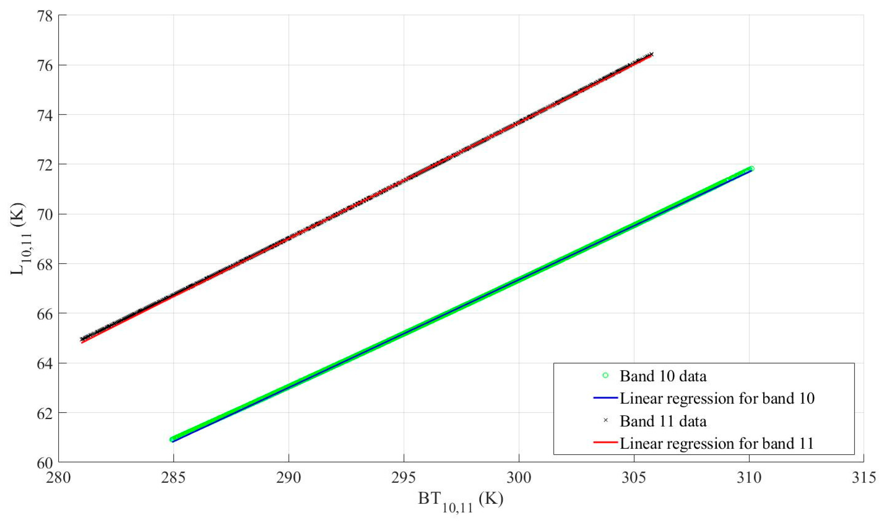
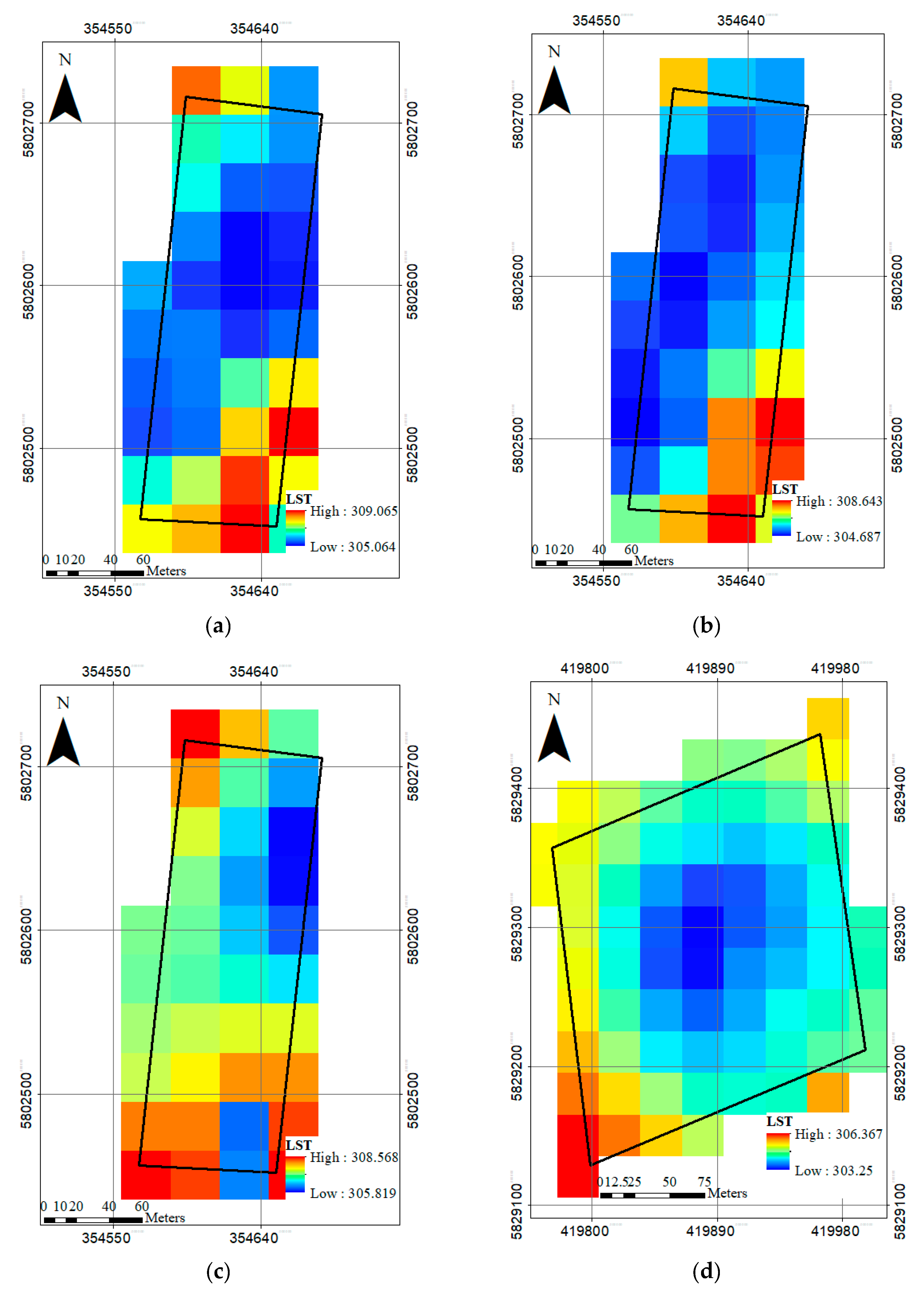
3.2. Split Window (SW) Algorithm to Calculate the LST Spatial Distribution Using Landsat 8 Satellite Images

In order to calculate the satellite-based LST using split window method, the atmospheric transmittance (${\tau }_i$) for bands 10 and 11of Landsat 8 was calculated (

Table 5. Atmospheric transmittance factor (τ_i) for bands 10, 11 of Landsat 8 using water vapor content, w (g/cm²) data.

Date	Location	w (g/cm2)	${\mathit{\tau }}_{\mathbf{10}}$	${\mathit{\tau }}_{\mathbf{11}}$
07-July-18	Glindow	1.5225	0.8695	0.8202
23-July-18	Glindow	1.0232	0.9113	0.8723
08-August-18	Glindow	1.1316	0.9029	0.8615
17-August-18	Altlandsberg	2.1358	0.8069	0.7478

). It was found that the water vapor content (w) appeared in the range of 0.2–3.0 (g/cm²) in all overpasses. As expected by increasing w, the ${\tau }_i$ values are decreased which shows the impact of water particles on the absorption of infrared radiances measured at the thermal bands of Landsat 8 images.

The NDVI was used for estimation of proportion of vegetation $(P_v)$ and LSE. The mean value of $P_v$ for all overpasses was less than 1 ($\overline{P_v}$ ≅ 0.5) which marks that the orchards were not fully covered by trees canopies, thus, the LSE data should be between a percentage of LSE for bare soil and a complementary percentage of tree canopy. The value of NDVI on 7 and 23 July in Glindow is unchanged but a reduction can be seen on 8 August, whereas, no huge difference appeared between vegetation cover in these 3 dates (Figure 4). Consequently, it was expected that the NDVI values would be enhanced or similar to the values on 23 July because the leaf area of tree remains unchanged during this short time interval (23 July to 8 August), while the leaf surface and angle is assumed to change due to the water deficit. Consequently, the high temperature (Tmax = 49.5 °C) and low RH caused reduced NDVI values.

The LSE is one of indispensable inputs for LST estimation models. In the present study, the NBEM method was applied for LSE estimation, which is based on NDVI thresholds for bare soil (NDVI = 0.2) and dense vegetation cover (NDVI = 0.5). The mean value for surface emissivity was 0.98 in all overpasses (

Table 6. Calculated land surface emissivity (LSE) for all Landsat 8 overpasses.

Date	Location	$\mathit{L}\mathit{S}{\mathit{E}}_{\mathit{m}\mathit{i}\mathit{n}}$	$\mathit{L}\mathit{S}{\mathit{E}}_{\mathit{m}\mathit{e}\mathit{a}\mathit{n}}$	$\mathit{L}\mathit{S}{\mathit{E}}_{\mathit{m}\mathit{a}\mathit{x}}$
07-July-18	Glindow	0.9730	0.9775	0.9904
23-July-18	Glindow	0.9730	0.9774	0.9898
08-August-18	Glindow	0.9790	0.9882	0.9912
17-August-18	Altlandsberg	0.9730	0.9731	0.9779

), which means for equal LST, the radiance emitted from orchard surface is 0.02 less than black body surface which is similar to the results of [49].

$a_i$ and $b_i$ in Equation (15) can be estimated by linear regression between $Li$ and $B{T}_i.$ As Figure 6 and

Table 7. Linear regression equations between intermediate parameter $(Li)$ and top of atmosphere brightness temperature $(B{T}_i)$, $i=10,11$ to determine $a_i$ and $b_i$ coefficients for thermal bands of Landsat 8 satellite.

Date	Location	${\mathit{L}}_{\mathbf{10}}\mathbf{=}{\mathit{a}}_{\mathbf{10}}\mathbf{+}{\mathit{b}}_{\mathbf{10}}\mathbf{\ast }\mathit{B}{\mathit{T}}_{\mathbf{10}}$	${\mathit{L}}_{\mathbf{11}}\mathbf{=}{\mathit{a}}_{\mathbf{11}}\mathbf{+}{\mathit{b}}_{\mathbf{11}}\mathbf{\ast }\mathit{B}{\mathit{T}}_{\mathbf{11}}$
07-July-18	Glindow	$L_{10}=-62.96+0.43\ast B{T}_{10}$	$L_{11}=-66.41+0.47\ast B{T}_{11}$
23-July-18	Glindow	$L_{10}=-63.88+0.44\ast B{T}_{10}$	$L_{11}=-67.35+0.47\ast B{T}_{11}$
08-August-18	Glindow	$L_{10}=-61.74+0.43\ast B{T}_{10}$	$L_{11}=-64.75+0.46\ast B{T}_{11}$
17-August-18	Altlandsberg	$L_{10}=-64.37+0.44\ast B{T}_{10}$	$L_{11}=-67.55+0.47\ast B{T}_{11}$

show, the $a_i$ coefficients are between −64.37 and −61.74 for bands 10 and 11, respectively whereas, the $b_i$ coefficients are about 0.45 for both thermal bands. The data were perfectly fitted to the regression line (Figure 6) in all overpasses (R² = 1).

By calculating all required parameters and coefficients, the spatial distribution of LST was estimated by SW method. As Figure 7 shows, the lower temperatures are assigned to the pixels with enhanced NDVI.

To validate SW Landsat 8 LST retrieval, IRT observations were applied. As Figure 8 and

Table 8. The mean errors and root mean square error (RMSE) for comparison between measured land surface temperature (LST) using infrared thermometers(IRT) and split window (SW) satellite-based LST in Kelvin (K).

Date	Location	Mean Error (K)	RMSE (K)
07-July-18	Glindow	−3.94	4.23
23-July-18	Glindow	0.08	1.55
08-August-18	Glindow	1.68	1.93
17-August-18	Altlandsberg	−0.12	0.71

show, the absolute mean error of the SW method was below 4 K in all overpasses to the extent that the maximum RMSE was found on 7 July with the value of 4.23 K and absolute mean error of 3.94 K. On the other hand, the RMSE value on the 17 August overpass in Altlandsberg was only 0.71 K with absolute mean error of 0.12 K.

The reason for errors can be related to the very dynamic nature of LST e.g., the variation of 10 K has been reported in few centimeters or 1 K change were taken place in 1 min [50]. As indicated in pervious parts, the ground measurements were done during the satellite transit time over the orchards to minimize these variations. All above shows that estimating the LST with 0.08–4 K error using open access satellite images is accurate enough for water status studies. It is important to note that the IDW interpolation method as well as the SW model were developed for Glindow orchard on 7 July 2018, and then applied for different dates in Glindow and Altlandsberg, as well. i.e., the application of models was validated temporally and spatially. The results proved that both models (IDW and SW) can be used for different time and location.

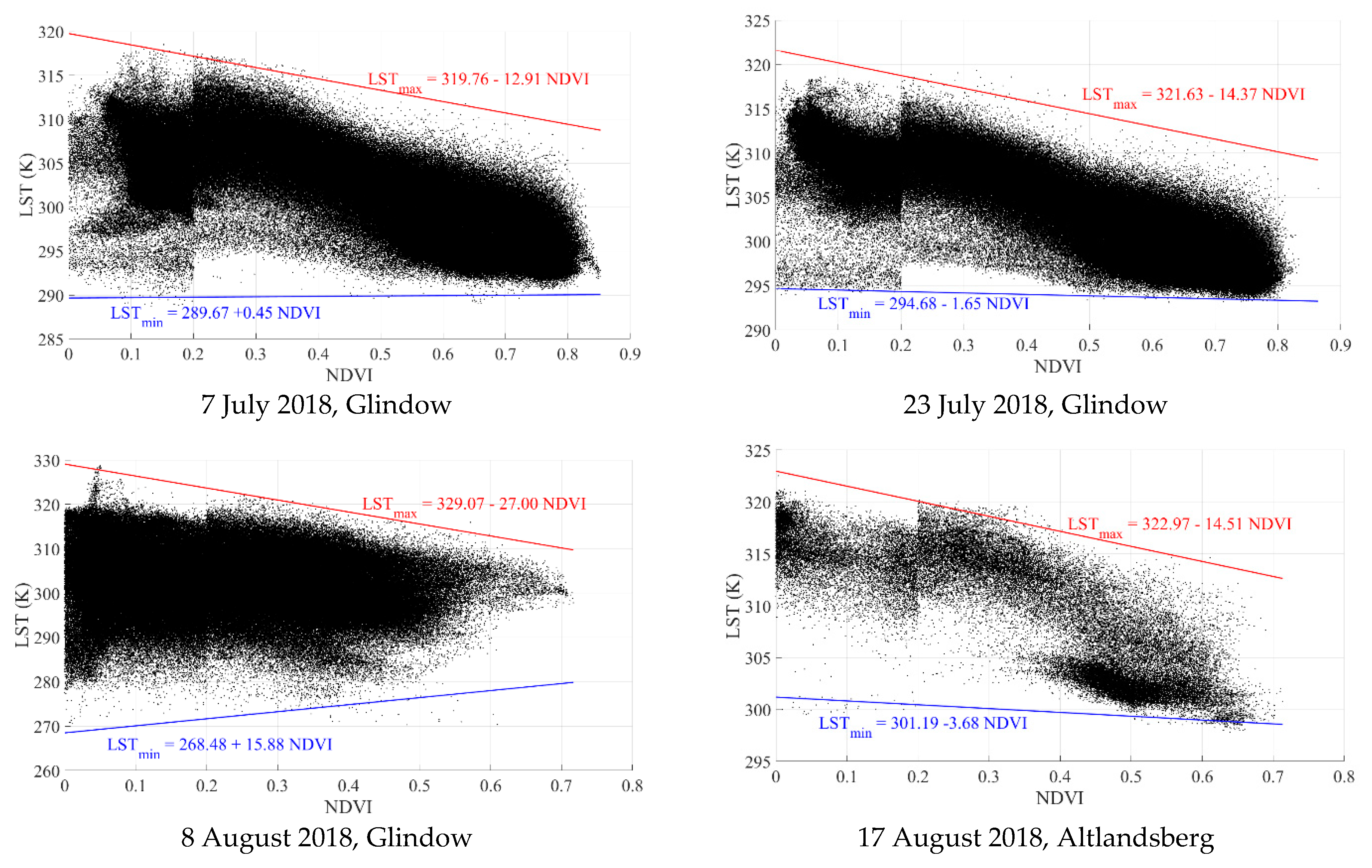
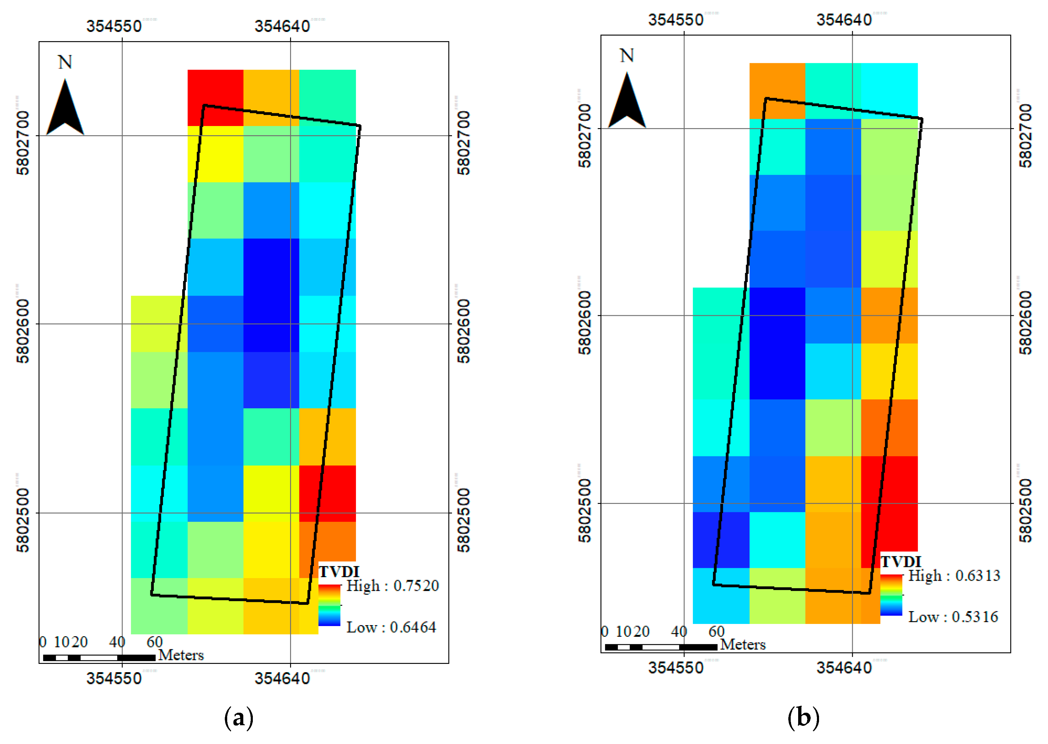
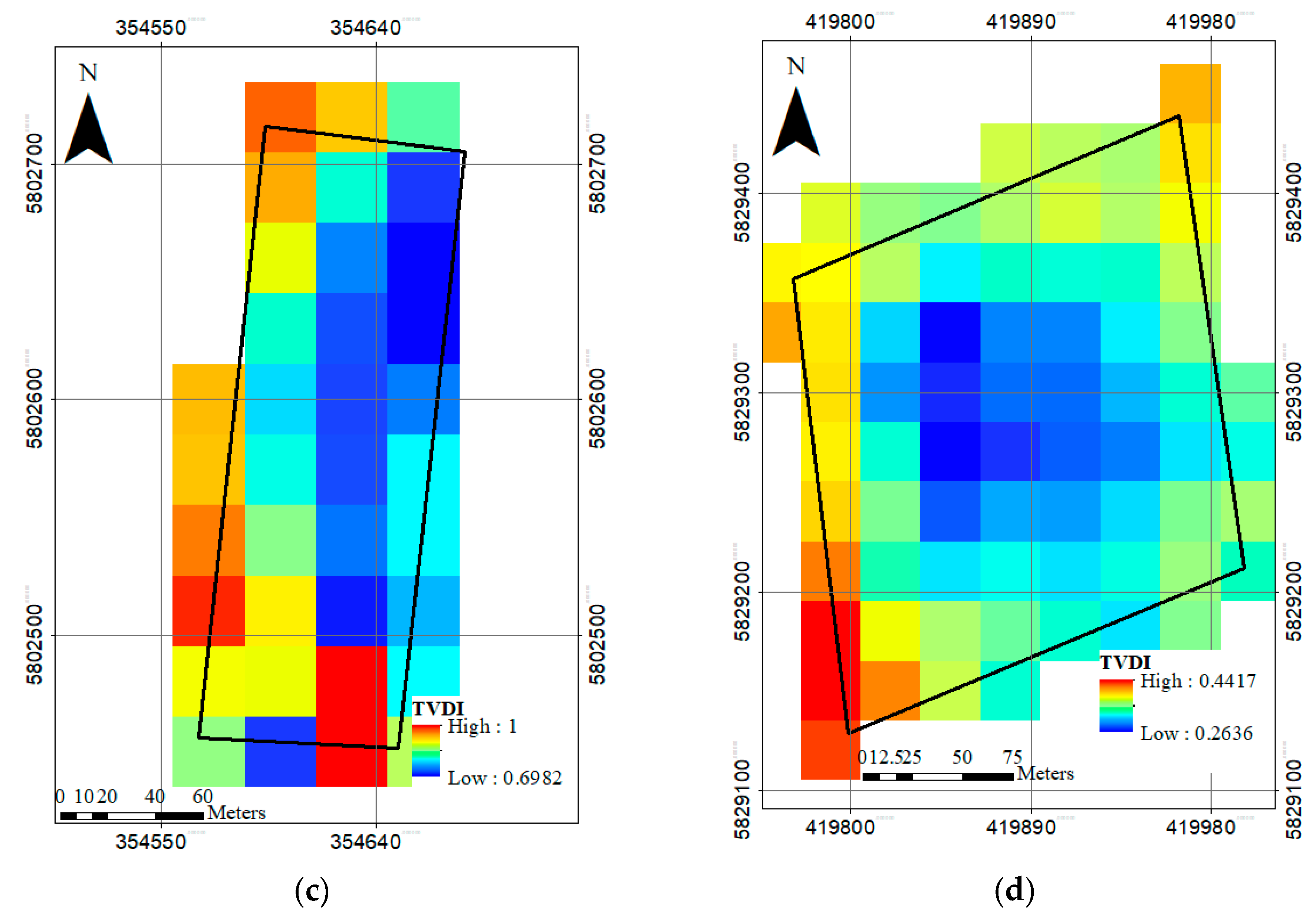
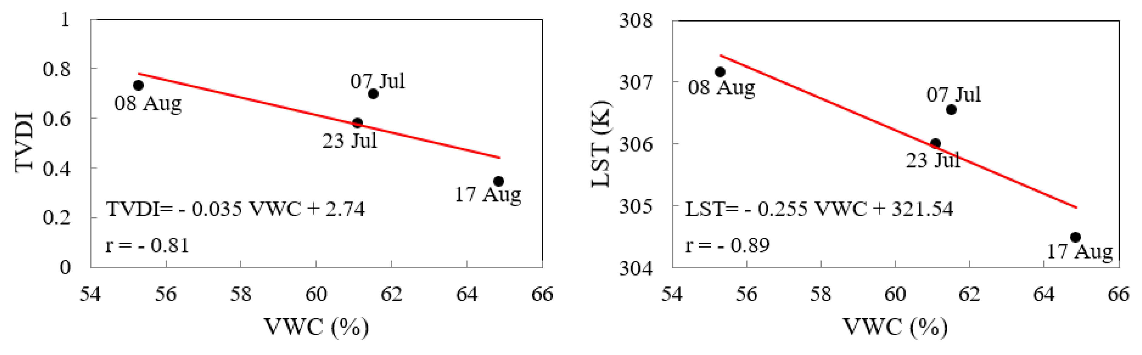
3.3. LST-NDVI Trapezoidal Space for TVDI Calculation

In the next step, the equations of dry and wet edges of trapezoidal space between LST and NDVI were determined by linear regression model. The maximum and minimum values of LST for NDVI value can be used for dry and wet lines’ equation using linear regression (Figure 9). By using these equations, the TVDI can be estimated. The effects of land surface emissivity (LSE) and proportion of vegetation $(P_v)$ on LST calculation can be clearly seen in Figure 9 where data went up at NDVI = 0.2 (NDVI value for bare soil).

As indicated in the material and methods part, in the TVDI calculations, two visible bands (NIR and red) and TIRS bands of Landsat 8 are applied. In this regard, the dry and wet edges of LST/NDVI space were defined by using Equation (22), the spatial distribution of TVDI were generated (Figure 10). The mean values of TVDI on 7 and 23 July in Glindow are 0.69 and 0.57 which show the trees are under moderate water stress and the irrigation system should start to work soon but on 8 August—as expected—the trees are under severe water stress where the mean TVDI is 0.73; therefore, the irrigation system was not working at the appropriate time and needs to start irrigation immediately. On the other hand, the drip irrigation in the Altlandsberg orchard already started to work during the measurements as well the satellite overpass, and it can be seen the TVDI is less than 0.5 (averagely 0.34), so the tree water status is in normal condition without water stress.

As spatial distribution of TVDI pointed to low values in the center of the orchard and maximum values near the sides of the field on 7, 23 July 2018 in Glindow and 17 August 2018 in Altlandsberg. Here the effects of non-vegetated areas like roads and bare soils in side pixels became visible. Although the minimum values of TVDI on 8 August took place in the central pixel as well, the spatial distribution did not follow a trend like others which can be related to the high weather temperature and low relative humidity that cause an intensive dryness in the whole area without considering the land cover. The minimum value of TVDI is already equal to 0.7 which shows severe dryness.

The results illustrated that, the LST and TVDI can be applied as indicators for vegetation water content (VWC), thus the correlation between latter parameters was investigated. In order to find the relation between VWC and TVDI (and/or LST), and more importantly to validate the satellite based index, a linear regression model was developed between two parameters. As Figure 11 shows, the empirical relationship between values of measured VWC and TVDI/LST has a relatively high negative correlation coefficient. Relationships between VWC and temperature-based indices for different trees at different locations would enable irrigation planners to estimate VWC.

The accuracy of the SW satellite-based algorithm was evaluated in studies published in the literature (e.g., [22]) which is one of main goals of the present study as well; however, it is notable to say in the case of this study, the data evaluated by ground measured data in the same time of the Landsat 8 overpass. Moreover, many studies applying satellite imagery for water status estimation based on land surface temperature (LST) were carried out in relatively large field crops (e.g., [47]), whereas, the application in apple orchards were investigated in this study. It is important to note the code of the TVDI calculation using Landsat 8 images is available on GitHub [51], the strong point of the provided algorithm is by introducing the satellite images as input to the code, several outputs including NDVI, LST, and TVDI spatial distribution maps can be obtained by the user.

4. Conclusions

In this study, progress has been made in combining the advantage of available open access Landsat 8 satellite images with scientific advances to estimate tree water status in apple orchards. In this regard, the TDVI was derived from land surface temperature and NDVI outlining the spatial distribution of tree water status illustrating that the satellite-based data can provide an alternative to the manual temperature readings and vegetation water content with values of absolute mean error ranging from 0.08 to 3.94 K and RMSE of 0.71 to 4.23 K between satellite-based estimated LST and measured canopy temperature for all overpasses. Moreover, the relationship between vegetation water content and TVDI (and LST) with r = −0.81 (and −0.89). It is concluded that the satellite-based methods for determining the LST, and subsequently TVDI provides advantages over ground measurements methods, because the ground observed LST are point data whereas the spatial and temporal LST changes are very dynamic. Therefore, it can be assumed that calculating the spatial distribution of LST pixel by pixel is more reliable than using interpolation methods from limited discrete point measurement. In addition, the vegetation water content can be revealed by estimated LST and TVDI, derived from thermal images for water stress detection. The remote sensing method outperforms time-consuming sampling of a large number of IRT measurements in the field. Consequently, the TVDI index using thermal bands of Landsat 8 has the potential to replace direct vegetation water content measurements and to provide a more robust measure of the tree water status and its spatial patterns of the apple production. Moreover, it can be an efficient parameter for land use change detection in mesoscale studies as well as irrigation water management planning projects.

References

1. Qamar uz, Z.; Schumann, A.W. Nutrient management zones for citrus based on variation in soil properties and tree performance. Precis. Agric. 2006, 7, 45–63. [Google Scholar] [CrossRef]
2. Zude-Sasse, M.; Fountas, S.; Gemtos, T.A.; Abu-Khalaf, N. Applications of precision agriculture in horticultural crops. Eur. J. Hortic. Sci. 2016, 81, 78–90. [Google Scholar] [CrossRef]
3. Allen, R.G.; Pereira, L.S.; Raes, D.; Smith, M. Crop Evapotranspiration-Guidelines for Computing Crop Water Requirements-FAO Irrigation and Drainage Paper 56; FAO: Rome, Italy, 1998; Volume 300, p. D05109. [Google Scholar]
4. Allen Richard, G.; Tasumi, M.; Morse, A.; Trezza, R.; Wright James, L.; Bastiaanssen, W.; Kramber, W.; Lorite, I.; Robison Clarence, W. Satellite-based energy balance for mapping evapotranspiration with internalized calibration (metric)—Applications. J. Irrig. Drain. Eng. 2007, 133, 395–406. [Google Scholar] [CrossRef]
5. Berni, J.A.J.; Zarco-Tejada, P.J.; Sepulcre-Cantó, G.; Fereres, E.; Villalobos, F. Mapping canopy conductance and cwsi in olive orchards using high resolution thermal remote sensing imagery. Remote Sens. Environ. 2009, 113, 2380–2388. [Google Scholar] [CrossRef]
6. Zare, M.; Koch, M. Computation of the irrigation water demand in the miandarband plain, iran, using fao-56- and satellite- estimated crop coefficients. J. Thai Interdiscip. Res. 2016, 12, 10. [Google Scholar]
7. Ben-Gal, A.; Agam, N.; Alchanatis, V.; Cohen, Y.; Yermiyahu, U.; Zipori, I.; Presnov, E.; Sprintsin, M.; Dag, A. Evaluating water stress in irrigated olives: Correlation of soil water status, tree water status, and thermal imagery. Irrig. Sci. 2009, 27, 367–376. [Google Scholar] [CrossRef]
8. Agam, N.; Segal, E.; Peeters, A.; Levi, A.; Dag, A.; Yermiyahu, U.; Ben-Gal, A. Spatial distribution of water status in irrigated olive orchards by thermal imaging. Precis. Agric. 2014, 15, 346–359. [Google Scholar] [CrossRef]
9. Bellvert, J.; Zarco-Tejada, P.J.; Girona, J.; Fereres, E. Mapping crop water stress index in a ‘pinot-noir’ vineyard: Comparing ground measurements with thermal remote sensing imagery from an unmanned aerial vehicle. Precis. Agric. 2014, 15, 361–376. [Google Scholar] [CrossRef]
10. Drastig, K.; Prochnow, A.; Libra, J.; Koch, H.; Rolinski, S. Irrigation water demand of selected agricultural crops in germany between 1902 and 2010. Sci. Total Environ. 2016, 569–570, 1299–1314. [Google Scholar] [CrossRef]
11. Käthner, J.; Ben-Gal, A.; Gebbers, R.; Peeters, A.; Herppich, W.B.; Zude-Sasse, M. Evaluating spatially resolved influence of soil and tree water status on quality of european plum grown in semi-humid climate. Front. Plant Sci. 2017, 8, 1053. [Google Scholar] [CrossRef] [PubMed] [Green Version]
12. Baroni, G.; Drastig, K.; Lichtenfeld, A.U.; Jost, L.; Claas, P. Assessment of irrigation scheduling systems in germany: Survey of the users and comparative study. Irrig. Drain. 2019, 68, 520–530. [Google Scholar] [CrossRef]
13. Naor, A.; Hupert, H.; Greenblat, Y.; Peres, M.; Kaufman, A.; Klein, I. The response of nectarine fruit size and midday stem water potential to irrigation level in stage iii and crop load. J. Am. Soc. Hortic. Sci. 2001, 126, 140–143. [Google Scholar] [CrossRef] [Green Version]
14. Geerts, S.; Raes, D. Deficit irrigation as an on-farm strategy to maximize crop water productivity in dry areas. Agric. Water Manag. 2009, 96, 1275–1284. [Google Scholar] [CrossRef] [Green Version]
15. Mahan, J.R.; Young, A.W.; Payton, P. Deficit irrigation in a production setting: Canopy temperature as an adjunct to et estimates. Irrig. Sci. 2012, 30, 127–137. [Google Scholar] [CrossRef]
16. Jones, H.G. Plants and Microclimate: A Quantitative Approach to Environmental Plant Physiology; Cambridge University Press: Melbourne, Australia, 1992. [Google Scholar]
17. Sun, D.; Pinker, R.T. Estimation of land surface temperature from a geostationary operational environmental satellite (goes-8). J. Geophys. Res. Atmos. 2003, 108. [Google Scholar] [CrossRef]
18. Friedel, M.J. Data-driven modeling of surface temperature anomaly and solar activity trends. Environ. Model. Softw. 2012, 37, 217–232. [Google Scholar] [CrossRef]
19. Maimaitiyiming, M.; Ghulam, A.; Tiyip, T.; Pla, F.; Latorre-Carmona, P.; Halik, Ü.; Sawut, M.; Caetano, M. Effects of green space spatial pattern on land surface temperature: Implications for sustainable urban planning and climate change adaptation. ISPRS J. Photogramm. Remote Sens. 2014, 89, 59–66. [Google Scholar] [CrossRef] [Green Version]
20. Price, J.C. Land surface temperature measurements from the split window channels of the noaa 7 advanced very high resolution radiometer. J. Geophys. Res. Atmos. 1984, 89, 7231–7237. [Google Scholar] [CrossRef]
21. Veysi, S.; Naseri, A.A.; Hamzeh, S.; Bartholomeus, H. A satellite based crop water stress index for irrigation scheduling in sugarcane fields. Agric. Water Manag. 2017, 189, 70–86. [Google Scholar] [CrossRef]
22. Nikam, B.R.; Ibragimov, F.; Chouksey, A.; Garg, V.; Aggarwal, S.P. Retrieval of land surface temperature from landsat 8 tirs for the command area of mula irrigation project. Environ. Earth Sci. 2016, 75, 1169. [Google Scholar] [CrossRef]
23. Sheng, J.; Wilson, J.P.; Lee, S. Comparison of land surface temperature (lst) modeled with a spatially-distributed solar radiation model (srad) and remote sensing data. Environ. Model. Softw. 2009, 24, 436–443. [Google Scholar] [CrossRef]
24. Tan, K.; Liao, Z.; Du, P.; Wu, L. Land surface temperature retrieval from Landsat 8 data and validation with geosensor network. Front. Earth Sci. 2017, 11, 20–34. [Google Scholar] [CrossRef]
25. Yang, J.; Wang, Y. Estimating evapotranspiration fraction by modeling two-dimensional space of ndvi/albedo and day-night land surface temperature difference: A comparative study. Adv. Water Resour. 2011, 34, 512–518. [Google Scholar] [CrossRef]
26. García-Santos, V.; Cuxart, J.; Martínez-Villagrasa, D.; Jiménez, A.M.; Simó, G. Comparison of three methods for estimating land surface temperature from landsat 8-tirs sensor data. Remote Sens. 2018, 10, 1450. [Google Scholar] [CrossRef] [Green Version]
27. Yi, Q.X.; Bao, A.M.; Wang, Q.; Zhao, J. Estimation of leaf water content in cotton by means of hyperspectral indices. Comput. Electron. Agric. 2013, 90, 144–151. [Google Scholar] [CrossRef]
28. Long, D.; Singh, V.P. A two-source trapezoid model for evapotranspiration (ttme) from satellite imagery. Remote Sens. Environ. 2012, 121, 370–388. [Google Scholar] [CrossRef]
29. Sandholt, I.; Rasmussen, K.; Andersen, J. A simple interpretation of the surface temperature/vegetation index space for assessment of surface moisture status. Remote Sens. Environ. 2002, 79, 213–224. [Google Scholar] [CrossRef]
30. Jiménez-Muñoz, J.C.; Sobrino, J.A.; Skoković, D.; Mattar, C.; Cristóbal, J. Land surface temperature retrieval methods from landsat-8 thermal infrared sensor data. IEEE Geosci. Remote Sens. Lett. 2014, 11, 1840–1843. [Google Scholar] [CrossRef]
31. Yang, L.; Cao, Y.; Zhu, X.; Zeng, S.; Yang, G.; He, J.; Yang, X. Land surface temperature retrieval for arid regions based on landsat-8 tirs data: A case study in shihezi, northwest china. J. Arid Land 2014, 6, 704–716. [Google Scholar] [CrossRef] [Green Version]
32. USGS. Landsat 8 (L8) Data Users Handbook, Version 2.0; Department of the Interior, USGS: Sioux Falls, SD, USA, 2016; p. 98.
33. Tucker, C.J. Red and photographic infrared linear combinations for monitoring vegetation. Remote Sens. Environ. 1979, 8, 127–150. [Google Scholar] [CrossRef] [Green Version]
34. Ozelkan, E.; Chen, G.; Ustundag, B.B. Multiscale object-based drought monitoring and comparison in rainfed and irrigated agriculture from landsat 8 oli imagery. Int. J. Appl. Earth Obs. Geoinf. 2016, 44, 159–170. [Google Scholar] [CrossRef]
35. Mao, K.; Qin, Z.; Shi, J.; Gong, P. A practical split-window algorithm for retrieving land-surface temperature from modis data. Int. J. Remote Sens. 2005, 26, 3181–3204. [Google Scholar] [CrossRef]
36. Yu, X.; Guo, X.; Wu, Z. Land surface temperature retrieval from landsat 8 tirs—Comparison between radiative transfer equation-based method, split window algorithm and single channel method. Remote Sens. 2014, 6, 9829–9852. [Google Scholar] [CrossRef] [Green Version]
37. Qin, Z.; Karnieli, A.; Berliner, P. A mono-window algorithm for retrieving land surface temperature from landsat tm data and its application to the israel-egypt border region. Int. J. Remote Sens. 2001, 22, 3719–3746. [Google Scholar] [CrossRef]
38. Rozenstein, O.; Qin, Z.; Derimian, Y.; Karnieli, A. Derivation of land surface temperature for landsat-8 tirs using a split window algorithm. Sensors 2014, 14, 5768–5780. [Google Scholar] [CrossRef] [PubMed]
39. Rozenstein, O.; Qin, Z.; Derimian, Y.; Karnieli, A. Correction: Rozenstein, o., et al. Derivation of land surface temperature for landsat-8 tirs using a split window algorithm. Sensors 2014, 14, 5768–5780. Sensors 2014, 14, 11277. [Google Scholar] [CrossRef] [Green Version]
40. Qin, Z.; Zhang, M.; Karnieli, A. Split window algorithms for retrieving land surface temperature from noaa-avhrr data. Remote Sens. Land Resour. 2001, 13, 33–42. [Google Scholar]
41. Allen, R.; Tasumi, M.; Trezza, R.; Bastiaanssen, W. Sebal (surface energy balance algorithms for land). Adv. Train. Users Man. IDA Implement. Version 2002, 1, 97. [Google Scholar]
42. Li, Z.L.; Wu, H.; Wang, N.; Qiu, S.; Sobrino, J.A.; Wan, Z.; Tang, B.H.; Yan, G. Land surface emissivity retrieval from satellite data. Int. J. Remote Sens. 2013, 34, 3084–3127. [Google Scholar] [CrossRef]
43. Sobrino, J.A.; Jiménez-Muñoz, J.C.; Paolini, L. Land surface temperature retrieval from landsat tm 5. Remote Sens. Environ. 2004, 90, 434–440. [Google Scholar] [CrossRef]
44. Wang, F.; Qin, Z.; Song, C.; Tu, L.; Karnieli, A.; Zhao, S. An improved mono-window algorithm for land surface temperature retrieval from landsat 8 thermal infrared sensor data. Remote Sens. 2015, 7, 4268–4289. [Google Scholar] [CrossRef] [Green Version]
45. Sánchez, J.M.; Scavone, G.; Caselles, V.; Valor, E.; Copertino, V.A.; Telesca, V. Monitoring daily evapotranspiration at a regional scale from landsat-tm and etm+ data: Application to the basilicata region. J. Hydrol. 2008, 351, 58–70. [Google Scholar] [CrossRef]
46. Qin, Z.; Dall’Olmo, G.; Karnieli, A.; Berliner, P. Derivation of split window algorithm and its sensitivity analysis for retrieving land surface temperature from noaa-advanced very high resolution radiometer data. J. Geophys. Res. Atmos. 2001, 106, 22655–22670. [Google Scholar] [CrossRef]
47. Abuzar, M.; O’Leary, G.; Fitzgerald, G. Measuring water stress in a wheat crop on a spatial scale using airborne thermal and multispectral imagery. Field Crop. Res. 2009, 112, 55–65. [Google Scholar] [CrossRef]
48. Zhang, F.; Zhang, L.W.; Shi, J.J.; Huang, J.F. Soil moisture monitoring based on land surface temperature-vegetation index space derived from modis data. Pedosphere 2014, 24, 450–460. [Google Scholar] [CrossRef]
49. Wilber, A.C.; Kratz, D.P.; Gupta, S.K. Surface Emissivity Maps for Use in Satellite Retrievals of Longwave Radiation; NASA Langley Research Center: Hampton, VA, USA, 1999.
50. Prata, A.J.; Caselles, V.; Coll, C.; Sobrino, J.A.; Ottlé, C. Thermal remote sensing of land surface temperature from satellites: Current status and future prospects. Remote Sens. Rev. 1995, 12, 175–224. [Google Scholar] [CrossRef]
51. Zare, M. Calculate Tvdi Using Landsat 8 Images. GitHub Repository: 2019. Available online: https://github.com/ATB-Potsdam/Matlab_TVDI_cal (accessed on 19 December 2019).
Figure 1. The study areas; left panel: Glindow apple orchard with center point of (1) and right panel: Altlandsberg apple orchards with center point of (2).
Sustainability 12 00070 g001
Figure 2. Flowchart of split window (SW) algorithm.
Sustainability 12 00070 g002
Figure 3. Land surface temperature (LST)—NDVI trapezoidal space for temperature vegetation dryness index (TVDI [0;1]) estimation.
Sustainability 12 00070 g003
Figure 4. Spatial distribution of normalized difference vegetation index (NDVI [–1;1]) analyzed using satellite images. (a) 7 July 2018, Glindow; (b) 23 July 2018, Glindow; (c) 8 August 2018, Glindow; (d) 17 August 2018, Altlandsberg.
Sustainability 12 00070 g004
Figure 5. Measuring points of manual reference readings with infrared thermometer (IRT) and the spatial distribution of observed land surface temperature (LST) in Kelvin (K) using inverse distance weighting (IDW) interpolation method. (a) 7 July 2018, Glindow; (b) 23 July 2018, Glindow; (c) 8 August 2018, Glindow; (d) 17 August 2018, Altlandsberg.
Sustainability 12 00070 g005
Figure 6. The linear regression equations between intermediate parameter ( L i ) and top of atmosphere brightness temperature ( B T i ) , i = 10 , 11 for Landsat 8 thermal bands on 7 July 2018, Glindow to determine a i and b i coefficients.
Sustainability 12 00070 g006
Figure 7. The spatial distribution of calculated land surface temperature (LST) using split window (SW) method using Landsat 8 satellite images. (a) 7 July 2018, Glindow; (b) 23 July 2018, Glindow; (c) 8 August 2018, Glindow; (d) 17 August 2018, Altlandsberg.
Sustainability 12 00070 g007
Figure 8. Comparison between inverse distance weighting (IDW) interpolated land surface temperature (LST) using infrared thermometers (IRT) and split window (SW) satellite based LST map on (a) 7 July; (b) 23 July; (c) 8 August 2018 Landsat 8 overpass, Glindow; and (d) on 17 August 2018, Altlandsberg.
Sustainability 12 00070 g008
Figure 9. Trapezoidal space of land surface temperature (LST)/NDVI using Landsat 8 satellite images to calculate temperature vegetation dryness index (TVDI [0;1]). The wet edge (blue line) is the area where TVDI = 0 and the dry edge (red line) is the area with TVDI = 1.
Sustainability 12 00070 g009
Figure 10. Temperature vegetation dryness index (TVDI [0;1]) spatial distribution for apple orchards. (a) 7 July 2018, Glindow; (b) 23 July 2018, Glindow; (c) 8 August 2018, Glindow; (d) 17 August 2018, Altlandsberg.
Sustainability 12 00070 g010aSustainability 12 00070 g010b
Figure 11. Empirical relationship between vegetation water content (VWC) and satellite based indices; left panel: temperature vegetation dryness index (TVDI), right panel: land surface temperature (LST).
Sustainability 12 00070 g011