Technical Note

Climate: An R Package to Access Free In-Situ Meteorological and Hydrological Datasets For Environmental Assessment

by
Bartosz Czernecki
1,
Arkadiusz Głogowski
2,* and
Jakub Nowosad
3
1
Department of Climatology, Faculty of Geographical and Geological Sciences, Adam Mickiewicz University, 61-680 Poznań, Poland
2
Institute of Environmental Protection and Development, Wrocław University of Environmental and Life Sciences, 50-375 Wrocław, Poland
3
Institute of Geoecology and Geoinformation, Faculty of Geographical and Geological Sciences, Adam Mickiewicz University, 61-680 Poznań, Poland
*
Author to whom correspondence should be addressed.
Sustainability 2020, 12(1), 394; https://doi.org/10.3390/su12010394
Submission received: 2 December 2019 / Revised: 25 December 2019 / Accepted: 30 December 2019 / Published: 3 January 2020

Abstract

:
Freely available and reliable meteorological datasets are highly demanded in many scientific and business applications. However, the structure of publicly available databases is often difficult to follow, especially for users who only deal with this kind of dataset on occasion. The “climate” R package aims to fill this gap with an easy-to-use interface for downloading global meteorological data in a fast and consistent way. The package provides access to different sources of in-situ meteorological data, including the Ogimet website, atmospheric vertical sounding gathered at the University of Wyoming’s webpage, and hydrological and meteorological measurements collected by the Institute of Meteorology and Water Management—National Research Institute (i.e., Polish Met Office). This article also provides a quick overview of the key functionalities available within the climate R package, and gives examples of an efficient and tidy workflow of meteorological data within the R based environment. The automation procedures included in the packages allow one to download data in a user-defined time resolution (from hourly to annual), for a user-defined time span, and for a specified group of stations or countries. The package also contains metadata, including a list of available stations, their geospatial information, and measurement descriptions with their units. Finally, the obtained datasets can be processed in R or exported to external tools (e.g., spreadsheets or GIS software).

1. Introduction

Meteorological conditions are key factors in many areas of human activity such as agriculture, transport, power engineering, insurance and risk assessment [1], industrial and marketing planning [2], tourism, sport, mass events [3,4], national security, and many more where atmospheric conditions may have a direct or indirect impact [5,6,7,8]. Besides the financial and safety relevance of meteorological and hydrological datasets [9], this kind of information is very often crucial to reliably answer a scientific problem [10], which heavily relies on the quality of meteorological dataset used in this kind of research.
National meteorological agencies collect in-situ measurements of the highest quality according to the standards of the World Meteorological Organization (WMO). They are simultaneously responsible for maintaining and sharing their archived databases. A significant part of the meteorological data is available for free from the global exchange of the surface synoptic observations (SYNOP), meteorological information used by aircraft pilots (METAR), or upper air soundings (TEMP) reports. Even if most of this information is limited only to the main synoptic stations and covers only basic meteorological parameters, the data itself usually provides better accuracy compared to commonly applied coarse gridded reanalysis products [11,12].
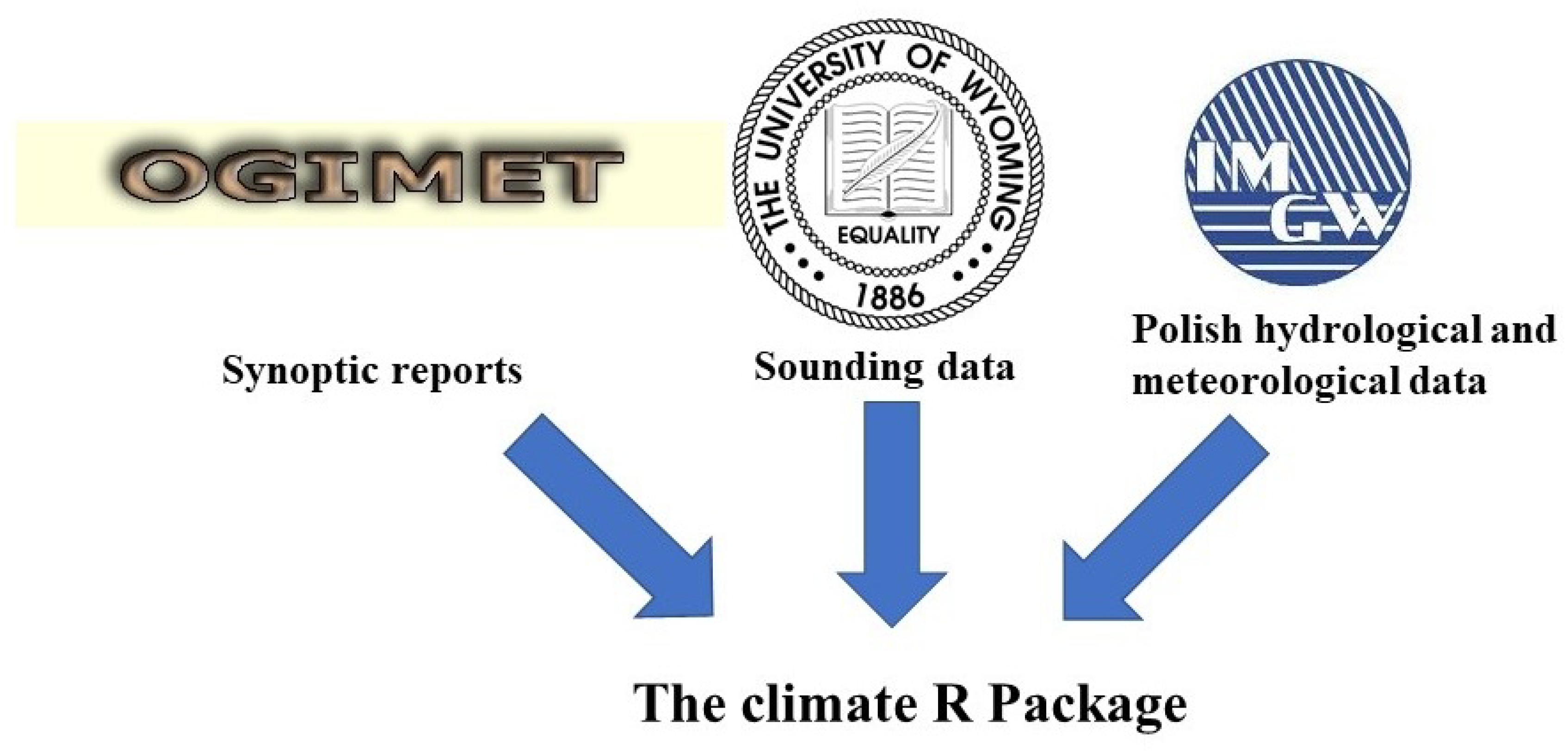
The availability of meteorological archive databases varies among countries. In most cases, access to such databases is usually not free of charge. However, the near-surface meteorological information from synoptic stations all around the world is publicly available free of charge due to the exchange of meteorological reports (e.g., FM-12 code established by the WMO) and is stored online. The ogimet.com web service is one of the most popular repositories of meteorological data that is heavily based on freely available data sources from the National Oceanic and Atmospheric Administration (NOAA) archives processed in a raw and human-readable format. Most of the archive dataset starts around the second part of 1999 and is being updated immediately after new reports are available.
The dataset representing atmospheric upper layers are also collected on the NOAA’s as well as an independent data repositories. In this study, a publicly available repository of the University of Wyoming (http://weather.uwyo.edu/upperair/sounding.html) was used, as it allows for downloading atmospheric data representing vertical profiles of the atmosphere on any of the global sounding stations dated back even up to 1960s. Moreover, this repository provides a quick summary of thermodynamic atmospheric indices, which also can be a useful source of information for interested groups of end-users.
Other data sources exist that can be more suited for locally targeted problems. Such an example is a data source provided by the Polish Institute of Meteorology and Water Management—National Research Institute (IMGW-PIB) that distributes their resources through an HTTP file server (https://dane.imgw.pl/). Thanks to the actions of the Polish atmospheric-related communities against limited access to collected data, the legislative changes were possible [13,14]. It ensured free access to meteorological and hydrological data for most commonly applied non-commercial use cases since January 2017. Nowadays, the way of the distribution of this operational data is one of the most liberal among European meteorological services.
A typical workflow of downloading meteorological data from a repository (e.g., Ogimet) conventionally using a web browser is to (1) select a country or station (2) for the given time range, and (3) measurement interval (i.e., hourly/daily). As a single query is limited to a few tens of rows per one search, thus creating a proper dataset requires manual and tedious routines. However, this approach is not a standard for all repositories. For example, the Polish hydro-meteorological repository requires a user to select the type of data, interval, and station of interest. Depending on the period and interval, a single (ZIP archive) file contains one- or five-years of observations with one or two files in every archive. Once the user selects the year (or five-year period), depending on the choices made earlier, they may encounter one set of files in the case of monthly synoptic data, three sets of files for the annual hydrological data, 13 sets for daily hydrological data, or about 60 sets in the case of hourly synoptic data. Each case has a separate data structure and different documentation. Overall, 23 possible cases for the meteorological and hydrological data exist, each requiring an individual approach for downloading and processing of the files. Since the beginning of 2017, the structure of these data has undergone numerous changes, which have confused some users, thereby discouraging them from using the repository.
The created package aims to supply access to the observational datasets which were missing so far among the R atmospheric community that had used mostly tools for downloading gridded or built-in datasets (e.g., ESD [15], rNOMADS [16], knmiR [17]). Partly this gap was covered by the rdwd package [18], however, its functionality is restricted to the products of the German Meteorological Service only. Keeping the aforementioned in mind, the main goal of the climate R package is to deliver a convenient way of accessing global and regional repositories containing meteorological and hydrological data. The choice of R [19] is related to the fact that this is currently one of the most popular programming languages among environmental researchers and data scientists, and simultaneously, it is free of charge. The created package aims at processing all formats of meteorological data independently of its origin in a tidy tabular form [20] that is suitable for various visualization and processing applications. Abbreviations of the variables are specified according to the WMO standards and were added to the package documentation. Relevant dictionaries attached to the climate package can be read by imgw_meteo_abbrev or imgw_hydro_abbrev commands. The created package also contains a database that clarifies the variables’ metadata and geographical coordinates of each stations’ location. Thanks to this feature, users can directly use the output data in geospatial analysis using R [21] programming language or external GIS software.

2. Methods and Materials

The climate package is distributed under the MIT license. However, users are obliged to follow the regulations provided on the respective webpages, as the package only provides an interface to the official repositories. The most stable version of the climate package is available at the Comprehensive R Archive Network (CRAN), while its developer version is hosted on the GitHub platform at http://rclimate.ml (mirrored to: https://github.com/bczernecki/climate), where third-party users can contribute to its further development.

2.1. Installation and User Guide

The climate package can be installed and run on any modern computer with the R environment version 3.1 or higher. The package was tested on a wide span of Windows instances and several Linux and Mac OS X distributions, and has positively undergone numerous tests before being published in the CRAN repository. The authors also deliberately avoided using external libraries in order to reduce possible dependencies or installation issues. The stable version of the climate package hosted on the official CRAN repository can be installed with the R’s install.packages("climate") and activated using the library(climate) commands respectively. The development version is hosted on the GitHub platform at (https://github.com/bczernecki/climate), where all instructions for installing and using the package are provided. Additionally, users are encouraged to contribute, leave feedback, or suggest their own ideas for further improvements that may be added in future releases.

2.2. Datasets

Archived data stored at (1) www.ogimet.com, (2) the University of Wyoming’s atmospheric sounding database and (3) in the official IMGW-PIB’s repository, constitute the primary sources for the data in the climate package (Figure 1).
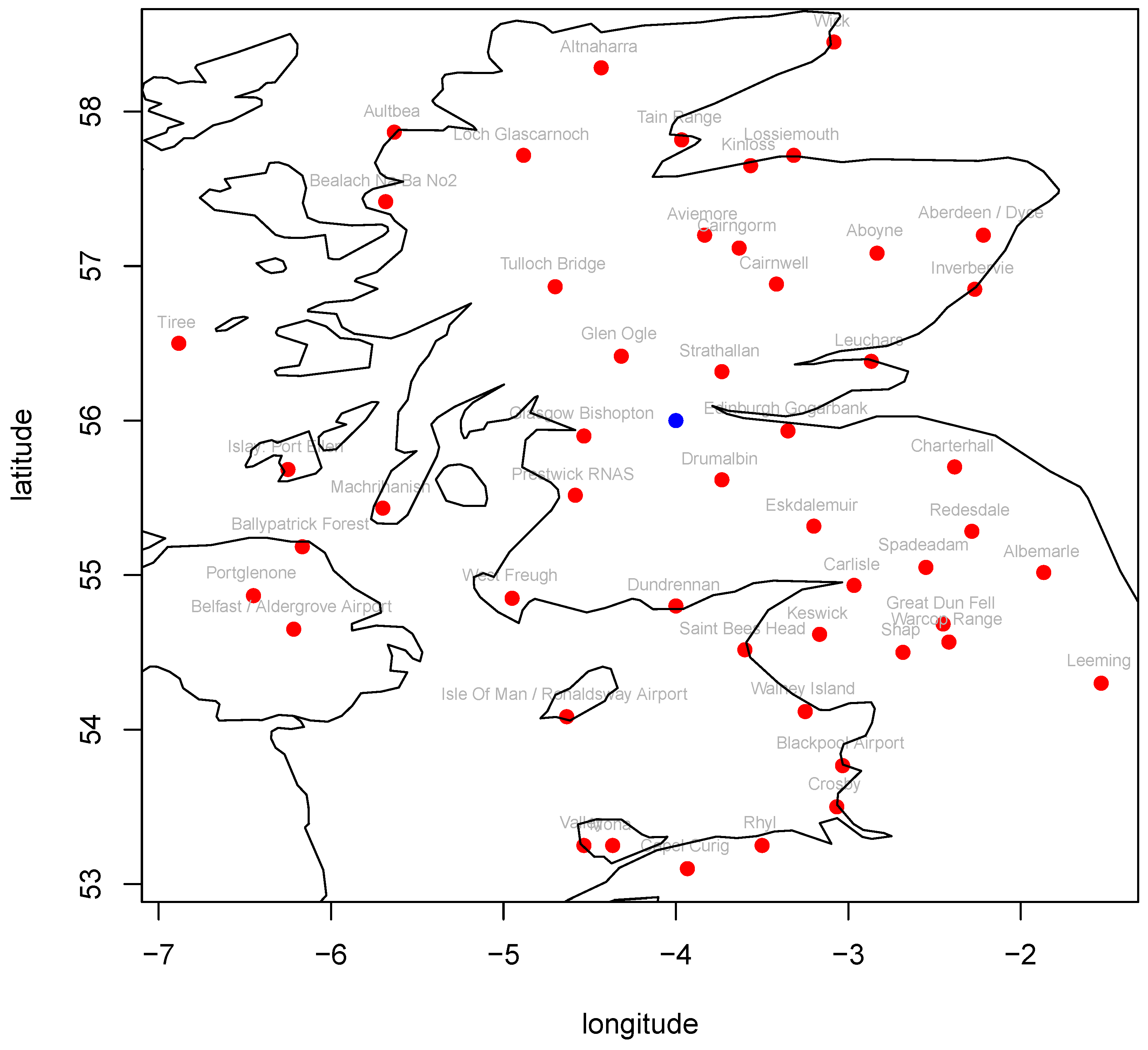
The synoptic reports available in the Ogimet web service are dated back to the year 1999. This global repository shares up to 17 variables (columns) representing instantaneous measurement for an individual station in a given date and time. Data is divided into daily and hourly time intervals. It contains information for the following: 2 meters air temperature (min., max., avg.) and dew point temperature [ ° C], atmospheric and sea level pressure [hPa], geographical coordinates [°], altitude [m], relative humidity [%], wind speed and wind gust [km · h 1 ], wind direction [direction], cloudiness [octants] and height of cloud base [km], visibility [km], sunshine duration and height of snow cover [cm].
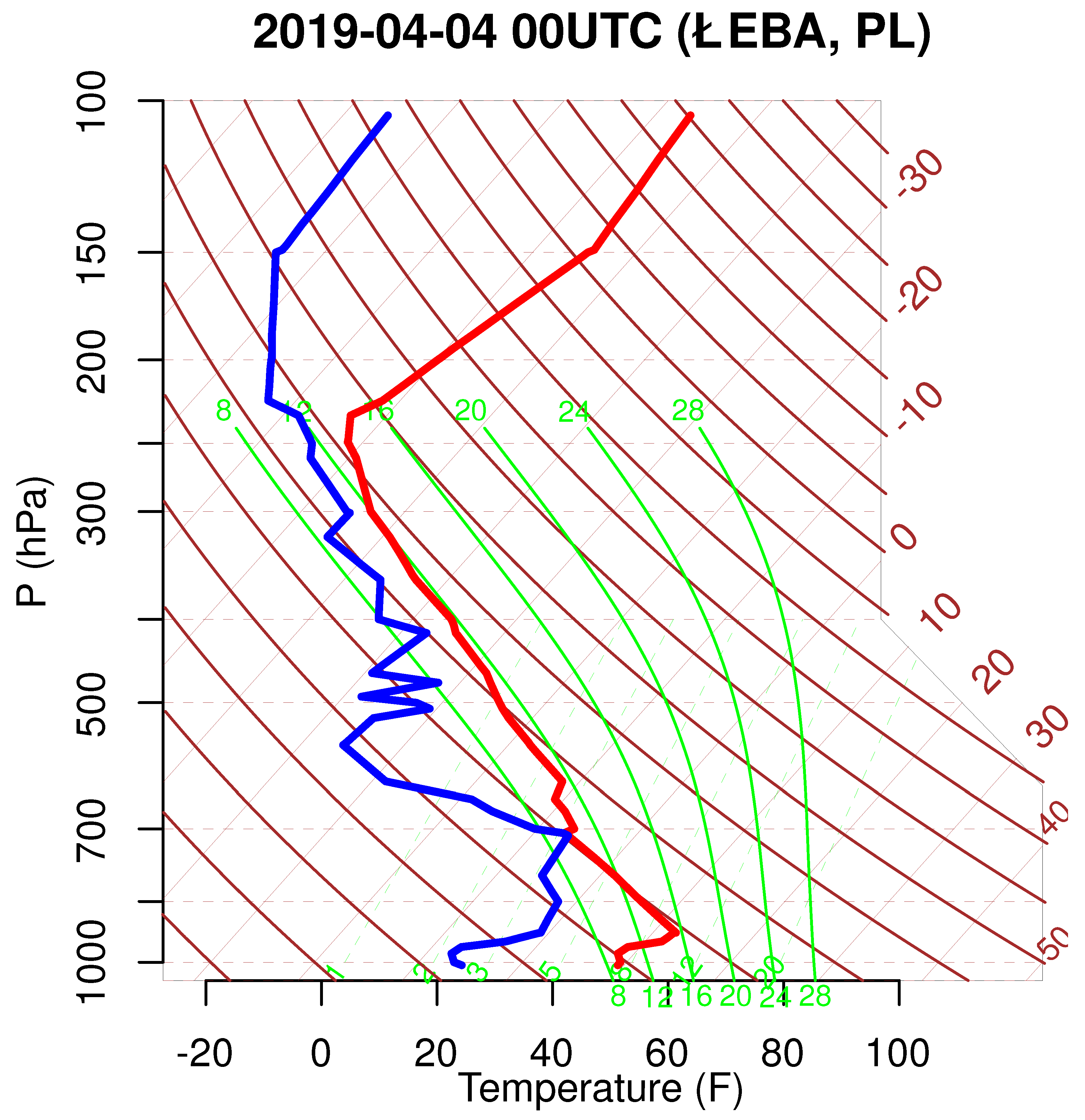
The historical sounding (i.e., upper air from the University of Wyoming’s repository) observations are not available on the Ogimet website. Therefore, this capability was added to the climate package due to the high demand for this kind of information among severe weather community, where it is commonly used for analyzing thermodynamic and kinematic atmospheric parameters [22,23]. This is also crucial information for identifying the atmospheric processes responsible for air quality problems [24]. The measurement interval is in most cases 12 hours (i.e., at 00 and 12 UTC, occasionally on some stations at 06 UTC and 18 UTC) and the data are usually available a few hours after beginning of the measurements. The sounding (also known as “rawinsonde”) data has 11 columns representing the instantaneous measurement of the atmospheric vertical profile for a single station and time. It contains information for the following parameters: atmospheric pressure [hPa], altitude [m], air temperature and dew point [ ° C], relative humidity [%] and mixing ratio [g · kg 1 ], wind speed [knots] and wind direction [°], and thermodynamic properties along with measurement metadata.
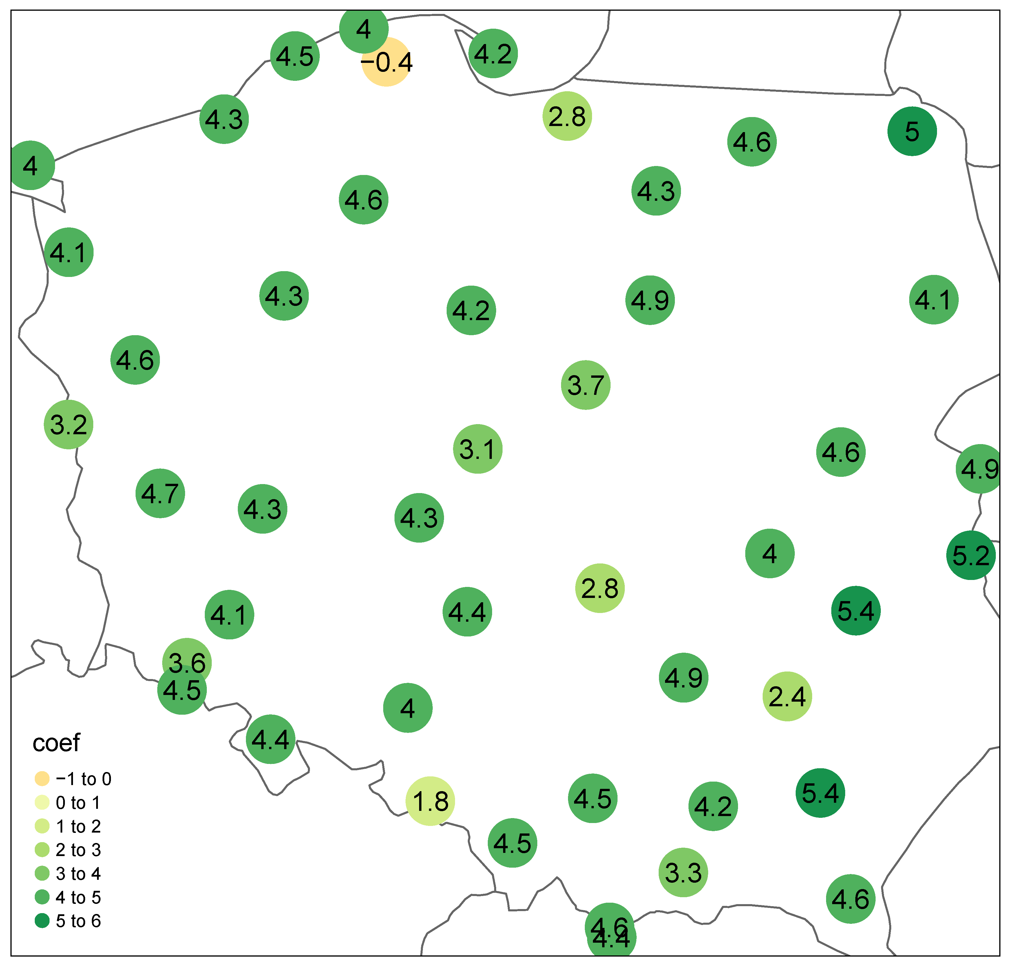
The IMGW-PIB (i.e., Polish hydro-meteorological) dataset contains measurements back to the 1950s, and the database is continually being updated, usually on a monthly basis. The meteorological data in the repository is divided, according to the hierarchy of stations, into (1) synoptic, (2) climatological, and (3) precipitation data. The synoptic and climatological stations consist of (1) hourly, (2) daily, and (3) monthly time intervals. The precipitation stations have no measurements at an hourly interval. The synoptic data are the most extensive and contain over 100 meteorological parameters. The climate data describes four essential meteorological components: air temperature [ ° C], wind speed [m · s - 1 ], relative humidity [%], and cloudiness [octants]. The precipitation data consist of the amount of precipitation with a description of the phenomena or surface precipitation type (i.e., rain, snow, snow cover height). Due to a relatively broad range of parameters obtainable for the meteorological data, the authors have thus decided to include a “vocabulary” that contains column names (i.e., meteorological parameters) in a (1) short, (2) more descriptive, or (3) original (Polish) forms. The hydrological data in the IMGW-PIB repository contains (1) daily, (2) monthly, and (3) semi-annual/annual measurements. All hydrological data uses the hydrological year, which begins on November 1st and ends on October 31st. Regardless of the temporal resolution, the hydrological data contains measurements of the maximum, mean, and minimum for the following: water flow [m 3 · s 1 ], water temperature [ ° C], and water level [cm]. Additionally, the daily dataset includes characteristics of the ice and overgrowth phenomena observed at the station. Similar to the meteorological dataset, a user can decide whether to add an extra description to the column names.

2.3. Core Functionality of the Climate R Package

The climate package currently consists of 21 functions with ten of them visible for the end-user (Table 1). Three of them are intended for downloading meteorological data, one for hydrological data, and four are auxiliary functions to improve the legibility and improve data exploration capabilities. Despite a relatively large number of functions that might be potentially used, there are four main functions called meteo_ogimet, sounding_wyoming, meteo_imgw and hydro_imgw that are generic wrappers for other functions. They allow for simplified downloading of any requested data in a convenient way. All available functions are documented on the package website and inside the built-in R help system where the exemplary code is also provided.

2.4. Ogimet Meteorological Data

The generic function for downloading decoded SYNOP reports from the Ogimet repository requires defining a set of arguments according to the schema provided below for the most generic meteo_ogimet function.
meteo_ogimet(interval, date, coords, station, precip_split)
where:
  • interval - temporal resolution of the data ("hourly", "daily") (argument not valid for: ogimet_hourly and ogimet_daily functions)
  • date - start and finish dates (e.g., date = c("2018-05-01", "2018-07-01") )—character or Date class object
  • coords—logical argument (TRUE or FALSE); if TRUE coordinates are added
  • station—WMO ID of meteorological station(s). Character or numeric vector
  • precip_split—whether to split precipitation fields into 6/12/24 h, numeric fields (logical value = TRUE (default) or FALSE); valid only for an hourly time step

2.5. Sounding Data

The proposed solution is based on the decoded TEMP sounding (radiosonde) reports hosted on the University of Wyoming (http://weather.uwyo.edu) server. It contains archived data for all upper air profiling stations working globally in the WMO network. The syntax for downloading the single sounding is as follows:
sounding_wyoming(wmo_id, yy, mm, dd, hh)
This function requires a few numeric arguments:
  • wmo_id—international WMO station code
  • year—year
  • mm—month
  • dd—day
  • hh—hour (usually radiosondes are launched at 00 and 12 UTC)
The returned object contains a list of two data frames. The first consists of measurements in a tabular form for 11 meteorological elements, while the second consists of metadata and the most fundamental thermodynamic and atmospheric instability indices.

2.6. IMGW-PIB Meteorological Data

The extended range of meteorological near-surface measurements can be achieved, usually from the regional met offices’ repositories. The publicly available Polish historical meteorological dataset comprises of two sections: meteorological and actinometrical data. Each of these sections is divided into subsections depending on the observational interval. The actinometric data was not implemented in the climate package due to ongoing changes to the data storage, and it will be added after the final format is determined.
The climate package contains an interface to the Polish IMGW-PIB dataset, which can be downloaded with a very similar syntax to the global dataset described previously in a simplified way. The schema shown below describes the use of the most generic meteo_imgw function and contains all arguments that can be used to define requested data.
meteo_imgw(interval, rank, year, status, coords, station, col_names)
where:
  • interval—temporal resolution of the data ("hourly", "daily", "monthly")
  • rank—type of the stations to be downloaded ("synop", "climate", or "precip")
  • year—vector of years (e.g., 1966:2000)
  • status—logical argument (TRUE or FALSE); for removing status of the measurements
  • coords—logical argument (TRUE or FALSE); if TRUE coordinates are added
  • station—vector of stations; it can be an ID of a station (numeric) or a name of a stations (capital letters)
  • col_names—three types of column names possible: “short”—default, values with shortened names, “full”—full English description, “Polish”—original names in the dataset
It is also worth noting that most of the arguments have predefined default values to support less experienced users. For example, if the station argument is not given, then all available datasets (here: data for all stations) are automatically downloaded. Only the interval, rank and year arguments are mandatory. In case any of them is not defined, the user is given a hint on the correct syntax.

2.7. IMGW-PIB Hydrological Data

The hydrological data is available in daily, monthly, and semiannual/annual temporal resolutions. The definition of the arguments in hydro_imgw is an analogue to the previously described for the meteorological data, with the syntax described below:
hydro_imgw(interval, year, coords, value, station, col_names)
where:
  • interval—temporal resolution of the data (“daily”, "monthly", "semiannual_and_annual")
  • year—vector of years (e.g., 1966:2000)
  • coords—logical argument TRUE or FALSE; if TRUE coordinates are added
  • value—type of data (can be: state—"H", flow—“Q”, or temperature—“T”).
  • station—vector of stations; it can be an ID of a station (numeric) or a name of a stations (capital letters)
  • col_names—three types of column names possible: “short”—default, values with shortened names, “full”—full English description, “polish”—original names in the dataset

3. Results

The purpose of this section is to show the capabilities of the created R package. The following subsections provide examples for types of analyses that can be performed using the climate R package together with other R packages available on CRAN.

3.1. Ogimet Meteorological Data—Use Case

The meteorological dataset use case provided below was based on hourly data from the Ogimet repository for the defined time frame, i.e., 2018/01/01 – 2018/12/31, for the location of Svalbard Lufthavn. The meteo_ogimet command allowed us to download 8761 observations for 22 variables (Listing 1). The dplyr and openair packages [25] were used to analyze and visualize part of downloaded results. After aggregating the data by the wind directions (the "ddd" column, Listing 2), converting directions into angles given in degrees, and reformatting dates’ classes, it was possible to align it to format required by external packages and plot the seasonal wind roses (Figure 2).
Listing 1. Example of the data download using the climate package.
library(climate)
df <- meteo_ogimet(interval = "hourly", date = c("2018-01-01", "2018-12-31"),
                   station = "01008")
#> [1]  "01008"
#> |======================================================================| 100 %
head(df[, 2:11])
#> DateTCTdCTmaxCTminCdddffkmhGustkmhP0hPaPseahPa
#>22018-12-3123:00:00−14.3−19.2<NA><NA>NNW25.243.21000.51004.2
#>32018-12-3122:00:00−13.7−18.2<NA><NA>NW21.632.41000.01003.8
#>42018-12-3121:00:00−15.9−18.5<NA><NA>ESE10.821.6999.91003.7
#>52018-12-3120:00:00−16.8−20.1<NA><NA>E18.025.21000.11003.9
#>62018-12-3119:00:00−17.2−21.7<NA><NA>ESE21.628.81000.51004.3
#>72018-12-3118:00:00−18.3−20.8−15.5−19.5ESE21.632.41000.71004.5
Listing 2. Example of a code used for creating a rose wind for Svalbard Lufthan in 2018.
library(climate)
# downloading data
df <- meteo_ogimet(interval = "hourly", date = c("2018-01-01", "2018-12-31"),
                   station = c("01008"))
library(openair) # external package for plotting wind roses
# converting wind direction from character into degrees
wdir <- data.frame(ddd = c("CAL", "N", "NNE", "NE", "ENE", "E", "ESE", "SE", "SSE",
                           "S", "SSW", "SW", "WSW", "W", "WNW", "NW", "NNW"),
                   dir = c(NA, 0:15  22.5), stringsAsFactors = FALSE)
# changing the date column to the format required by the openair package
df$date <- as.POSIXct(df$Date, tz = "UTC")
df <- merge(df, wdir, by= "ddd", all.x = TRUE) # joining two datasets
df$ws <- df$ffkmh/3.6 # converting to m/s from km/h
df$gust <- df$Gustkmh/3.6 # converting to m/s from km/h
windRose(mydata = df, ws = "ws", wd = "dir", type = "season", paddle = FALSE,
         main = "Svalbard Lufthavn (2018)", ws.int = 3, dig.lab = 3, layout = c(4, 1))

Searching for the Nearest Stations

The user can also use the climate package without knowing the station’s WMO ID. The nearest synoptic stations can be found with the nearest_ogimet_stations function (Listing 3). It requires users to provide a pair of geographical coordinates that point to the centroid of our area of investigations. We can specify how many nearest meteorological stations an user wants to find. As a result, we get a data frame with stations metadata and distance to given coordinates. Additionally a simple map can be added with the argument add_map = TRUE. Exemplary results and the code is given below Figure 3.
Listing 3. Example of downloading nearest stations according to a specified location (first six nearest stations are shown).
library(climate)
ns = nearest_stations_ogimet(country = "United+Kingdom", point = c(-4, 56),
               no_of_stations = 50, add_map = TRUE)
head(ns)
#> wmo_idstation_nameslonlataltdistance [km]
#>2903144Strathallan−3.73334856.316673546.44794
#>3203155Drumalbin−3.73334855.6166824552.38975
#>3003148Glen Ogle−4.31667356.4166756458.71862
#>2703134Glasgow Bishopton−4.53334455.900025960.88179
#>3503166Edinburgh Gogarbank−3.35000755.933355773.30942
#>2803136Prestwick RNAS−4.58334555.516682684.99537

3.2. Sounding Data—Use Case

Downloading data for a single vertical profile of the atmosphere requires providing date, hour, and station’s name (Listing 4). The chosen use case showed an atmospheric sounding started at 00UTC on 4th April 2019 in Łeba, Poland (Figure 4). The returned data frame from the measurements allowed users to plot temperature and humidity profiles on the Skew-T diagram generated thanks to the RadioSonde package [26]. It showed a strong thermal inversion up to 800–850 m a.g.l. which may strongly impact the air quality conditions in a near-surface layers [24]. The metadata and thermodynamic calculations stored in the second element of the returned list were omitted on purpose as no severe weather parameters related to atmospheric convection were detected.
Listing 4. Example of code to download sounding data, with Skew-T diagram.
library(climate)
library(RadioSonde) # an external package
profile <- sounding_wyoming(wmo_id = 12120,yy = 2019, mm = 4, dd = 4, hh = 0)
df <- profile[[1]]
colnames(df)[c(1, 3:4)] = c("press", "temp", "dewpt") # changing column names
RadioSonde::plotsonde(df, winds = FALSE, title = "2019-04-04 00UTC (LEBA, PL)",
                      col = c("red", "blue"), lwd = 3)

3.3. IMGW-PIB—Use Case

Another use case shows the possibilities of the climate package when coupled with the GIS and statistical capabilities of the R programming language (Figure 5). The downloaded data comprised 30 years of monthly mean air temperatures derived from the main meteorological stations in Poland. Due to the missing or suspicious diagnosed values, some data were excluded, e.g., stations’ location changes during the analyzed period or having a monthly mean air temperature during the summer season of 0 °C. The next step was to create a function for calculating the slope coefficient of the linear regression model that was later applied to the whole dataset.
The obtained results (Listing 5) were later transformed into a spatial object using the sf package [27] and visualized in the form of the map using the tmap package [28]. The created vector layer can later be saved in any GIS format supported by the sf package interfacing between R and the geospatial data abstraction library drivers (GDAL). One of the major advantages of using the R programming language is being able to keep everything in one environment instead of the typical situation where three different tools are applied for (1) data preprocessing, (2) statistical analysis, and (3) spatial data visualization. Such an approach makes it possible to reduce the required time for the entire research significantly and to focus more on the obtained results. However, the user must be aware that the provided tool is only an interface for downloading the data, and that the obtained results may inherit errors from the source repositories.
Listing 5. Exemplary code for downloading, processing and visualizing data from the IMGW-PIB repository.
library(ggplot2)
library(dplyr)
library(tidyr)
library(sf
library(tmap)
library(rnaturalearth)
library(climate)
ms <- meteo_imgw("monthly", "synop", year = 1978:2017, coords = TRUE)
# calculating annual values
ms %>%
  filter(!(mm > 5 && mm < 9 && t2m_mean_mon == 0)) %>%
  select(station, X, Y, yy, mm, t2m_mean_mon) %>%
  group_by(station, yy, X, Y) %>%
  summarise(annual_mean_t2m = mean(t2m_mean_mon), n = n()) %>%
  filter(n == 12) %>%
  spread(yy, annual_mean_t2m) %>%
  na.omit() -> trend
# extracting trends
regression <- function(x) {
  df <- data.frame(yy = 1978:2017, temp = as.numeric(x))
  coef(lm(temp ~ yy, data = df))[2]
}
trend$coef <- round(apply(trend[, -1:-4], 1, regression) * 100, 1)
trend <- st_as_sf(trend, coords = c("X", "Y"), crs = 4326)
# mapping the results
world <- ne_countries(scale = "medium", returnclass = "sf")
tm <- tm_shape(world) + tm_borders() +
  tm_shape(trend, is.master = TRUE) + tm_dots(col = "coef", size = 4) +
  tm_shape(trend) + tm_text(text = "coef")
tm

4. Conclusions

The climate R package allows users to obtain historical and most up-to-date meteorological information from both: ground and upper parts of the atmosphere. Data downloaded by climate gives possibilities for applying atmospheric data collected according to the WMO standards in an intuitive and fully automated way. The package is designed to be user-friendly and envisages, for the most part, environmental scientists wanting to obtain hydrological or meteorological data for research purposes in an convenient and programmable way within the R programming language. The usefulness and simplicity of the proposed solution can be especially valuable for many non-atmospheric scientists struggling with typically sophisticated and time-consuming mechanisms for accessing in-situ atmospheric data in a ready-to-use structure. The proposed solution with the climate package lets to save time for typical data flow in data science projects where a significant amount of time is spent on data preparation, while a core part of the computation is usually a magnitude shorter when compared to data cleaning and preprocessing [29].
Therefore for future improvements, it is planned to enlarge the climate R package with new local repositories so that more countries can conduct interdisciplinary research on meteorological data using a single tool, which can be targeted on a local scale in combination with global meteorological information. Also, new products (e.g., actinometric data in Poland) will be included once the IMGW-PIB repository has a mature form.

Author Contributions

Conceptualization, B.C., A.G. and J.N.; methodology, B.C., A.G. and J.N.; software, B.C., A.G. and J.N.; resources, B.C., A.G. and J.N.; writing–original draft preparation, B.C., A.G. and J.N.; visualization, B.C., A.G. and J.N. All authors have read and agreed to the published version of the manuscript.

Funding

This research was funded by the National Science Centre (NCN), Poland (Grants No.: UMO-2014/15/B/ST10/04455 & 2018/02/X/ST10/03113). The APC was funded by the Wrocław University of Environmental and Life Sciences.

Acknowledgments

The Institute of Meteorology and Water Management—National Research Institute as well as the University of Wyoming are the key sources of the data used in this paper. The authors would like to thank all volunteers and students of the Adam Mickiewicz University, Poznań who helped design the final structure of the package and have tested the developer version extensively since 2017.

Conflicts of Interest

The authors hereby declare no conflict of interest. All regulations and restrictions of data use can be found at: https://ogimet.com/, http://weather.uwyo.edu/upperair/sounding.html, and https://dane.imgw.pl/regulations, http://danepubliczne.imgw.pl.

Abbreviations

The following abbreviations are used in this manuscript:
CRANComprehensive R Archive Network
GDALGeospatial Data Abstraction Library
IMGW-PIBInstitute of Meteorology and Water Management—National Research Institute
METARMeteorological information used mostly by aircraft pilots
NOAANational Oceanic and Atmospheric Administration
SYNOPSurface synoptic observations
TEMPUpper air profiles
WMOWorld Meteorological Organization

References

  1. Schirmer, M.; Luster, J.; Linde, N.; Perona, P.; Mitchell, E.A.; Barry, D.A.; Hollender, J.; Cirpka, O.A.; Schneider, P.; Vogt, T.; et al. Morphological, hydrological, biogeochemical and ecological changes and challenges in river restoration—The Thur River case study. Hydrol. Earth Syst. Sci. 2014, 18, 2449–2462. [Google Scholar] [CrossRef] [Green Version]
  2. Szewrański, S.; Chruściński, J.; Kazak, J.; Świąder, M.; Tokarczyk-Dorociak, K.; Żmuda, R. Pluvial flood risk assessment tool (PFRA) for rainwater management and adaptation to climate change in newly urbanised areas. Water 2018, 10, 386. [Google Scholar] [CrossRef] [Green Version]
  3. Kendzierski, S.; Czernecki, B.; Kolendowicz, L.; Jaczewski, A. Air temperature forecasts’ accuracy of selected short-term and long-term numerical weather prediction models over Poland. Geofizika 2018, 35, 19–37. [Google Scholar] [CrossRef]
  4. Roshan, G.; Yousefi, R.; Błażejczyk, K. Assessment of the climatic potential for tourism in Iran through biometeorology clustering. Int. J. Biometeorol. 2018, 62, 525–542. [Google Scholar] [CrossRef] [PubMed]
  5. Bryś, K.; Brys, T. The First One Hundred Years (1791–1890) of the Wrocław Air Temperature Series. In The Polish Climate in the European Context: An Historical Overview; Springer: Berlin/Heidelberg, Germany, 2010; pp. 485–524. [Google Scholar]
  6. Głogowski, A.; Chalfen, M. Analysis of the effectiveness of the systems protecting against the impact of water damming in the river on the increase of groundwater level on the example of the Malczyce dam. In ITM Web of Conferences; EDP Sciences: London, UK, 2018; Volume 23, p. 00011. [Google Scholar]
  7. Grinn-Gofroń, A.; Nowosad, J.; Bosiacka, B.; Camacho, I.; Pashley, C.; Belmonte, J.; De Linares, C.; Ianovici, N.; Manzano, J.M.M.; Sadyś, M.; et al. Airborne Alternaria and Cladosporium fungal spores in Europe: Forecasting possibilities and relationships with meteorological parameters. Sci. Total Environ. 2019, 653, 938–946. [Google Scholar] [CrossRef] [PubMed]
  8. Czernecki, B.; Nowosad, J.; Jabłońska, K. Machine learning modeling of plant phenology based on coupling satellite and gridded meteorological dataset. Int. J. Biometeorol. 2018, 62, 1297–1309. [Google Scholar] [CrossRef] [PubMed] [Green Version]
  9. Frei, T. Economic and social benefits of meteorology and climatology in Switzerland. Meteorol. Appl. A J. Forecast. Pract. Appl. Train. Tech. Model. 2010, 17, 39–44. [Google Scholar] [CrossRef]
  10. Palmer, T.N. The economic value of ensemble forecasts as a tool for risk assessment: From days to decades. Q. J. R. Meteorol. Soc. A J. Atmos. Sci. Appl. Meteorol. Phys. Oceanogr. 2002, 128, 747–774. [Google Scholar] [CrossRef]
  11. Kalnay, E.; Kanamitsu, M.; Kistler, R.; Collins, W.; Deaven, D.; Gandin, L.; Iredell, M.; Saha, S.; White, G.; Woollen, J.; et al. The NCEP/NCAR 40-year reanalysis project. Bull. Am. Meteorol. Soc. 1996, 77, 437–472. [Google Scholar] [CrossRef] [Green Version]
  12. Miętus, M. O przydatności rezultatów globalnych reanaliz NCEP i ERA-40 do opisu warunków termicznych w Polsce; Instytut Meteorologii i Gospodarki Wodnej: Warsaw, Poland, 2009. [Google Scholar]
  13. Council of Poland. Law of 25.02.2016. about Re-Use of Public Sector Information (Dz. U. z 2016 r., pos. 352., with Later Changes). 2016. Available online: http://prawo.sejm.gov.pl/isap.nsf/DocDetails.xsp?id=WDU20160000352 (accessed on 1 December 2019).
  14. Council of Poland. Law of 20.07.2017 the Water Act (Dz. U. z 2017 r. pos. 1566). 2017. Available online: http://prawo.sejm.gov.pl/isap.nsf/DocDetails.xsp?id=WDU20170001566 (accessed on 1 December 2019).
  15. Benestad, R.E.; Mezghani, A.; Parding, K.M. ‘esd’-The Empirical-Statistical Downscaling tool & its visualisation capabilities; Met Report 11/15; Norwegian Meteorological Institute: Oslo, Norway, 2015. [Google Scholar]
  16. Bowman, D.C.; Lees, J.M. Near real time weather and ocean model data access with rNOMADS. Comput. Geosci. 2015, 78, 88–95. [Google Scholar] [CrossRef]
  17. Buishand, T.A.; De Martino, G.; Spreeuw, J.; Brandsma, T. Homogeneity of precipitation series in the Netherlands and their trends in the past century. Int. J. Climatol. 2013, 33, 815–833. [Google Scholar] [CrossRef] [Green Version]
  18. Boessenkool, B. rdwd: Select and Download Climate Data from ‘DWD’ (German Weather Service), R package version 1.2.0; Deutscher Wetterdienst: Offenbach, Germany, 2019. [Google Scholar]
  19. R Core Team. R: A Language and Environment for Statistical Computing; R Foundation for Statistical Computing: Vienna, Austria, 2013. [Google Scholar]
  20. Wickham, H. Tidy data. J. Stat. Softw. 2014, 59, 1–23. [Google Scholar] [CrossRef] [Green Version]
  21. Lovelace, R.; Nowosad, J.; Muenchow, J. Geocomputation with R; CRC Press: Boca Raton, FL, USA, 2019. [Google Scholar]
  22. Blumberg, W.G.; Halbert, K.T.; Supinie, T.A.; Marsh, P.T.; Thompson, R.L.; Hart, J.A. SHARPpy: An open-source sounding analysis toolkit for the atmospheric sciences. Bull. Am. Meteorol. Soc. 2017, 98, 1625–1636. [Google Scholar] [CrossRef]
  23. Taszarek, M.; Brooks, H.E.; Czernecki, B. Sounding-derived parameters associated with convective hazards in Europe. Mon. Weather Rev. 2017, 145, 1511–1528. [Google Scholar] [CrossRef]
  24. Nidzgorska-Lencewicz, J.; Czarnecka, M. Winter weather conditions vs. air quality in Tricity, Poland. Theor. Appl. Climatol. 2015, 119, 611–627. [Google Scholar] [CrossRef] [Green Version]
  25. Carslaw, D.C.; Ropkins, K. Openair—An R package for air quality data analysis. Environ. Model. Softw. 2012, 27, 52–61. [Google Scholar] [CrossRef]
  26. Nychka, D.; Gilleland, E.; Zhang, L.; Hoar, T. RadioSonde: Tools for Plotting Skew-T Diagrams and Wind Profiles, R package version 1.4; University Corporation for Atmospheric Research: Boulder, CO, USA, 2014. [Google Scholar]
  27. Pebesma, E. Simple features for R: Standardized support for spatial vector data. R J. 2018, 10, 439–446. [Google Scholar] [CrossRef] [Green Version]
  28. Tennekes, M. tmap: Thematic Maps in R. J. Stat. Softw. 2018, 84, 1–39. [Google Scholar] [CrossRef] [Green Version]
  29. Wickham, H.; Grolemund, G. R for Data Science: Import, Tidy, Transform, Visualize, and Model Data; O’Reilly Media, Inc.: Sebastopol, CA, USA, 2016. [Google Scholar]
Figure 1. The data sources used in the climate R package.
Sustainability 12 00394 g001
Figure 2. Seasonal wind roses for Svalbard Lufthavn in 2018 based on Ogimet dataset.
Sustainability 12 00394 g002
Figure 3. Example code for searching for the 50 nearest stations from the point of given coordinates (longitude 5° W, latitude 56° N) in United Kingdom. First 22 records are shown in Listing 3.
Sustainability 12 00394 g003
Figure 4. Example of a downloaded sounding dataset plotted on Skew-T diagram.
Sustainability 12 00394 g004
Figure 5. Air temperature trends in Poland per 100 years ( ° C) based on the calculated slope of linear regression for 1978-2017—IMGW-PIB dataset.
Sustainability 12 00394 g005
Table 1. The essential user-visible functions available in the climate package.
FunctionDescription
Meteorological data—download
meteo_ogimetA generic function for downloading hourly and daily dataset from the Ogimet repository
sounding_wyomingA function for downloading sounding (i.e., upper air) data for any station in the world (i.e., vertical profiles of the atmosphere) from the University of Wyoming repository
meteo_imgwA generic function for downloading hourly, daily and monthly meteorological dataset from the IMGW-PIB repository
Hydrological data—download
hydro_imgwA generic function for downloading daily, monthly, and annual hydrological dataset from the IMGW-PIB repository
Auxiliary functions and datasets
stations_ogimetA function for downloading information about all stations available for the selected country in the Ogimet repository
nearest_stations_ogimetA function for downloading information about nearest stations to the selected point available for the selected country in the Ogimet repository
imgw_meteo_stationsBuilt-in metadata for meteorological stations, their geographical coordinates, and ID numbers (from the IMGW-PIB repository)
imgw_hydro_stationsBuilt-in metadata for hydrological stations, their geographical coordinates, and ID numbers (from the IMGW-PIB repository)
imgw_meteo_abbrevDictionary explaining variables available for meteorological stations (from the IMGW-PIB repository)
imgw_hydro_abbrevDictionary explaining variables available for hydrological stations (from the IMGW-PIB repository)

