2.1. General Description of the Analytical Model
Consider a generic service region containing a hieratical transit network composed of two transit modes: the flexible on-demand transport service and the urban railway transit. The DRT serves as the feeder that collects passengers based on real-time requests and delivers them to railway stations. This operation mode is similar to the operating strategy for “many-to-one” systems [
8], in which a fleet of homogeneous vehicles is assumed to travel in cycles, collecting passengers from their origins to railway stations. With perfect information (including the schedule information of both DRT and railway services), which can be easily obtained from the transit information platform provided by the agency (e.g., websites, smartphone applications), passengers are assumed to be able to decide their pick-up times aimed at catching the rail transit on time.
The service region is assumed to be characterized by its area, the number of railway stations, the spatial density of passengers over the region, and the depot location. Suppose a service region
A with area
A. Let
denote the set of indices for railway stations in the service region and
be a particular station. We assume that each transit station serves a subregion of
, which is known as the “catchment area” [
29] that encompasses an area of potential passengers that would be willing to access this station. Each subregion is approximated by a rectangle with length and width, served by a fleet of homogeneous vehicles. Let
denote the subregion served by station
with area
. For simplicity, the service region is defined as fully covered by the subregion, that is,
. The user demand within the area is assumed to be spatially uniformly distributed within a given time interval of the day with a spatial density
(number of users per unit area). Considering the full flexibility of the DRT service, stops of the DRT vehicle are according to the real-time passenger requests. The total number of stops,
, in area
is equal to the number of passengers, that is,
.
A fleet of identical vehicles with capacity
(pax) is assumed to be allocated by the agency in the service area. Passengers make trip requests through the information platform to the agency to specify their desired pickup location and time. A nearest-neighbor routing strategy is adopted where each bus always picks up the nearest passenger who is waiting in the system. In the remainder of this section, a continuum approximation is firstly adopted to analyze the agency cost. Then, considering the queueing phenomenon, the Vickrey [
11] queueing theory is adopted as the basis for approximating each component of the user cost.
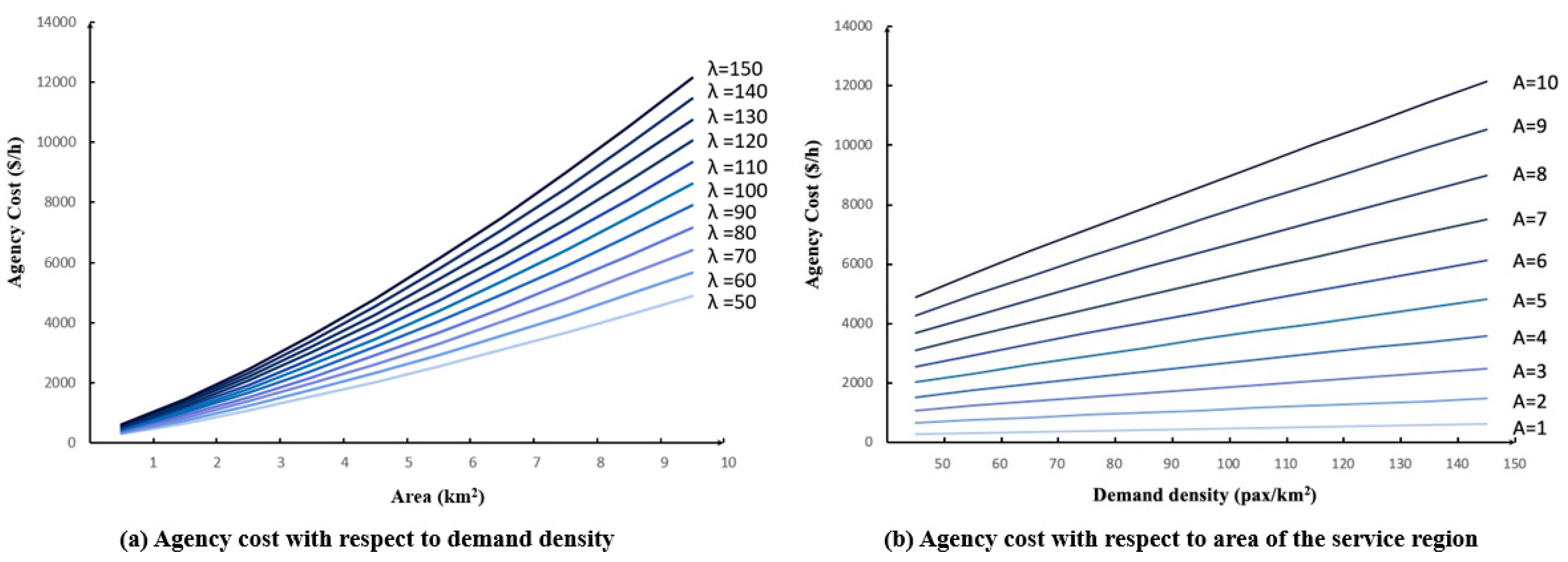
2.2. Agency Cost
The agency costs in the DRT system include the expected total distance that vehicles travel in the network and the expected total fleet size needed in operation. The DRT network is constructed by a number of bus trips, each of which serves a railway station. More specifically, a bus trip begins at the depot and then travels to a subregion of size
to visit passengers in this area via a Hamiltonian path [
30], while the number of passengers is obtained by
. In this study, it is assumed that the depot is located outside the service area
. Hence, it is common to decompose the expected distance of a DRT trip for a certain station, denoted as
, into three components: (i) the expected distance from the origin of the trip (e.g., the depot) to the first user in the subregion
,
; (ii) the expected distance from the first user to the last user within
,
; and (iii) the expected distance form the last user on the trip to the rail station,
. Hence,
In continuum approximation analysis, the routing details within the vehicle service area are usually modeled approximately in terms of continuous variables, i.e., the spatial density [
8]. Analytical models were developed in previous studies [
26,
31], which aimed at investigating the relationship between the tour length and the average number of passengers in service areas of different shapes based on the formulation in References [
24,
25]. For a spatially uniformly distribution of passenger demand,
can be estimated by the expected distance from the depot to a passenger in
which is randomly located. Suppose that the distance from the origin of the trip (e.g., the depot) to the centroid of
is
. As developed by Campbell [
31],
can be calculated by the product of a factor,
, which is related to
, and the square root of
, that is,
.
indicates the sum of vehicle “peddling” distance with respect to the number of passengers in
, which highly depends on the routing strategy the agency applied based on the specific circumstances of the serving area, such as demand density. Let
denote the distance from the centroid of
to station
.
can then be obtained by
.
In previous studies, the nearest-neighbor approach was widely adopted to approximate the expected passenger-to-passenger distance, in the analytical model of many-to-one or many-to-many dial-a-bus systems with respect to the passenger demand density [
2,
7,
17,
21]. It was proven to be a reasonable approximation and an efficient routing strategy. More specifically, after each pick-up service, the demand-responsive vehicle is routed to the nearest passenger who made the request. The approximation of the average distance to the nearest
uniformly distributed passengers over
can be written as
where
is the “peddling factor” defined by Daganzo [
25] and Campbell [
31], which is given in
Table 1.
In sum, the total expected distance of a DRT trip for station
j can be written as
Note that Daganzo [
24] and Campbell [
31] illustrated that the value of
is related to three factors: (i) the distance metric (Euclidean or Manhattan), (ii) the distance between the origin/destination and the service area
, and (iii) the shape of
. In this paper, it is assumed that all distances are given by the Euclidean metric.
can be determined from the equation developed by Vaughan [
32].
Additionally, the agency should hold a sufficient number of vehicles to serve all passengers. Daganzo [
21] illustrated that the minimum fleet size needed to satisfy the demand in an area depends on the average time that each passenger spends in the vehicle, which is composed of the stop time (e.g., pick-ups and drop-offs) and in-vehicle riding time. In the collection phase, the extra time required to serve an additional passenger includes the pick-up and drop-off times, as well as the vehicle riding time for the pick-up of the passenger. Hence, for a certain vehicle
i, the length of the collection phase can be expressed as
where
is the sum of pick-up and drop-off times,
is the average vehicle speed, and
is the average distance traveled by the vehicle from a passenger to the next one when there are
passengers in the service area.
is the number of passengers collected by vehicle
. The total service rate can be obtained by the sum of individual vehicles’ service rates deployed in an area.
where
is the fleet size that the agency can use to adequately serve the demand by providing the total system service rate
in this area. It is obvious that the vehicle collection time is an increasing function of the number of passengers waiting to be picked up. The attempt of collecting more passengers would inevitably result in a longer collection time, as well as an elongated average in-vehicle riding time for passengers on board, which has a negative effect on the system’s level of service. Hence, one important design trade-off is between the level of service and the number of passengers each vehicle collects. Several studies illustrated that the best level of service is achieved when the number of passengers in each vehicle is equal [
17,
21]. Hence, Equation (6) can be rewritten as
In the meantime, the optimal fleet size required in a certain area (say subregion ) can be obtained by , where is the number of passengers for each vehicle collected in subregion .
To sum up, the total operating distance of the agent can be represented as
where
is the required fleet size in subregion
.
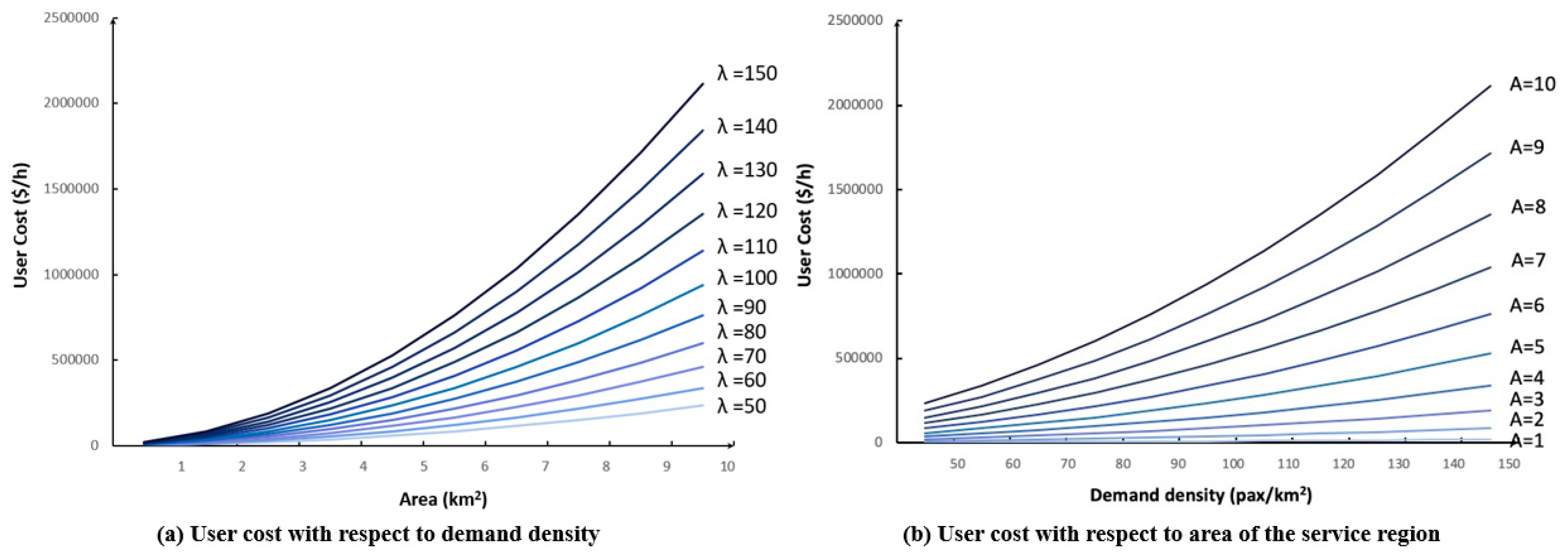
2.3. User Cost
In the DRT system, the agency provides a flexible door-to-door transportation service based on real-time users’ requests. Experienced users who are assumed to have the full information of the system may evaluate their general costs including queueing delay and schedule deviations relative to their desired pick-up times, and they may maintain their trips by choosing their own requested pick-up times. Additionally, aimed at improving the operation efficiency, the agency prefers to elongate the route and deviate to collect more passengers. An unavoidable inconvenience would, however, be incurred for the passenger through the increased in-vehicle riding time [
33]. Except for the queueing delay and schedule deviations, it is reasonable to consider the in-vehicle riding time as an irreducible component of the user cost.
Consider that, in a generic subregion
, the passengers are scattered throughout and wish to be picked up at the moment of their requests. Once the service rate is determined by the agency, it is broadcasted to all passengers to determine when they would make a request. Although making a request as early as possible might be a rational decision, the early boarding may cause other costs, e.g., the in-vehicle waiting time for the last passenger to board the vehicle. Each individual would wisely determine the request time to balance each component of their travel cost, including the waiting time in the queue out of the vehicle, the earliness penalty, the lateness penalty, and the waiting time for the departure of the vehicle. Thus, the total travel cost for a passenger arriving at time
t is
where
(
$/time) is the cost rate that each passenger values in terms of the time in queues occurred out of the vehicle and in the vehicle. The cost rates of earliness time and lateness time are
and
, respectively, where scalars
and
satisfy
[
34,
35]. The cost rate of in-vehicle waiting delay is represented by
. Furthermore, all passengers are assumed to be well-informed and rational, all of whom have an identical perception of each component of their costs.
The DRT system is assumed to be operated on a first-in-first-out order basis. In other words, no one can be picked up earlier upon making a request later. In an oversaturated system, the passenger demand rate will exceed the service rate because of the adequate operating capacity, which makes it impossible for vehicles to serve all passengers at the time they make requests. Rational passengers could adapt their request times by putting forward or postponing their requests to minimize their own travel costs. The passenger who boards the vehicle earlier has to stay in the vehicle, while the vehicle detours to pick up other passengers who requested the pick-up service. The cumulative result of these individual decisions would also lead to an equilibrium condition where no one has an incentive to change their request times. Considering these similarities, the passengers’ request time choice behavior can be described by the Vickrey’s equilibrium model [
7,
11,
35]. The trade-offs of the passenger’s travel cost lie in the tolerance of increased delay in waiting for pickups or longer in-vehicle time, as well as schedule deviations, which also depend on the service quality of the DRT system. In practice, the service quality or the performance of the DRT system is directly or indirectly influenced by many factors, especially the routing strategy adopted by the operator [
7].
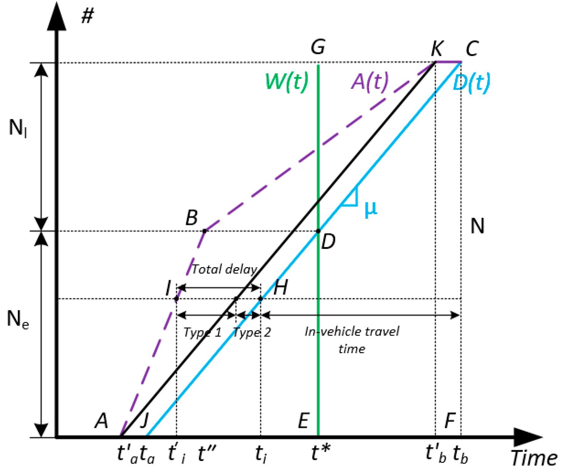
Figure 1 illustrates the cumulative result of passengers using the DRT system in the equilibrium condition. Let
denote the first passenger’s request time and
denote the last passenger’s request time, which also are the starting and ending times of the queue in the DRT system of subregion
.
depicts the cumulative distribution of passengers’ wished pick-up time. In this study, the passengers are assumed to have a common boarding time
, which is also illustrated by line
.
is the cumulative pick-up curve, which describes the times when the passengers are actually picked up by the vehicle. The performance or the quality of service of the queueing system can be measured by the slope of
, which is defined as the service rate (or effective system capacity, which indicates the number of passengers serviced per unit time) in
Section 2.2 (see Equation (7)).
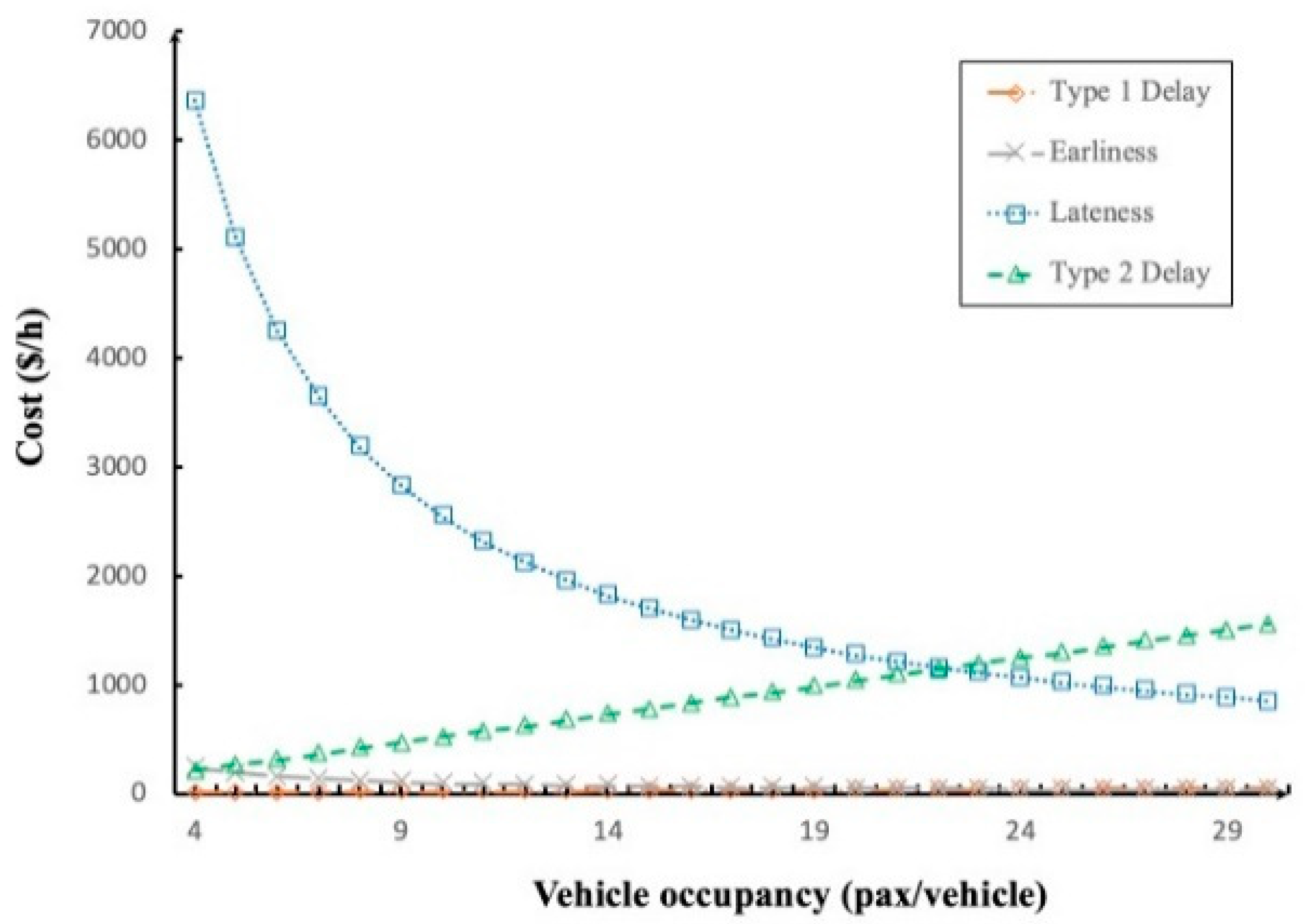
In the case where the vehicle detours over the region, the visiting sequence of passengers is scheduled as they enter the system, which can be seen as a queue that forms virtually in the DRT system. Suppose that a generic passenger is considered as the next one to be served, an extra waiting time is incurred because the vehicle has to travel from its current position to this passenger. In other words, two types of delay can be found: virtual queueing delay (termed as Type 1 delay) and actual vehicle traveling delay (termed as Type 2 delay). As illustrated in
Figure 1, the first passenger who makes a request at
would experience no virtual queueing delay but an unavoidable delay that indicates the minimum travel time required for the vehicle to receive the request and pick up the first passenger. Considering that the passengers are uniformly distributed within the subregion, this temporal gap,
, can be approximated by the average passenger-to-passenger travel distance divided by the vehicle speed, that is,
. Similarly, the last passenger has Type 2 delay only because they make the request at the time when there are no other passengers waiting in the system.
In the remainder of this section, we focus on the derivation of the UE passenger queueing pattern based on the bottleneck in an oversaturated DRT system in the subregion j. For notation simplicity, we consider the subregion j as a generic service region and omit the subscript j in all relevant notations.
Following Wardrop’s first principle [
36], it is assumed that, at equilibrium, passengers are subjected to the same total travel cost regardless of their request time for the service. Hence, the sum of schedule deviation and in-vehicle waiting costs for the first request is equal to the schedule delay cost of the last.
where the term of
is subtracted from both sides of the above equation. Since all passengers are picked up during the time period (
ta,
tb), we have the following equation:
where
is the total number of passengers in the service region. Simultaneously solving Equations (10) and (11), we can obtain the starting and ending times of the queue.
As shown in
Figure 1, assume that the passenger who is picked up by the vehicle at time
(Point
), makes a request at time
, which means that the waiting time in the queue is
. The passenger who is picked up punctually at his wished pick-up time at time
bears the longest waiting time of
. Recalling the UE principles that passengers have the same costs, this yields
The solution of Equation (14) is shown as follows:
It is obvious that the cumulative of the request curve to the pick-up service,
, is a piecewise linear curve (cumulative curve from point
to
) (see
Figure 1). The remainder of this section provides the proof of this proposition.
Consider that an early passenger who is the
n-th passenger makes a request before
. The total travel cost of the
n-th passenger is
where
and
are the inverse functions of
and
, which denote the starting and ending queuing times of the
-th passenger, respectively. The equilibrium condition is obtained when no one has the incentive to change their arrival time at the queue as follows [
37,
38,
39]:
According to the property of the inverse function,
By integrating Equations (18)–(20), we obtain
It is obvious that both
and
are linear functions. The slop of
is
Correspondingly, the slop of
during
is given by
In contrast to previous papers where the total travel cost in the Vickery’s equilibrium model was composed of queueing delay and schedule deviations only [
7,
11,
36,
39,
40], the additional consideration of the in-vehicle delay cost in this paper would also result in two new equilibrium conditions. Firstly, the proportion of the early passengers,
, to the late passengers,
Nl, is equal to
and
. Secondly, the request curve in equilibrium is piecewise linear and must satisfy
In the equilibrium condition, no one can reduce their travel time by making the request earlier or later. As a result, the critical passenger who is picked up at the time they wish would suffer the maximum delay (making request at point
B).
On the basis of the passenger queueing model in the DRT system, the approximation of user cost is presented in the remainder of this section. The passenger’s total queueing delay (including both types of delay) is defined as the time difference between the time that the passenger makes a request and the time they are considered as the next one to be served, i.e., the horizontal distance between
A(
t) and
in
Figure 1. It is obvious that these two types of delay can be calculated separately. The Type 1 delay can be approximated by the area between
and line
AK, which depicts the cumulative distribution of times that passengers are taken as the next ones to pick up. Additionally, passengers are assumed to experience the same Type 2 delay in that passengers are uniformly distributed in the service area. Accordingly, the total delay that all passengers experience waiting to be picked up can be approximated by the area between
and
in
Figure 1.
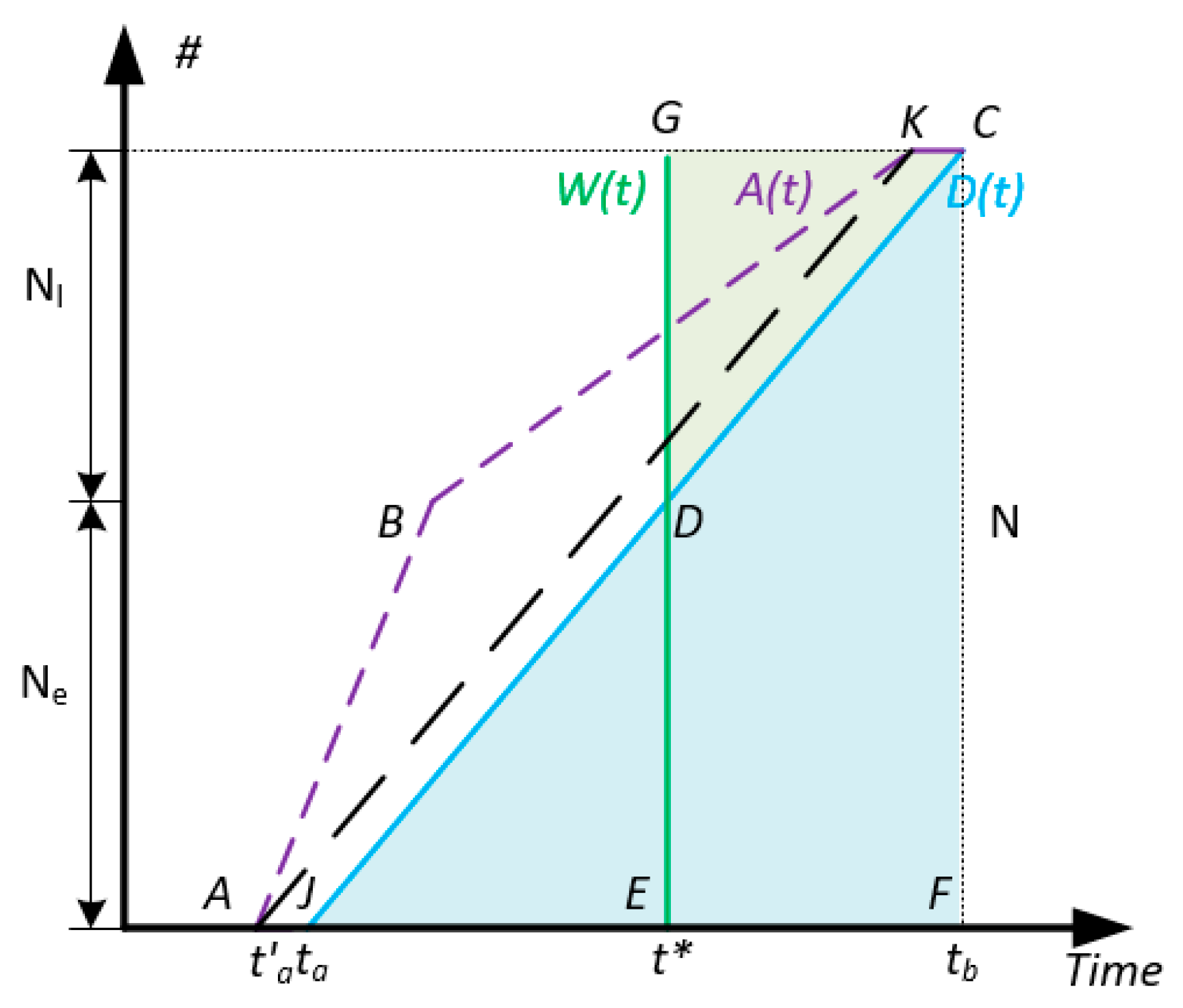
Earliness and lateness are defined as the temporal difference between the actual and wished boarding times. Hence, as shown in
Figure 2, the total earliness for all passengers can be approximated by the area between
D(
t) and the wished curve
from
to
(triangle
), while the total lateness is approximated by the area between
and
from
to
(triangle
). The approximations of total earliness and lateness are presented as follows:
By definition, the in-vehicle riding time for an individual passenger is measured by the difference between the time they are actually picked up and the ending time of the collection. As depicted in
Figure 1, the total in-vehicle riding cost is proportional to the area of triangle
CFJ, which can be approximated as follows:
In sum, the total travel cost of the passenger is confirmed to be the summation of the total waiting costs, including both out-of-vehicle and in-vehicle costs, and the total schedule deviations,


