A Residential Load Scheduling with the Integration of On-Site PV and Energy Storage Systems in Micro-Grid

Abstract

The smart grid (SG) has emerged as a key enabling technology facilitating the integration of variable energy resources with the objective of load management and reduced carbon-dioxide (CO${}_2$) emissions. However, dynamic load consumption trends and inherent intermittent nature of renewable generations may cause uncertainty in active resource management. Eventually, these uncertainties pose serious challenges to the energy management system. To address these challenges, this work establishes an efficient load scheduling scheme by jointly considering an on-site photo-voltaic (PV) system and an energy storage system (ESS). An optimum PV-site matching technique was used to optimally select the highest capacity and lowest cost PV module. Furthermore, the best-fit of PV array in regard with load is anticipated using least square method (LSM). Initially, the mathematical models of PV energy generation, consumption and ESS are presented along with load categorization through Zero and Finite shift methods. Then, the final problem is formulated as a multiobjective optimization problem which is solved by using the proposed Dijkstra algorithm (DA). The proposed algorithm quantifies day-ahead electricity market consumption cost, used energy mixes, curtailed load, and grid imbalances. However, to further analyse and compare the performance of proposed model, the results of the proposed algorithm are compared with the genetic algorithm (GA), binary particle swarm optimization (BPSO), and optimal pattern recognition algorithm (OPRA), respectively. Simulation results show that DA achieved 51.72% cost reduction when grid and renewable sources are used. Similarly, DA outperforms other algorithms in terms of maximum peak to average ratio (PAR) reduction, which is 10.22%.

1. Introduction and Motivation

With the rapid increase in population and economic growth, global energy consumption is also increasing drastically. High reliance on fossil fuel and increased use of thermal power resources contributed to an increase in CO${}_2$ emissions that causes an increase in global warming [1]. While adopting the ways to tackle the increased energy demand, a reduction in greenhouse gas emissions is a major challenge that must be met on a global scale in order to promote energy sustainability. In recent years, while reducing the gap between energy generation and demand through a combination of thermal and nuclear energy resources, the pursuit of power generation through renewable energy sources, such as solar, wind, biomass and lowering environmental load, has been promoted with the aim of reducing greenhouse gas emissions, significantly. Renewable energy is becoming widely accepted as a new source of energy to provide power to residential and commercial buildings around the world. On the other hand, energy is one of the basic necessities for sustainable development of society that must surely be delivered in an efficient way in order to promote a green environment with reduced CO${}_2$ emissions [1]. However, the great paradigm shift due to the involvement of information and communication technologies (ICTs) the traditional ways of energy generation, transmission and distribution need to be upgraded [2,3,4,5,6,7,8]. The author in [9] presented a hybrid opinion network containing of continuous and discrete valued agents. This model discussed a communication behavior for social dynamical systems. The scaled consensus of switching topologies with continuous and discrete time subsystems is investigated. The traditional electricity infrastructure is not fully capable of handling and managing the distributed energy resources with high quality of communication service and grid stability. This is due to the fact that increasing energy demand needs extra costlier generation or back-up reserve capacity units that lead to high tariff rates and CO${}_2$ emissions.

Therefore, to cope with such types of situations, a smart grid (SG) concept has recently been introduced which has the capability to fulfil the load demand that benefices both the end users and utility market [10]. The users can enjoy an uninterruptible power supply with economical tariff rate and utility can avail the opportunity to improve power system stability through supply–demand balance. The former can be achieved by exploiting efficient load management through distributed as well centralized control strategies [11]. For this purpose, different researchers introduced residential and commercial load scheduling techniques considering both end user and utility objectives [12,13]. Among these solutions, the major emphasis is given to balance the load demand through market supply without heavily relying on peak power plants and reserved capacity units [14]. However, some researchers focussed on balancing the load demand through load scheduling and energy management using optimization technique. Although these kinds of techniques are efficient in managing the load demand with partial or full control on residential load [15]. The peaks and troughs in the aggregated user energy demand profile are caused by the temporal variations in energy demand. The user’s participation is required in balancing the load by allowing the grid to reschedule the load. However, the end users are affected due to unplanned load scheduling by the grid [16]. For example, it is assumed that the user suffers the same degree of inconvenience if base and/or non-flexible load is shifted in either direction (before or after) of its most preferred time slot. In other words, delaying a base and/or non-flexible load by 2 time slots or advance scheduling the same load by 2 time slots will result in same amount of user inconvenience. To handle this situation, some researchers put their efforts into devising the load control strategies with major focus on load scheduling without disturbing end users’ objectives [17]. Furthermore, it is also equally important to understand that world is moving from a centralized energy control system to a distributed control and management system with the objective of promoting the environment [18]. In addition, this is also due to the European vision of the year 2030 and 2050 for achieving the objective of green energy and green economy, incorporation of renewable energy resources such as PV, wind, geothermal, biomass and electric vehicles into existing electrical systems is required [19]. In achieving these objectives, numerous researchers have done some work in managing the integration of distributed energy resources through autonomous control strategies [20]. Some researchers focussed on developing the autonomous control algorithms that provide benefits to only end users [21], while others focussed on maximizing utility and energy retailers benefits [22]. Some work also tackled the utility and end user objectives as a joint objective and tried to find the solutions to provide the benefits to both parties [23].

In recent years, the resources of water for producing energy are depleting very quickly due to the effects of climate change on hydrology patterns [24,25].  It is estimated that only 200,000 km${}^3$—1% of water is available for agriculture, residential, industrial and power sectors in order to meet everyday needs [26]. Furthermore, the per capita energy demand is expected to rise significantly due to the rapid growth of population and industries in developed and developing countries [27]. As a result of these great challenges, the efficient management of the available capacity is imperative to prevent the over-exploitation [28]. On one hand, these important challenges are considered for managing the energy resources efficiently, whether these are used used for the end user comfort or upgrading the existing standards or infrastructure [29]. On the other hand, better management of fuel intensive resources and end user consumption behaviours can alleviate the strain on these commodities [30]. Therefore, flexible control of the energy supply and use system [19,31] is crucial within the context of renewable energy and storage integration [32]. In addition, a recent study shows the water usage for carbon-based and nuclear fuel-based energy as follows: (i) oil from oil reservoirs (70–1800 L/GJ), (ii) shale gas (36–54 L/GJ), coal (5–70 L/GJ), (iii) uranium (4–22 L/GJ), and (iv) traditional oil (3–7 L/GJ) [31]. Another study reveals that 76.9% of electricity is produced from oil, natural gas, coal, and nuclear fuels in the year 2015, while only 16% is generated from hydrothermal power plants. The energy generated from hydrothermal power plants led to high emission of carbon and causes serious environment concerns [33]. Similarly, a significant amount of power is required to support industrial and residential sectors and with this level of coupling, significant synergy could be observed while analysing these types of coupled system holistically. In the meantime, the SG concept was introduced and gained significant attention is given to the integration of renewable energy resources, especially into the demand side load management as a mean of de-carbonizing the environment. The importance of producing energy from coal, natural gas, oil and nuclear commodities is decreasing day by day, thus results in moving towards integration of green energy concept. The integration of green energy (solar and wind) and storage systems are at present gaining popularity  [34]. Recent studies regarding variable energy resources and energy management through electrical load scheduling show that a dynamic control mechanism is required that integrates the intermittent nature of variable energy resources and dynamic energy consumption trends. It is a complex task, however, studies showed that due to high penetration and intermittent nature of variable resources, operator and energy retailers are restricted to rely on the combined dispatch of all energy resources. Operators need to encourage the end users to install stand-alone renewable energy systems to improve the system stability through load management. Otherwise, the mismatch between demand and supply may lead to infeasible dispatch of energy and increase the marginal cost production [35,36,37], while the challenges of utility and residential premises in managing the residential load demand with the integration of renewable energy resources may seem unrelated. However, these are actually interlinked entities and their resolution is potentially synergistic. Renewable energy technologies are a cheap source of energy and provide with low CO${}_2$ emissions. Since, renewable energy can easily be stored in back-up storage systems and can act as a flexible source of energy regarding supply and demand side of electricity systems [38]. Thus, demand response (DR) programs have an eminent effect on SG infrastructure in managing the end user load via market clearing prices and incentives. Because, residential sector is consuming 40% of energy and diversity in energy consumption plans poses major challenge to energy retailers to encourage them in participating energy management programs. The effective outcomes of SG concept are difficult to achieve without active participation of end users in DR-based energy management programs.

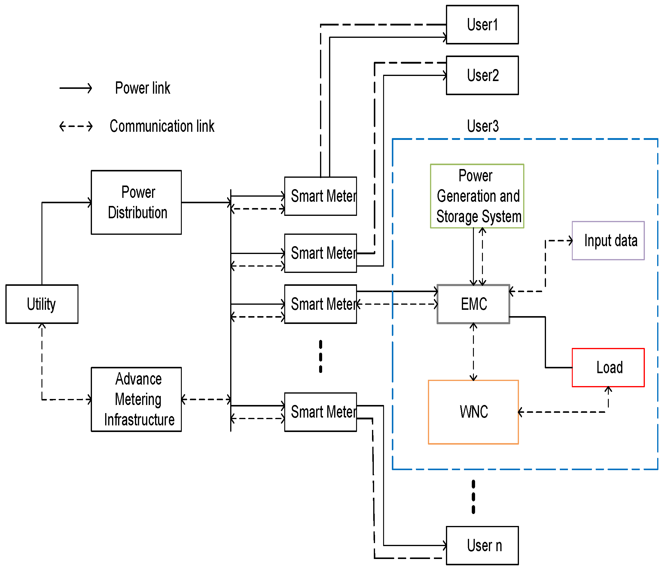
The review of relevant literature shows that homes equipped with Home energy management (HEM) architectures significantly reduce the electricity cost. HEMs equipped with renewable energy generation and storage architecture are given importance but the load matching with the renewable energy generation is ignored. Several HEM architectures efficiently shift the load from grid to an on-site energy generation and storage system, but the design of PV-based energy generation and storage setup has not yet been reported. An efficient and autonomous HEM architecture is required with twofold objectives, i.e., benefices the end user and utility. With the end user perspective, HEM needs to incorporate the on-site PV generation and storage system that optimally uses the grid and stored energy to maximize the comfort level. With the utility perspective, HEM should limit the energy consumption to a certain threshold level to avoid the load shedding, blackouts and use of peak power plants. Thus, our objectives are to design a demand side energy management (DSEM) model that (i) Categorizes, monitors and controls the household different loads according to end user preference and priority, (ii) Maximizes the end user comfort level by scheduling the load with minimum delay, (iii) Anticipates the optimum number of PV modules for an on-site load, i.e., smart home in our case, (iv) Efficiently integrates the PV generation and storage system with energy management controller (EMC), (v) Optimally manages the grid energy and on-site stored energy, (vi) Minimizes the end user electricity cost, (vii) Minimizes the PAR to increase the grid lifetime, avoid the blackout, load shedding and use of Peak Power Plants (PPPs), and (viii) Efficiently formulates and solves the optimization problem considering the constraints.

2. Literature Review

With rapid increase in energy demand and CO${}_2$ emissions due to massive use of fossil fuels, a significance attention needs to be given to consider renewable energy resources. Among all renewable energy resources, the most promising resources with nearly zero carbon emissions are the windmills and PV systems [39]. In comparison to both of the resources, energy obtained from PV system is highly attractive due to its abundant nature. Therefore, several incentive policies are designed especially for the end users to encourage them installing PV systems to alleviate uncertain energy demand during off peak hours. The integration of PV systems at end user side will reduce the energy cost, PAR, blackouts and carbon emissions, particularly. Consequently, PV systems tied with grid are expected to sustain popularity for the next generations [40]. One of the major challenges during the design of energy management systems (EMS) with the PV systems is its intermittent nature and thus leads to an increased design complexity. Other major challenges of PV system integration with existing electricity supply system are the variable PV generation and dynamic energy demand trends. The work reported in [41] used the on-site battery energy storage and PV system to solve the supply–demand mismatch problem. The work discussed in [42] focussed on efficient energy use for cost saving through an optimization algorithm with the integration of battery storage systems. The end user achieved the reduced energy cost by compromising on their comfort level. Thus, cost reduction and comfort maximization are contradictory objectives, hence difficult to achieve simultaneously.

Due to the battery-based ESS, autonomous control algorithms considering variable energy resources and dynamic energy demand are sought to optimally manage the available resources [43]. Therefore, combined dispatch and use of power resources considering a utility tariff scheme leads towards a complex optimization problem. Thus, finding the optimal charging and discharging patterns of battery storage system would ultimately minimize the end user electricity cost and maximize the power system stability. Numerous studies are available dealing with the complex nature of such types of problems and their possible solutions [44]. For nonlinear problems, it is less feasible to use mixed integer linear programming (MILP) and linear programming (LP) approaches without transforming the problem first [45]. The authors in [46] formulate the objective function using a binary and discrete decision variables with a low computing resources [47,48]. The authors in [49] used a hybrid computational intelligence approach for energy optimization using GA and Evolutionary algorithms. In this study, load is scheduled in such a way to minimize the electricity cost rebound peaks. Another study used ant colony optimization (ACO) algorithm to solve predefined load scheduling problem [50]. It is also concluded from the study that heuristic and metaheuristic algorithms such as; PSO, GA, ACO, are comparatively efficient in achieving the optimized solutions when uncertain decision variables are involved [51,52].

The extensive literature review regarding load scheduling has come up with individual technologies, policy recommendations, system analysis and control techniques, energy management, PV-based generation and storage integration issues [53]. Policy-based system analysis techniques sometimes tend to take statistical, qualitative and qualitative approaches while focusing on efficient resource management especially at residential premises [54]. Similarly, quantitative approaches have been case study driven and thus focusing on realistic solutions by taking into consideration utility and end user objectives. Some studies have a particular focus on devising customer centric solutions, while others tend to consider utilities concerns as well [55]. In the meantime, some researchers being able to devise autonomous energy management solutions considering utility and variable energy resources at the same time to facilitate both parties [56]. However, it is found that due to contradictory objectives, the solutions still have some gaps to be handled efficiently [57]. Another problem associated with some load management techniques is the single layer optimizations, such as; residential load scheduling [58], generation scheduling with distributed resources [59], optimal storage integrations [60], end user comfort management with particular focus on cost reduction [61]. Thus, due to lack of generic techniques considering respective objectives, most of these techniques neither feasible nor generally extensible to other case study geographies [62].

To complete the discussion, several researchers used different algorithms and energy management techniques to achieve energy saving and optimization objectives. Statistical results show that the building equipped with EMSs have energy saving factor from 11.39% to 16.22% each year. The EMS used for artificial lighting system reported the highest energy saving factor, of up to 39.5%. Similarly, the energy saving factor for HVAC and other equipments are reported as 14.07% and 16.66%, respectively. Furthermore, the published work also reported that EMS based on different optimization algorithms, such as the harmony search algorithm, enhanced differential evolution, and harmony search differential evolution, efficiently reduced the end user electricity cost by a factor of 17.84%, 11.12%, and 13.2%, respectively. Homes and buildings equipped with EMS architectures significantly reduce the electricity cost. However, EMS equipped with renewable energy generation and storage system and load matching with the PV generation system is not yet reported in the residential sector.

2.1. Contributions

The review of relevant literature shows that homes equipped with HEM architectures significantly reduce the electricity cost, although HEM equipped with renewable energy generation and storage units are given importance. However, the estimation of installed capacity of renewable and storage units as per load requirements is yet to be explored and significant work is required in this area. The literature reveals that HEM architectures efficiently manage the load considering grid and on-site energy generation and storage systems. However, the design of PV-based energy generation and storage systems need to be explored in order to get the full benefits of SG technology. Thus, an efficient and autonomous HEM architecture is required to provide benefits to both end user and utility. With the end user perspective, HEM needs to incorporate the on-site PV generation and storage system that optimally uses the grid and stored capacity to maximize the comfort level. With the utility perspective, HEM should be able to minimize the energy consumption to a certain level to avoid the load shedding, blackouts and use of expensive peak power plants. Thus, on the basis of aforementioned discussion, this work proposes a new home energy management (HEM) mechanism to address the limitations and drawbacks. The proposed work has the following capabilities; it facilitates the end users to decide whether they want to maximize comfort or cost (through a waiting time parameter), efficient load management with the integration of RES and user involvement significantly improved the power system stability through balanced supply–demand profile and it helps in reducing CO${}_2$ emissions as renewable energy and storage units act as “first choice” in the proposed work. The key contributions of this paper are discussed as follows:

• We first categorize the loads based on user preference requirement and priority of operation. Then based on this, mathematical models of each individualized load category are presented to help optimized working patterns.
• To facilitate end users in terms of less cost and high comfort, operational time of each load is modelled as a delay parameter, where high priority is given to critical load, while low priority loads are given flexibility in their operating horizon with the objective of minimized cost and delay.
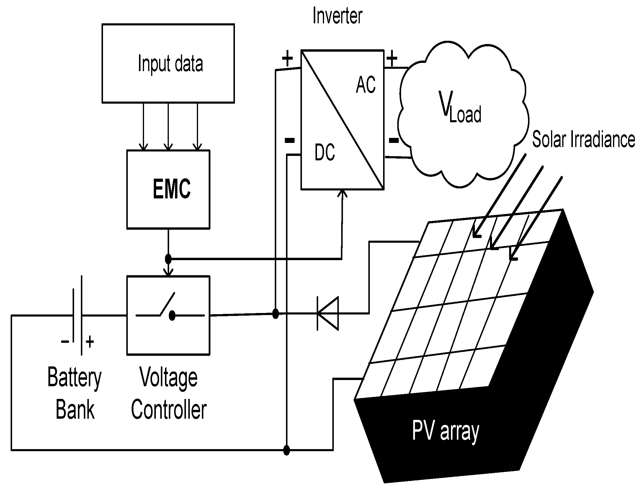
• To avoid users to buy costlier electricity tariff, on-site PV generation and back-up storage systems are integrated in our model. For this purpose, PV generation and storage systems are optimally designed in such a way to provide baseline load capacity to all respective loads without heavily relying on grid energy source. This helps in minimizing the cost and discomfort of end users along with reduced CO${}_2$ emissions.
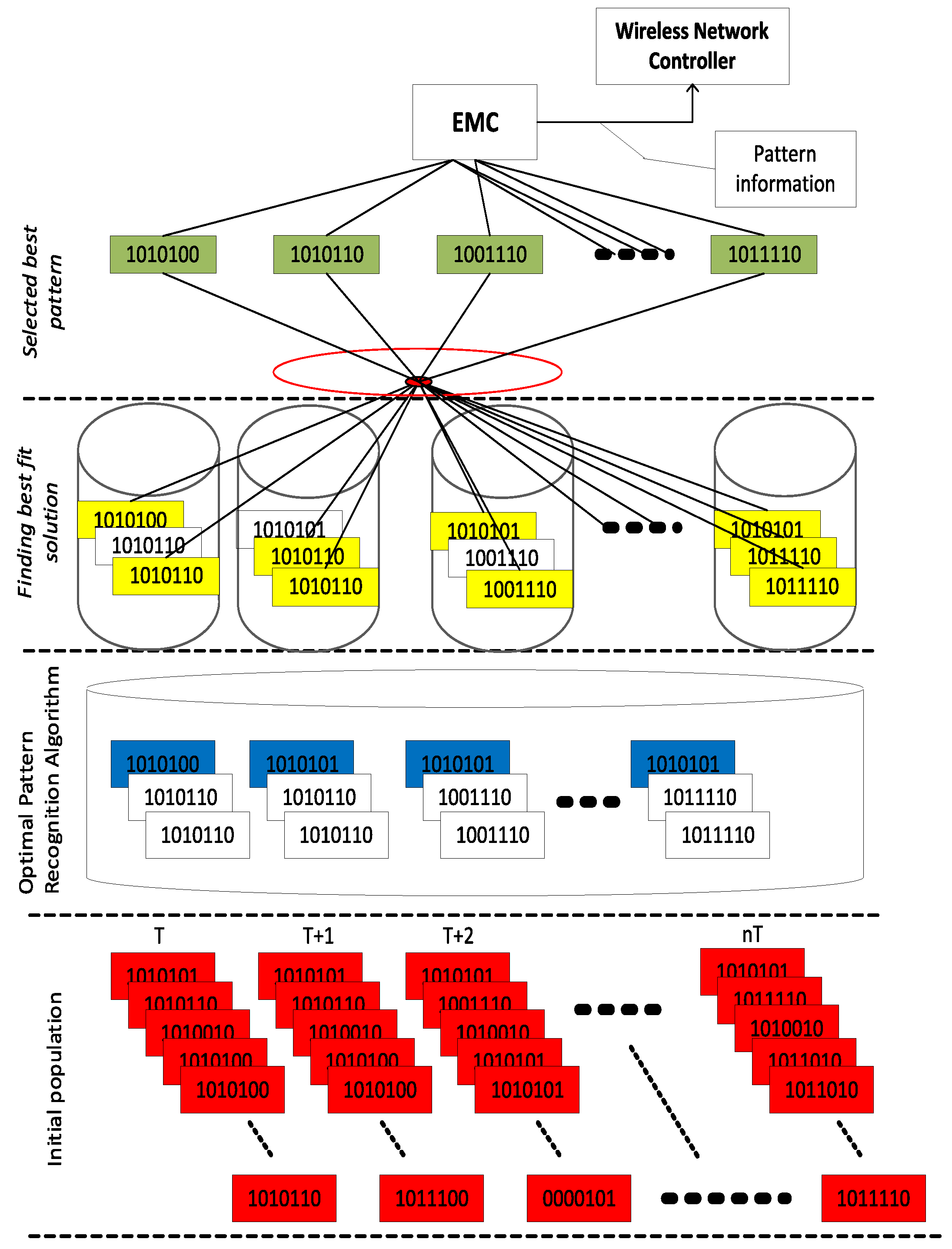
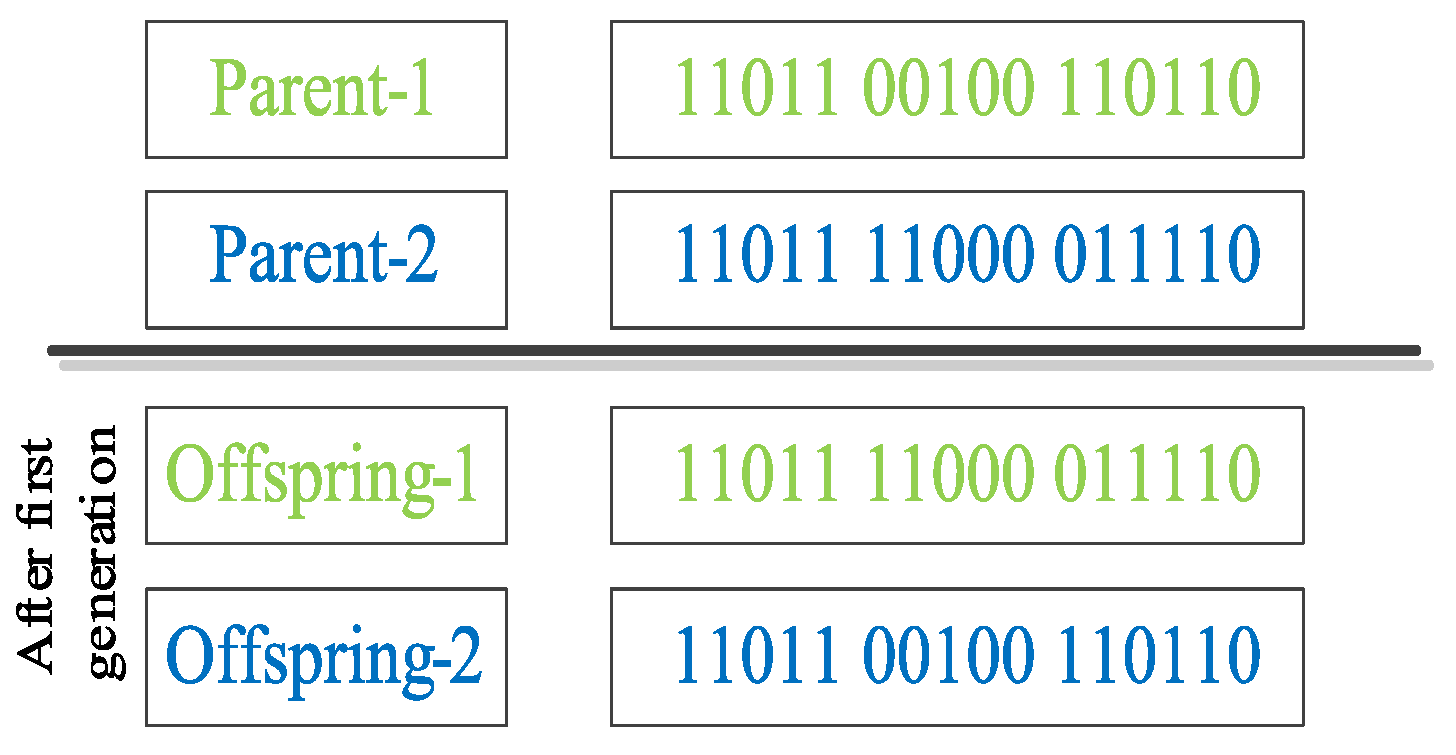
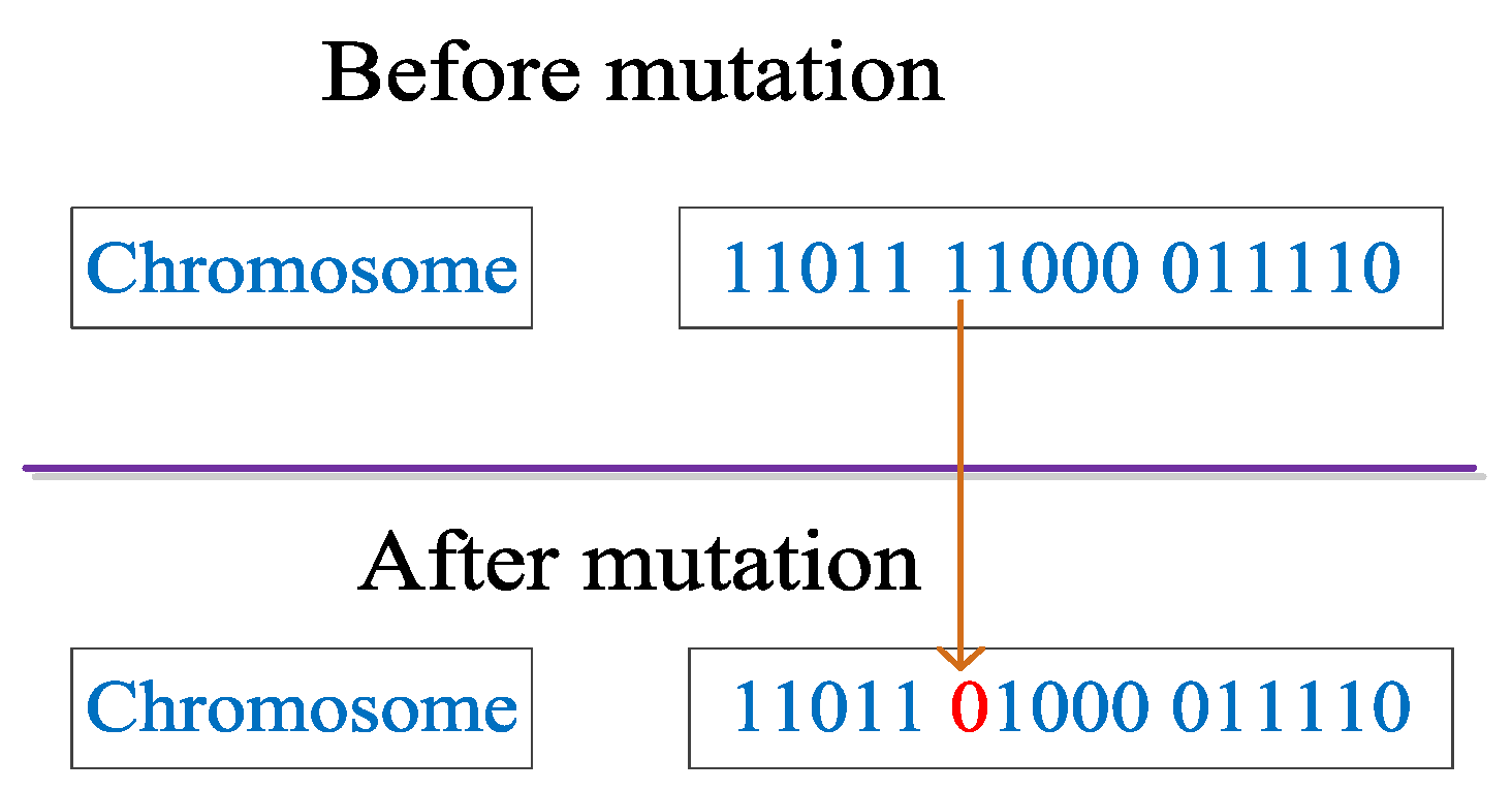
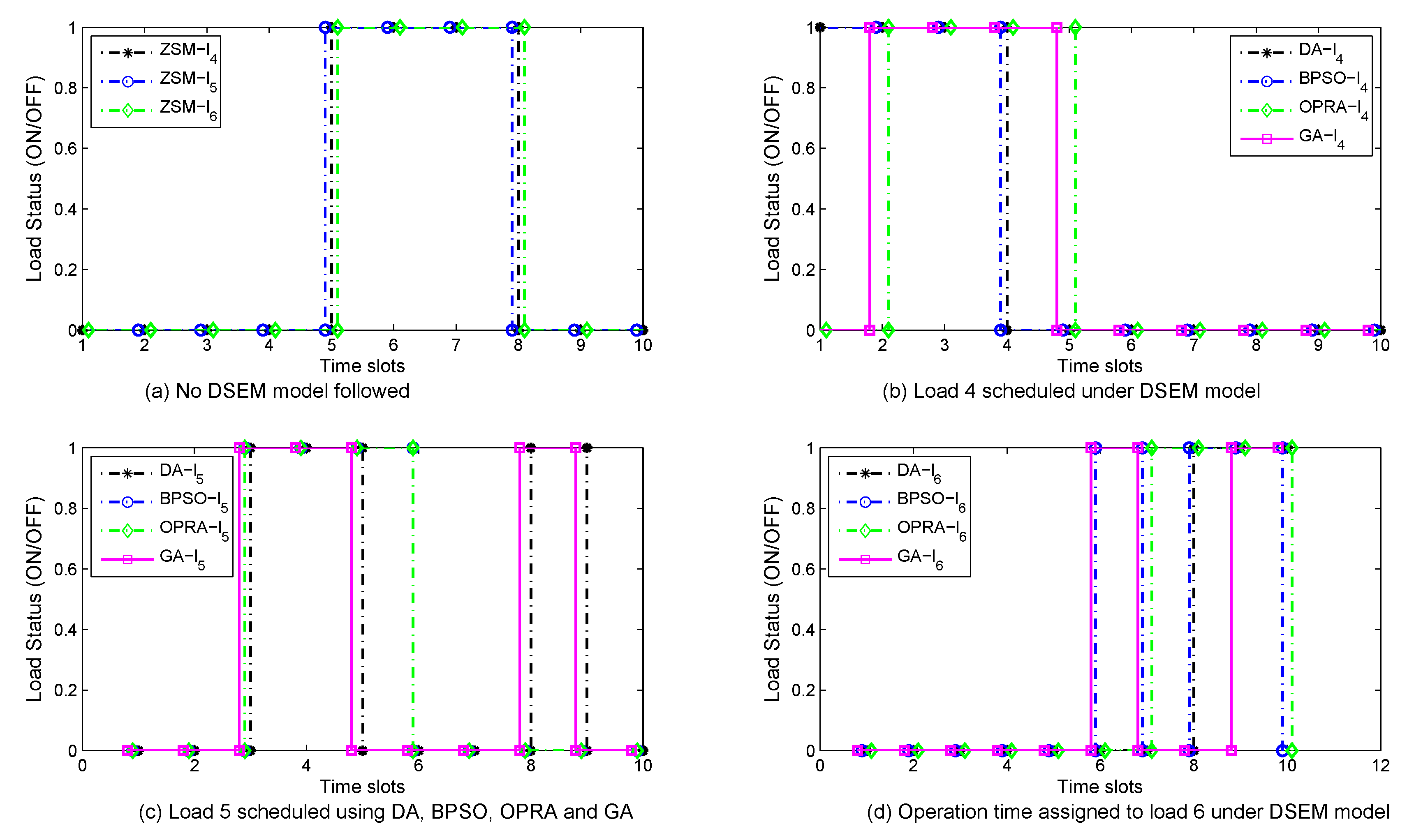
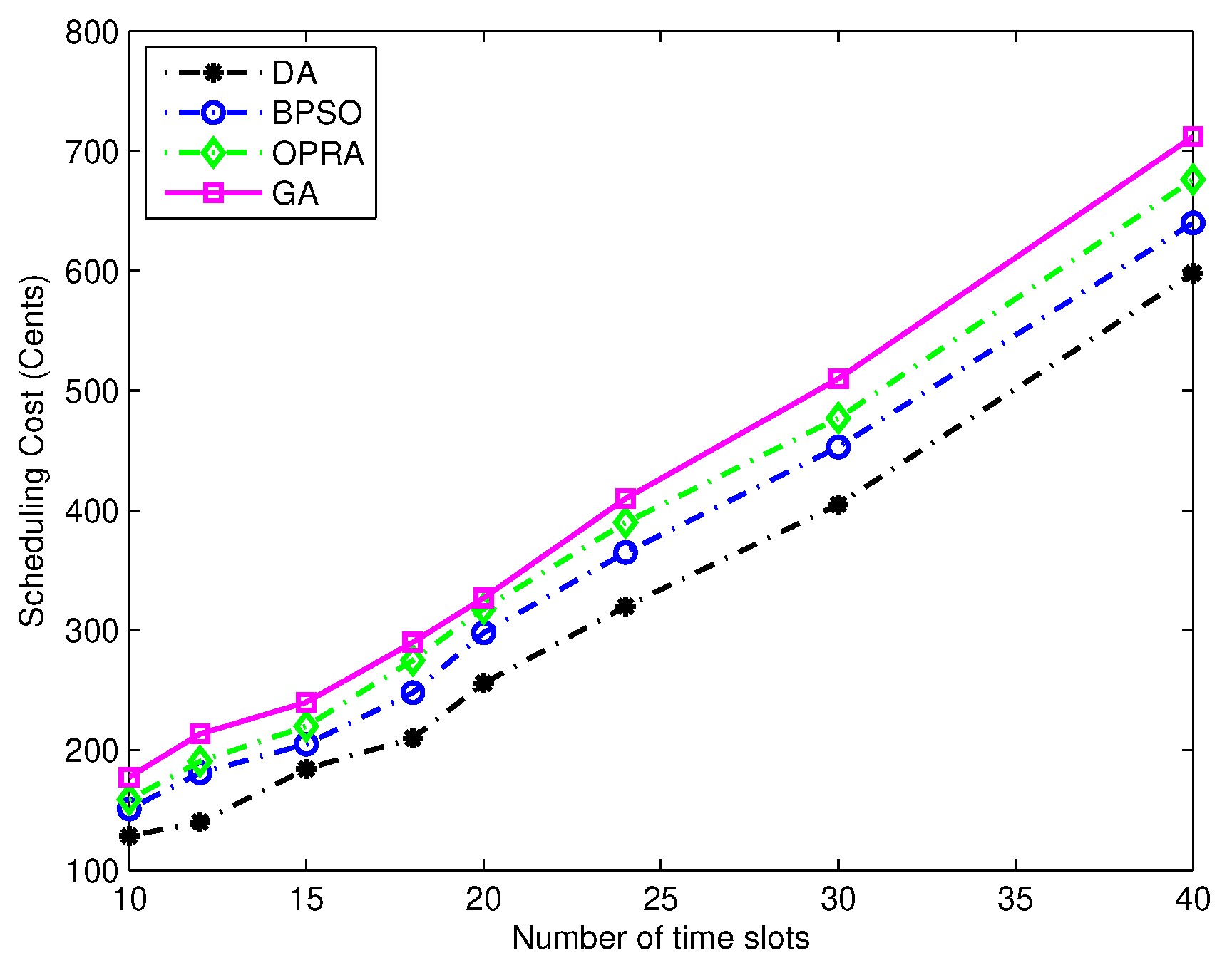
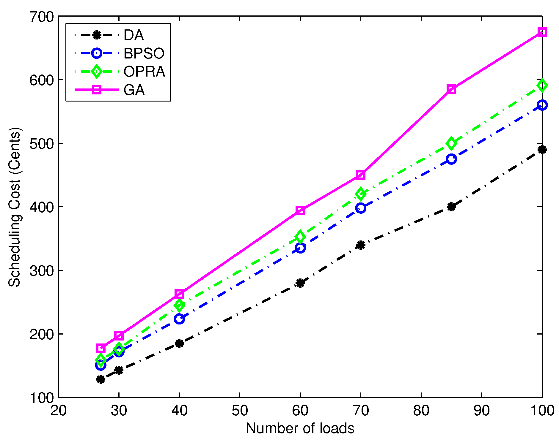
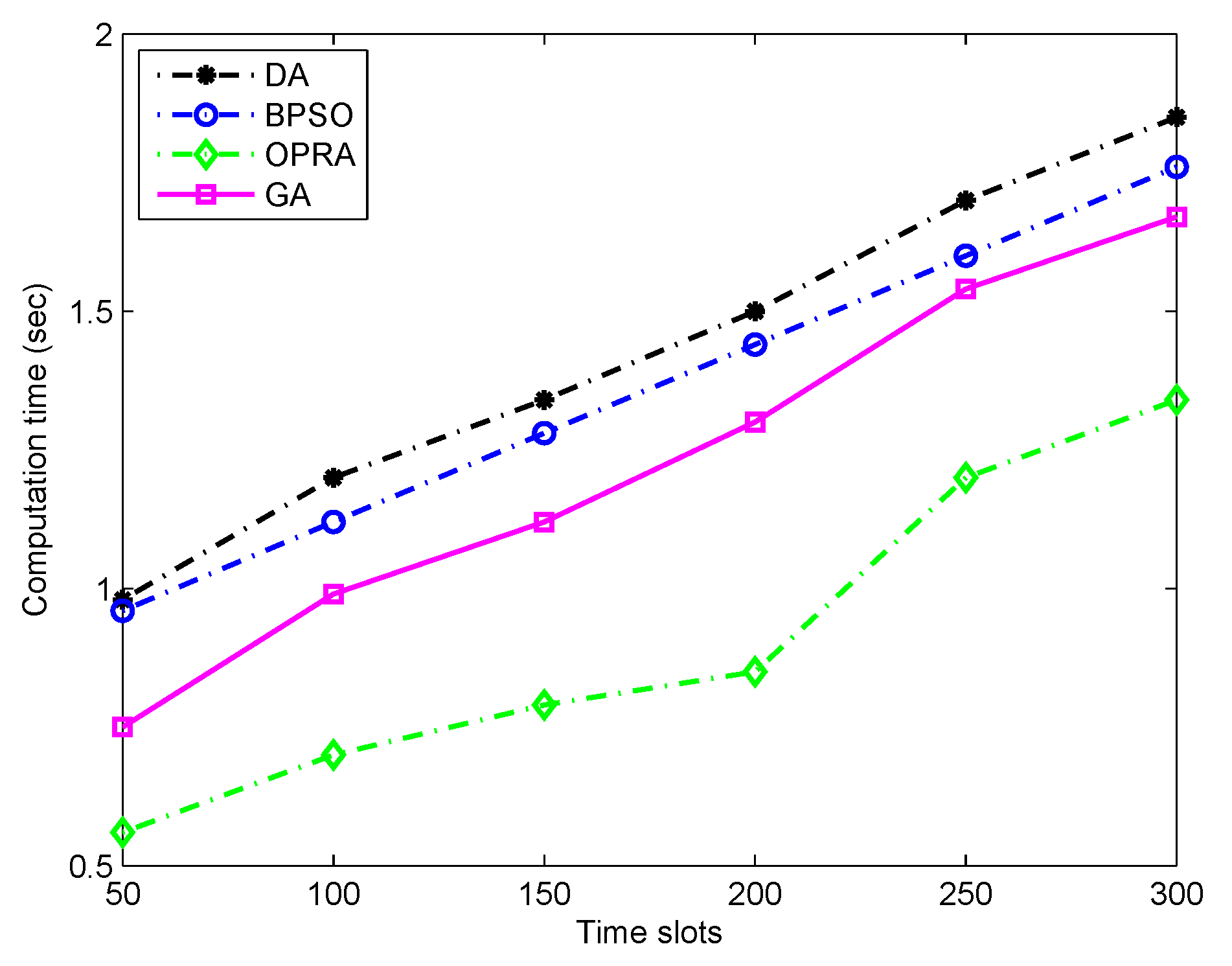
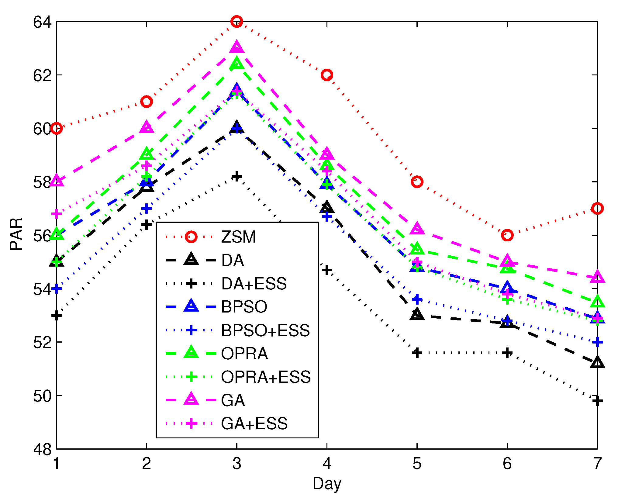
• Then based on mathematical models of load consumption, delay and ESS, the optimization problem is formulated as a multi-objective optimization problem which is solved by using DA. However, for optimality analysis, we compare the results of proposed DA with GA, BPSO and OPRA. Furthermore, the performance and complexity of the algorithms are also analysed in terms of large number of loads and time slot variations.
• The simulations are performed against different case studies and results are obtained for cost, PAR, CO${}_2$ and discomfort reduction.

2.2. Paper Outline

The rest of the paper is organized as: Section 3 discusses the DSEM model describing the mathematical description of different loads, on-site PV generation and storage systems, hybrid energy system and cost calculation mechanism. Section 4 presents the formulation of multi-objective optimization problem. Section 5 provides the description of different algorithms which are used to solve the proposed problem. Section 6 presents the results obtained from different algorithms focusing on load scheduling, cost and PAR reduction, optimal PV energy and storage integration and use. Finally, the paper is concluded in Section 7.

3. DSEM Model

The energy of a residential grid network is supplied by the utility and shared by several users through the power line. DSEM is equipped with EMC which is connected to household load on one side and smart meter on other side. The working of EMC is to: (i) collect the user preferences and demand information, (ii) send the control signal to each load via wireless network controller (WNC) for optimal consumption of energy, (iii) gather the energy generation and storage information from the on-site energy generation and ESS, (iv) optimally use the grid energy and ESS, and (v) receive the time variant electricity price signal from the utility. Based on the collected information, EMC sends an on-site energy demand to the smart meter. The smart meter bi-directionally communicates through communication line with the utility. The DSEM architecture is shown in Figure 1.

3.1. Modelling Consumption Behaviour

This section discusses the load consumption behaviour of the considered load. We also discuss the mathematical models of all load types and their respective constraints and limits. Let A denotes a set of automatic and manual operated residential loads such that:

$$\mathbf{A}=\mathbf{B}\cup \mathbf{C}\cup \mathbf{D}\cup \mathbf{E},$$

(1)

where, B, C, D and E represent sets of base, delay tolerant, semi delay tolerant and critical load, respectively. It is considered that B and E are zero-delay tolerant load, since the end user is not willing to give-up on the comfort level. The category C includes elastic loads in such that their operation time can be interrupted or shifted to any other time slot over the given time horizon $\mathcal{H}$. The category D comprises semi-delay tolerant loads that are assumed to be operated within a specific time window. The load in category E can be added any time as per user needs. The loads in B and E have the highest priority and zero tolerance towards delay. Moreover, the loads in D has the second highest priority and can bear some delay on the basis of predefined intervals $[{\alpha }_a,{\beta }_a]$. The category C is maximum delay tolerant and has the minimum priority. For each load a ∈ A, the power consumption vector over the given time horizon $t\in \mathcal{H}$ is written as;

$$P_{a,t}\triangleq [p_{a_1,t1},p_{a_2,t_2},\dots ,p_{a_n,\mathcal{H}}].$$

(2)

The loads in B, C, D and E consume certain amount of power during time t, can be written as:

$$\sum _{t=1}^{\mathcal{H}}\sum _{a\in \mathbf{A}}{P}_{a,t}\times {\sigma }_{a,t},$$

(3)

subject to:

$$\begin{array}{c}\underline{P_a}\le P_{a,t}\le \overline{P_a},\forall a\in \mathbf{A},\hfill \end{array}$$

(3a)

$$\begin{array}{c}{\sigma }_{a,t}=1,\forall t\in \{t_1,t_2,t_3\dots ,t_n\},\forall a\in \mathbf{B},\hfill \end{array}$$

(3b)

$$\begin{array}{c}{\sigma }_{a,t}=0,\forall t\in \mathcal{H}\setminus t,\forall a\in \mathbf{B},\hfill \end{array}$$

(3c)

$$\begin{array}{c}{\sigma }_{a,t}=1,\forall t\in {\mathcal{H}}^{{}^{\prime }},\forall a\in \mathbf{C},\hfill \end{array}$$

(3d)

$$\begin{array}{c}{\sigma }_{a,t}=0,\forall t\in \mathcal{H}\setminus {\mathcal{H}}^{{}^{\prime }},\forall a\in \mathbf{C},\hfill \end{array}$$

(3e)

$$\begin{array}{c}{\sigma }_{a,t}=1,\forall {\gamma }_a\le t\le {\delta }_a,\forall a\in \mathbf{E},\hfill \end{array}$$

(3f)

$$\begin{array}{c}{\sigma }_{a,t}=0,\forall t=\mathcal{H}-({\gamma }_a+l_a),\forall a\in \mathbf{E},\hfill \end{array}$$

(3g)

where, ${\sigma }_{a,t}$ is the status of load a during time slot t, $\underline{P_a}$ and $\overline{P_a}$ is the minimum and maximum power consumption, ${\gamma }_a$ is the operation start time, ${\delta }_a$ is the operation finish time, and $l_a$ is the length of operation time of load a. Equation (3a) gives upper and lower limits on power, while Equations  (3b)–(3f) denote power ON/OFF status of various loads according to the respective limits and conditions. The category E includes critical load, that can be plugged-in to the HEM architecture any time $\mathcal{H}$. The semi-delay tolerant load has a specific operation window e.g., for load $z_1$, the lower and upper bound are ${\underline{\mathrm{z}}}_1$ and ${\overline{\mathrm{z}}}_1$, respectively, in which load has to complete its task. The duration between ${\underline{\mathrm{z}}}_1$ and ${\overline{\mathrm{z}}}_1$ is divided as $[{\underline{\mathrm{z}}}_1,{\underline{\mathrm{z}}}_1+t]$, $[{\underline{\mathrm{z}}}_1+t,{\underline{\mathrm{z}}}_2]$, $[{\underline{\mathrm{z}}}_2,{\underline{\mathrm{z}}}_2+t]$, and $[{\underline{\mathrm{z}}}_2+t,{\overline{\mathrm{z}}}_1-t]$, and $[{\overline{\mathrm{z}}}_1-t,{\overline{\mathrm{z}}}_1]$. During the interval $[{\underline{\mathrm{z}}}_1,{\underline{\mathrm{z}}}_1+t]$,  $[{\underline{\mathrm{z}}}_1+t,{\underline{\mathrm{z}}}_2]$, $[{\underline{\mathrm{z}}}_2,{\underline{\mathrm{z}}}_2+t]$, and $[{\underline{\mathrm{z}}}_2+t,{\overline{\mathrm{z}}}_1-t]$, and $[{\overline{\mathrm{z}}}_1-t,{\overline{\mathrm{z}}}_1]$, the load may be either in ON or OFF state. After the time ${\overline{\mathrm{z}}}_1$, the load must be in OFF state. The power scheduling of load category D over the specified time range [${\alpha }_a$, ${\beta }_a$] is given as:

$$\begin{array}{c}{\alpha }_a\le t\le {\alpha }_a-{\beta }_a-{\rho }_a,\forall a\in \mathbf{D},t\in \mathcal{H}.\hfill \end{array}$$

(4)

where, ${\rho }_a$ gives the amount of time delay in regard when load is rescheduled to other feasible time slot during peak hours or overload conditions. The Equation (4) denotes that the load a∈D is restricted in between $\alpha$ and $\beta$ time intervals to complete its task. The allowed time horizon for any load a ∈ A should not be less than the length of its operation time and is expressed as:

$$l_a\le {\beta }_a-{\alpha }_a,\forall \mathcal{H}.$$

(5)

Then based on the aforementioned limits and constraints associated with respective load types, the information is transmitted to EMC via home area network as shown in Figure 2.

The operation start and finish time of load a ranges between $\gamma$ and $\delta$ and is calculated as:

$${\gamma }_a\le r_a\le {\delta }_a,\forall a\in \mathbf{A}$$

(6)

subject to:

$$\begin{array}{c}{\alpha }_a\le {\gamma }_a\le {\beta }_a-l_a,\hfill \end{array}$$

(6a)

$$\begin{array}{c}{\delta }_a\le {\beta }_a,\hfill \end{array}$$

(6b)

where, Equation (6a) gives the operation start time of ${\gamma }_a$ and Equation (6b) shows that each load must complete its task during allowed time horizon. Our objective is to optimize the power consumption vector of each load type over the given time interval. Therefore, in order to achieve this objective, the major emphasis is given to obtain optimized scheduling patterns of each load, especially elastic and semi elastic loads.

The category E has the highest priority and EMC needs to operate immediately whenever any service is required. EMC manages, monitors and controls the household loads and its working operation is shown in Figure 3.

Load Delay

It is usually expected that residential load can finish their working within the permissible time limits in order to avoid extra delay, which may disturb end user comfort level. Keeping this objective in mind, the maximum acceptable delay ($\overline{\rho }$) that any load can bear is calculated as:

$$\overline{{\rho }_{a,t}}=0,\forall a\in \{\mathbf{B},\mathbf{E}\},t\in \mathcal{H}$$

(7)

$$\overline{{\rho }_{a,t}}=\mathcal{H}-l_a,\forall a\in \mathbf{C},t\in \mathcal{H}$$

(8)

$$\overline{{\rho }_{a,t}}=({\beta }_a-{\alpha }_a)-l_a,\forall a\in \mathbf{D},t\in \mathcal{H}$$

(9)

whereas, the minimum delay ($\underline{\rho }$) for each load over the given time interval is:

$$\underline{{\rho }_{a,t}}=0,\forall a\in \mathbf{A},t\in \mathcal{H},$$

(10)

where, Equation (7) shows that load a belongs to the load category B and E and thus have zero tolerance towards delay, Equation (8) represents the load category C that has the minimum priority and can be scheduled anytime in the entire time horizon and Equation (9) shows that load a belongs to the semi-delay tolerant category and can only be scheduled in the pre-set allowed time slots. Where, ${\Gamma }_{req,a}$ denotes the required operation time of load a, and ${\Gamma }_{EM{C}_a}$ provides the scheduled time interval. Hence, Equation (10) elucidates that scheduled time interval is equal to the required amount of time needed to perform a specific task.

$${\Gamma }_{req,a}={\Gamma }_{EM{C}_a}$$

(11)

Therefore, in order to achieve this objective, EMC seeks to minimize the mismatch between required and optimized time intervals in association with limits and constraints.

3.2. On-Site Energy Generation and Storage System

In communication and networks, the coexistence of both discrete and continuous valued agents is interpreted as hybrid system [9]. Whereas in SG, a hybrid energy system is defined as the existence of more than one energy system to accommodate the end users energy demand. As was discussed, total load demand is fulfilled by the grid, renewable energy and storage systems and this complete architecture is considered to be a hybrid energy system, wherein renewable energy and battery storage systems act as “primary choice”, while the grid source acts as secondary choice in fulfilling the energy demand. In doing so, the end user can enjoy the reduced electricity cost, while utility gains the benefits in terms of power system stability as high peaks are eliminated during demanding hours. This proposed system architecture is shown in Figure 4.

3.2.1. PV Generation

The average power obtained from installed PV modules is calculated as:

$${\kappa }_{avg}=P_i\times {\varsigma }_i,$$

(12)

where, $P_i$ denotes the power produced by PV cell at irradiance level i and ${\varsigma }_i$ gives the probability of irradiance. The Equation (12) for irradiance spectrum can be written as [46]:

$${\kappa }_{avg,t}=\int P_{i,t}\times {\varsigma }_{i,t}dt,\forall t\in \mathcal{H},$$

(13)

The Equation (13) denotes the average power output of a PV module for all the possible irradiance spectrums in the integral form. Where, $P_{i,t}$ can be written in terms of voltage V and current I as under:

$$P_{i,t}=V_{i,t}\times I_{i,t},\forall t\in \mathcal{H}.$$

(14)

The Equation (14) gives average power obtained form PV array against specific temperature and irradiance over the given time t. Thus, the total obtained power as per dynamic temperature and irradiance can be calculated using [63,64,65]. Whereas, the rate of change in temperature with respect to the reference temperature is calculated as:

$$\delta T=T-T_r$$

(15)

Equation (16) gives the rate of change in current due to variation in PV module tilt and temperature:

$$\delta I=a\times \left(\frac{S}{S_r}\right)\times \delta T+\left(\frac{S-S_r}{S_r}\right)\times I_{sc}$$

(16)

Equation (17) is the change in voltage due to change in current during different time horizon:

$$\delta V=-b\times \delta T-R_s\times \delta I$$

(17)

This rate of change results in changing the value of V and I, which are given as:

$$V_{new}=V_r+\delta V$$

(18)

$$I_{new}=I_r+\delta I$$

(19)

The insolation and cell temperature level relation is defined as the sum of ambient temperature and two percent of the irradiance level and is given as under:

$$T=\frac{s}{50}+T_A$$

(20)

The optimum number of PV modules required for the household maximum load shifted from grid to ESS at any time slot t is anticipated as: if n${\kappa }_t<P_{D,t}$, increase the value of n. The quality of load matching depends on PV arrays, load characteristics, and isolation profile. Based on PV supply/demand match evaluation criteria, an optimum PV-site matching technique is used to select the module type with the highest average capacity and lowest cost. The current I of the PV module as a function of V can be expressed as [66]:

$$I=I_{sc}\left\{1-g_1\left[e^{\left(g_2{V}^n\right)}-1\right]\right\}$$

(21)

The values of constants, $g_1$, $g_3$ and n are obtained from [63]. Finally, the total renewable energy ${\kappa }_{tot,t}$ obtained from PV system is used in two ways; some amount ${\kappa }_{a,t}$ is directly provided to fulfil the residential load demand, while, the remaining energy $({\kappa }_{{st}_{s,t}}={\kappa }_{tot,t}-{\kappa }_{a,t})$ is stored in backup storage system. The relationship between these two amounts is given as:

$$\sum _{t=1}^{\mathcal{H}}\left(\sum _{a\in \mathbf{A}}{\kappa }_{a,t}+\sum _{s=1}^N{\kappa }_{{st}_{s,t}}\right)\le {\kappa }_{tot,t}$$

(22)

In contrast to renewable energy, the net amount of energy obtained from grid at any time slot $t\in \mathcal{H}$ cannot exceed a certain level $P_{max}^{grid}$, which is given as:

$$\left(\sum _{t=1}^{\mathcal{H}}\sum _{a\in \mathbf{A}}{P}_{a,t}+P_{c_{s,t}}\right)-{\kappa }_{s{t}_{s,t}}\le P_{max}^{grid},\forall {\sigma }_{a,t}=1$$

(23)

where, $P_{c_s,t}$ denotes the electrical charge in the battery power. Furthermore, the ESS must satisfy Equation (24) constraint for any type of load that is to be shifted from the grid to ESS:

$${\kappa }_{s{t}_{s,t}}-(P_{a,t}\times {\sigma }_{a,t})\ge 0,\forall a\in \mathbf{A},\forall 1\le t\le \mathcal{H}.$$

(24)

where, the remaining power obtained from PV generation must not exceed the ESS capacity:

$$P_{c_{s,t}}-{\kappa }_{{st}_{s,t}}\ge 0,\forall s,t\in \mathcal{H}.$$

(25)

3.2.2. ESS

As it is understood, ESS has the upper and lower levels to store the surplus energy, which is expressed as:

$$\underline{\kappa L_{s,t}}\le \kappa L_{s,t}\le \overline{\kappa L_{s,t}}\forall 1\le t\le \mathcal{H}.$$

(26)

The total amount of surplus energy which can be stored in ESS at time t, which is greater than $\kappa L_{s,I}$ is given as:

$$\left(\kappa L_{s,t}=\kappa L_{s,t-1}+(P_{c_{s,t}}\times {\eta }_s)-\frac{P_{d_{s,t}}}{{\eta }_s}\right)\ge \kappa L_{s,I}\forall t\in \mathcal{H}.$$

(27)

where, ${\eta }_s$, $P_{d_{s,t}}$ and I denote efficiency of battery s, discharge in power of the battery and pre-defined storage quantity, respectively. To prolong the battery life time, it is recommended to avoid deep discharge of a battery. Therefore, we defined upper and lower limits on battery charge and discharge rate, which are given as:

$$\underline{P_{c_{s,t}}}\le P_{c_{s,t}}\le \overline{P_{c_{s,t}}},\forall t\in \mathcal{H}.$$

(28)

$$\underline{P_{d_{s,t}}}\le P_{d_{s,t}}\le \overline{P_{d_{s,t}}},\forall t\in \mathcal{H}.$$

(29)

During the time when load demand exceeds a certain level and electricity tariff is also high, then ESS acts as “first choice” to fulfil the load demand. Therefore, ESS starts providing the energy as per schedules given by EMC and is given as:

$${\kappa }_{s{t}_{s,t+1}}={\kappa }_{s{t}_{s,t}}-P_{d_{s,t}},\forall t\in \mathcal{H}$$

(30)

whereas,

$$P_{d_{s,t}}=\sum _{a\in \mathbf{A}}(P_{a,t}\times {\sigma }_{a,t}),\forall t\in \mathcal{H}$$

(31)

The Equation (30) denotes the remaining stored energy in the ESS system. Whereas, the Equation (31) represents the amount of energy dissipated during time slot t for the load a ∈$\mathbf{A}$ shifted from grid to ESS system.

3.2.3. Evaluation of Hybrid Energy System

The daily load demand of the end user as a function of t and user preferences are shown in Table 2.  End users are hoping to fulfil their demand using PV system, ESS and grid resources. Whereas, the choices to use these resources are mentioned above. Therefore, in order to manage these energy resources efficiently, with the objective of overall cost reduction and power system stability, autonomous energy management algorithm is needed. In this regards, this work considers all the objectives and limitations and designs an autonomous load scheduling algorithm(s). As the primary source of energy is PV and ESS system, therefore, the total PV modules required to fulfil the load demand and the energy obtained from the grid are calculated as:

$$j_{pv}\times P_{o,t}\times {\varphi }_{pv}=P_{D,t}$$

(32)

$$P_{g,t}\times {\varphi }_g=P_{D,t}$$

(33)

where, $j_{pv}$ denotes the total number of PV modules required for the energy demand D, ${\varphi }_{pv}$ and ${\varphi }_g$ define efficiency of PV modules and grid system, and $P_{o,t}$ and $P_{g,t}$ are power imported from single PV module and grid at time slot t, respectively. The equation formulated for a hybrid energy system is given as:

$$z\times P_{o,t}\times {\varphi }_{pv}+(1-z)P_{g,t}\times {\varphi }_g=P_{D,t},$$

(34)

where, z denotes the ratio which is used to define the amount of PV and grid energy. The best fit ratio z is anticipated by using LSM and is given as [64]:

$$\begin{array}{c}\hfill z_{bf}={\left[{({\varphi }_{pv}\times P_{o,t}-{\varphi }_g\times P_{g,t})}^t({\varphi }_{pv}\times P_{o,t}-{\varphi }_g{P}_{g,t})\right]}^{-1}\times {({\varphi }_{pv}\times P_{o,t}-{\varphi }_g{P}_{g,t})}^t(P_{D,t}-({\varphi }_g\times P_{g,t}))\end{array}$$

(35)

It reduces the sum of squares of deviations of generated power and household load, which is expressed as [64,65,66]:

$$({\varphi }_{pv}\times P_{o,t}-{\varphi }_g\times P_{g,t})\times z=P_{D,t}-({\varphi }_g\times P_{g,t})$$

(36)

Based on Equations (35) and (36), EMC takes decision about when to use ESS along with grid energy. For example, if $0<z<1$, then it would be beneficial to usde ESS along with grid energy.

3.3. Energy Consumption and PAR Model

For each load a ∈ A, the energy consumed by load is given as:

$$E_{a,t}=\sum _{t={\gamma }_a}^{{\delta }_a-\rho }\sum _{a\in \mathbf{A}}{P}_{a,t}\times {\sigma }_{a,t}\times l_a,\forall {\sigma }_{a,t}=1.$$

(37)

Let the house have N number of loads, then the total daily energy demand $E_{tot,t}$ of a single household is written as:

$$E_{tot,t}=\sum _{t=1}^{\mathcal{H}}\sum _{a\in \mathbf{A}}{E}_{a,t}\times {\vartheta }_{a,t}.$$

(38)

where, ${\vartheta }_{a,t}$ is the operation time of load a during time slot t. Generally, if we consider only the users’ benefits, then the load scheduling has to be performed in a way that most of the load during high peak hours will be shifted to off-peak hours leading towards reduced billing cost. However, it may create rebound peaks which ultimately disturb power system stability regarding high PAR. In contrast, the effective load management mechanism has to reschedule the load to avoid the rebound peaks. Otherwise, the energy retailers and service providers keep backup generation capacity to protect electrical network. Eventually, this may lead costlier generation and hence increase the tariff price which would ultimately disturb end user benefits. Mathematically, the PAR is calculated as follows:

$$PAR=\frac{\overline{P}}{P_{avg}}$$

(39)

where,

$$\overline{P}=ma{x}_{t\in \mathcal{H}}\left(\sum _{t=1}^{\mathcal{H}}\sum _{a\in \mathbf{A}}{P}_{a,t}\right)$$

(40)

and

$$P_{avg}=\frac{{\sum }_{t=1}^{\mathcal{H}}{\sum }_{a\in \mathbf{A}}{P}_{a,t}}{\mathcal{H}}.$$

(41)

Equation (39) shows the ratio between the maximum power and average power consumed by household load a at a given time horizon $\mathcal{H}$. An efficient energy consumption leads to a minimized PAR and thus our third objective is to minimize the maximum PAR over the given time slot.

3.4. Cost Model

The daily energy consumption cost of N household loads during time slot $t\in \mathcal{H}$ is calculated by EMC as:

$$C_{1,t}\triangleq \sum _{t=1}^{\mathcal{H}}\sum _{a\in \mathbf{A}}([P_{a,t}\times l_{a,t}]\times {\sigma }_{a,t})\times {\psi }_t,\forall {\sigma }_{a,t}=1.$$

(42)

where, ${\psi }_t$ is the electricity cost charged by the utility for the amount of energy consumed at time slot t. It is, therefore, reasonable to assume that the total cost anticipated by utility for load a∈$\mathbf{A}$ would become:

$$C_{2,t}=\sum _{t=1}^{\mathcal{H}}\sum _{a\in \mathbf{A}}{E}_{tot,t}\times {\psi }_t.$$

(43)

Now, the fair billing $\mathcal{B}$ is defined as:

$$\mathcal{B}\triangleq \frac{{\sum }_{t=1}^{\mathcal{H}}{C}_{2,t}}{{\sum }_{t=1}^{\mathcal{H}}{C}_{1,t}}\ge 1.$$

(44)

The fair billing is validated by the end user if $\mathcal{B}=1$, and if $\mathcal{B}>1$, then user’s bill includes the cost ${\mathcal{E}}_{cost}$ due the losses that occurred in between power distribution and smart meter at any time t and is calculated by:

$${\mathcal{E}}_{cost,t}=C_{2,t}-C_{1,t},\forall t\in \mathcal{H}$$

(45)

4. Formulation of Multi-Objective Optimization Problem

The objective of proposed model is to optimally schedule the household load over the given time period by taking into consideration respective constraints and limits. In this regard, the proposed algorithm is designed to optimally integrate PV system, ESS, and grid energy resources with the objective of cost and PAR reduction with increased comfort level. Hence, the primary objective is to fulfil the load demand through PV and ESS system without heavily relying on grid energy source.

$$\mathit{P}\mathit{1}=minimize\left\{\sum _{t=1}^{\mathcal{H}}\sum _{a\in \mathbf{A}}\left([P_{a,t}\times {\vartheta }_{a,t}]-{\kappa }_{tot,t}\right)\right\}.$$

(46)

subject to:

$$0\le \overline{{\rho }_a}\le {\delta }_a-{\gamma }_a-l_a,\forall a\in \mathbf{A}$$

(47)

$${\alpha }_a\le {\vartheta }_a\le {\beta }_a,\forall a\in \mathbf{A}$$

(48)

$$\begin{array}{c}\hfill E_{a,t}=\left\{\begin{array}{c}{P}_{a,t},t_a\in {\delta }_a-{\gamma }_a-{\rho }_a,\forall a\in \mathbf{A},t\in \mathcal{H},\hfill \\ 0,\mathcal{H}\setminus t_a\hfill \end{array}\right.\end{array}$$

(49)

$${\sigma }_{t,a}\in \{0,1\}$$

(50)

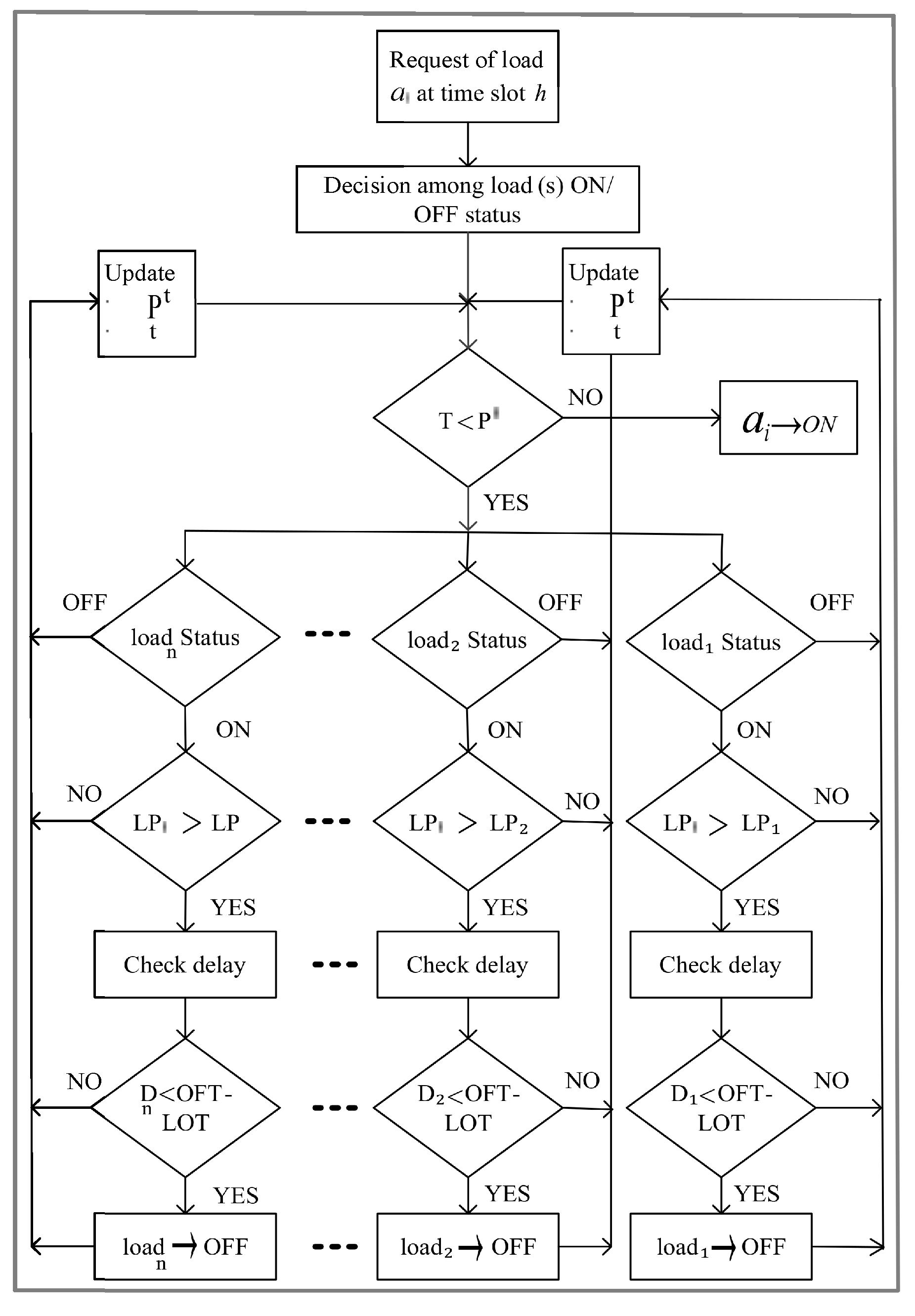
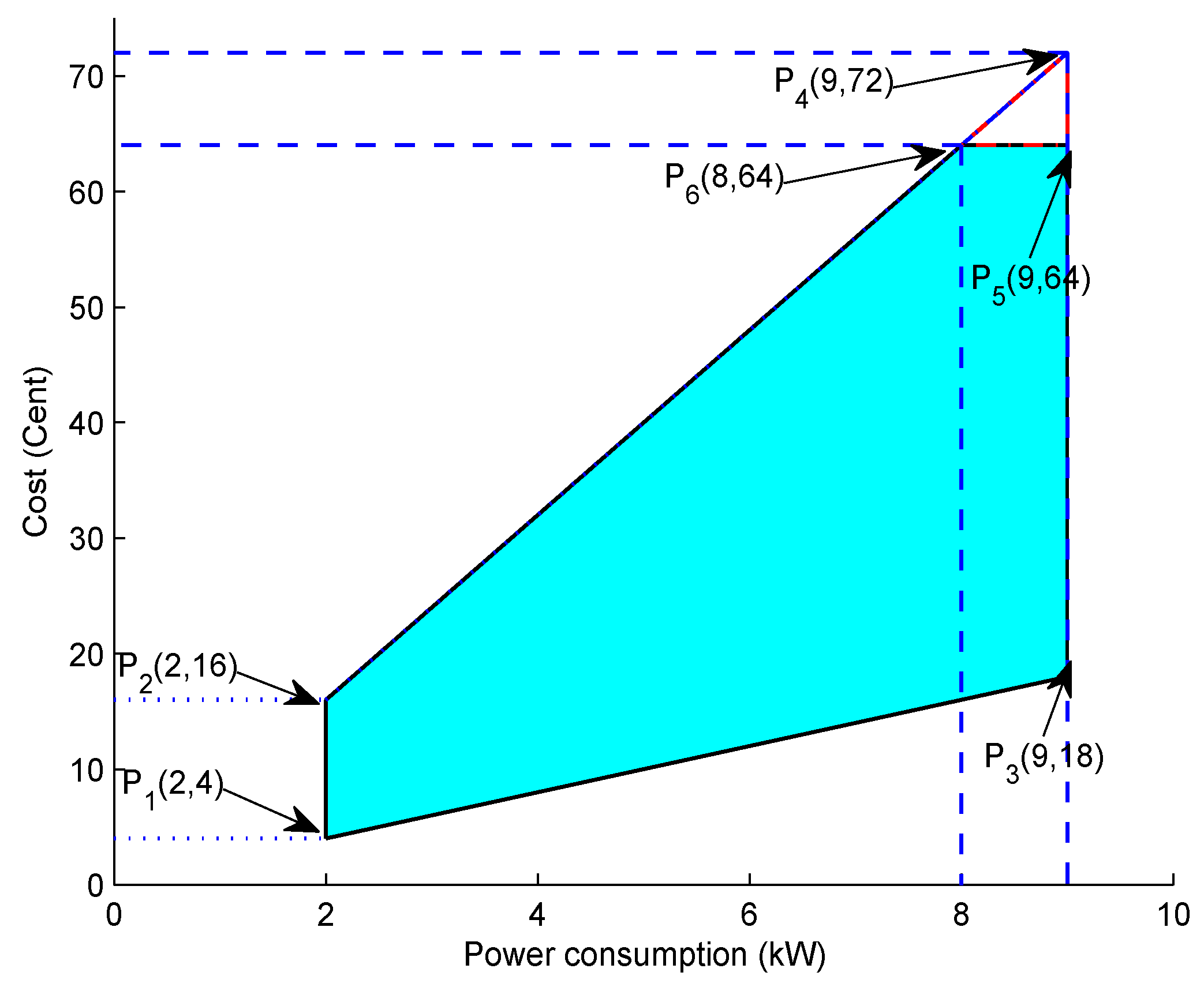
The constraints shown in Equations (47)–(50) define: (i) maximum load delay between starting and finish time while completing its task, (ii) load a must complete its assigned task within the allowed time ($\alpha$ and $\beta$), (iii) load a consumes certain amount of power during its operation time, and (iv) status of the load a (0 for idle mode, 1 for operation mode).

Therefore, the optimal management and use of the energy resources lead to effective cost minimization, because the electricity prices are dynamic in nature and usually known in advance to customers in a day-ahead market. However, prices are unknown to users in a real time pricing (RTP) environment, where it is more difficult to optimally manage the loads in conjunction with the integration of distributed energy resources (PV and ESS). Therefore, our next objective is to reduce the electricity cost through scheduling the load in optimal time slots without curtailing the load demand and is given as:

$$\mathit{P}\mathit{2}=minimize\{\sum _{t=1}^{\mathcal{H}}\sum _{a\in \mathbf{A}}\left([P_{a,t}\times {\vartheta }_{a,t}]-{\kappa }_{tot,t}\right)\times {\psi }_t\}.$$

(51)

where, Equation (51) denotes the electricity cost charged by the utility against the amount of energy consumed by load a during time slot t. However, it is worth mentioning here that in order to avoid the situations when high peak can be generated due to turning-on high load during low pricing hours, a threshold is imposed to limit the maximum upper limit of energy consumption. Thus, an efficient energy consumption leads to a minimized PAR and thus our next objective is to minimize the maximum PAR over the given time slot t and is formulated as:

$$\mathit{P}\mathit{3}=minimize\left(PAR\right)$$

(52)

subject to:

$$\sum _{t=1}^{\mathcal{H}}\sum _{a\in \mathbf{A}}{P}_{a,t}\le {\tau }_{max}.$$

(53)

where, ${\tau }_{max}$ is the threshold value used to avoid different risks, such as blackout, use of expensive backup generation plants, and load shedding. Generally, each user has a desire to complete the tasks of each load with minimum delay subject to minimized electricity bill. Thus, our next objective is to minimize the load operation delay in order to achieve maximum end user comfort and is described as:

$$\mathit{P}\mathit{4}=minimize\left\{\sum _{t=1}^{\mathcal{H}}\sum _{a\in \mathbf{A}}{\rho }_{a,t}\right\}.$$

(54)

subject to:

$${\rho }_{a,t}=\mathcal{H}-l_a,\forall a\in \mathbf{C},t\in \mathcal{H}$$

(55)

$${\rho }_{a,t}=({\beta }_a-{\alpha }_a)-l_a,\forall a\in \mathbf{D},t\in \mathcal{H}$$

(56)

$${\rho }_{a,t}=0,\forall a\in \left\{\mathbf{B},\mathbf{E}\right\},t\in \mathcal{H}$$

(57)

The constraints in Equations (55)–(57) define the allowed scheduling horizon for each load a ∈$\mathbf{A}$.

Mathematically, the cost minimization objective function in conjunction with PV and ESS integration is written as:

$$\begin{array}{c}\hfill \mathit{P}\mathit{5}=minimize\left(P1+P2+P3+P4\right).\\ \hfill subjectto:Equations\left(7\right)–\left(11\right),\left(28\right),\left(29\right),\left(47\right)–\left(50\right)\end{array}$$

(58)

5. Proposed Solutions

In the following sections, we describe the working and coping of the algorithms used to solve the multi-objective optimization problem. For detailed analysis, we used heuristic and robust optimization algorithms and provided the merits and demerits on the basis of input and outputs.

5.1. Optimal Load Scheduling Using DA

DA is a greedy graph search algorithm that is used to find the shortest path for load scheduling problems in micro grid [56,67,68]. It calculates the shortest path (with lowest cost in our case) for a start point (source node; operation start time of load) to the end point (destination node; finish time of load) in the graph. The DA anticipates the shortest path, i.e., minimum cost from any specific source node $s_1$ to any node in a parent weighted graph such as; $G_w=(\mathbf{F},\mathbf{e})$, where F and e are the sets of vertices and edges, respectively. Initially, the algorithm calculates weights as it traverses from the source node to all the connected nodes and saves the best values. Then it moves through all other connected nodes to find the next best value. Meanwhile, it also avoids saving all the previously saved best value and calculates the cost by comparing with previously saved values. The weighting factor x is the sum of edges weights from the node $s_1$ to d and is given as:

$$\begin{array}{c}\hfill if(u,f)\subset \mathbf{e}\to x(u,f)>0\forall f,u\in \mathbf{F}\\ \hfill x(f_1,f_2,\dots ,f_n)=\sum _{i=0}^{i=1}x(f_i,f_{i+1})\end{array}$$

(59)

where, $x(f_i,f_{i+1})$ is the weight (cost) between $f_i$ and $f_{i+1}$. The shortest path from u to f, $d(u,f)$, in G has the minimum weight among all nodes. If there is no path between u and f, then $d(u,f)=\infty$.

$$\begin{array}{c}\hfill \mathbf{S}=\left\{u\right|u\in \mathbf{F}\}\\ \hfill f\in \mathbf{F}\to f(u,f)isdefined,\forall u\in \mathbf{S}\end{array}$$

(60)

where, S is a subset of F, made-up gradually in an iterative process as follows: (a) start node y is selected from set F and inserted in S, (b) the shortest path from y to all available nodes in set $\mathbf{F}-\mathbf{S}$ are determined as:

$$\begin{array}{c}\hfill d(y,f)=d(y,u)+min\left[x\right(u,f\left)\right],\forall f\in \mathbf{F}\setminus \mathbf{S}\end{array}$$

(61)

where, u is the node between f and y. In the next step, the marked best fit solution u and the related edges to this node are added to set S and e, respectively. The algorithm continues until it updates all the nodes in set S, which means the final result is achieved. The time complexity of DA is $\left(O\right(N+N(N-1)+N(N-1)(N-2)+\dots +N(N-1)(N-2)\dots (N-N-1)\left)\right)$. The pseudo-code of DA is shown in Algorithm 1.

Algorithm 1 DSEM model based on DA.

Require:$a,b,s,d,g$ 1: $d_a=0,g\ge 0,P_a=\infty ,\forall a\in \{1,2,3,\dots ,N\}$ 2: $T_c=mini(g,1),\%T_c\to currentTier$ 3: $T_c++$ 4: $T_n=mini(g,T_c)$, $T{N}_c=d_1,d_2,d_3,\dots ,d_N$; %  $T{N}_c\to$  current TierNode 5: $T{N}_n=\infty$ 6: Find $e=argmin{i}_a\left(d_e^{d_a}\right)$ 7: Update P = P  $\cup d_e;\%P\to Path$ 8: $T{N}_n=T{N}_c-\left\{d_e\right\}$; 9: while$T{N}_c\ne \infty$do 10:   $T{N}_c=T{N}_n$; 11:   $s=d_e;\%d\to$  Destination 12:   $e=argmini\left(d_s^{d_a}\right);\forall d_a\in T{N}_n$ 13:    Update P = P $\cup d_e$; 14:   $T{N}_n=T{N}_c-\left\{d_e\right\}$ 15: end while 16: $P_r$ is obtained; %  $P_r\to$ resultant Path

5.2. Optimal Load Scheduling Using BPSO

BPSO is a population-based heuristic optimization technique used in micro grid for load scheduling [69,70,71] in which each possible solution in entire search space is represented by a particle. Initially, each particle is assigned a random position and velocity. Each particle represents the status of the electrical load. In this work, a pattern of n number of particles is selected that represents the n number of household electrical loads. For example, if the household has 10 electrical loads then a pattern of 10 number of particles is selected to solve the problem. These particles then fly and move towards the optimal solution in the entire search space. Their flight of movement can be affected by local and global best positions.

$$l_{best}(a,t)=ar{g}_{\begin{array}{c}t\in \mathcal{H}\end{array}}min\left[f_a\left(t\right)\right],\forall a\in \{1,2,3,\dots ,M\},$$

(62)

$$g_{best}\left(t\right)=ar{g}_{\begin{array}{c}a\in M\\ t\in \mathcal{H}\end{array}}min{l}_{best}(a,t).$$

(63)

The velocity g of each particle is updated as [32]:

$$\begin{array}{c}\hfill g_{i,t+1}\left(j\right)=\sum _{t=1}^{\mathcal{H}}\sum _{i=1}^M\left(w{g}_{i,t}\left(j\right)+c_1{r}_1(l_{best,i,t}\left(j\right)-{\sigma }_{i,t}\left(j\right))+c_2{r}_2(g_{best,i,t}\left(j\right)-{\sigma }_{i,t}\left(j\right))\right),\forall r_1,r_2\in [0,1]\end{array}$$

(64)

where, ${\sigma }_{i,t}\left(j\right)$ is the jth element of ith particle in tth iteration of the algorithm and $r_1$ and $r_2$ are random variables. The pulls of the local and global best position are represented by constants $c_1$ and $c_2$. The weight w of the particle momentum is mathematically defined as:

$$w=w_i+\frac{{\xi }_t}{\overline{\xi }}\times (w_f-w_i).$$

(65)

where,

$$g_{i,t+1}=\left\{\begin{array}{cc}\overline{g},\hfill & if\overline{g}<g_{i,t+1}\hfill \\ \underline{g},\hfill & if{g}_{i,t+1}\le \underline{g}.\hfill \end{array}\right.$$

(66)

The position $\lambda$ of each particle is updated as:

$${\lambda }_{i,t+1}\left(j\right)=\left\{\begin{array}{cc}1,\hfill & \mathit{if}\mathit{sig}\left(g_{i,t+1}\left(\mathrm{j}\right)\right)>{\mathrm{r}}_{\mathrm{ij}}\hfill \\ 0,\hfill & \mathit{otherwise}.\hfill \end{array}\right.$$

(67)

where, sigmoid $sig$ function is defined as:

$$sig\left(g_{i,t+1}\left(j\right)\right)=\frac{1}{\left(1+exp(-g_{i,t+1}\left(j\right))\right)}.$$

(68)

Equation (68) shows the sigmoid function and is used to map velocity of a particle coordinate with probability. The resulting probability determines whether the coordinates take values of 1’s or 0’s. Each particle is evaluated and ranked based on their fitness value. After n-iterations, the $g_{best}$ is selected, which is known as best optimal solution. The $g_{best}$ is the pattern of N bits representing the status of N number of household loads. The pseudo-code of BPSO is presented in Algorithm 2.

Algorithm 2 Load management mechanism based on BPSO.

Require:p, i, s, l, ep, pos, g 1: $g_{best}=\infty$$\&\&$$l_{best}=zero$ 2: for$i=1$sdo 3:    Generate population 4:    $g\leftarrow rand(\overline{g},\underline{v})$ 5:    $pos\leftarrow rand\left(s\right)$ 6:    $l_{best}\leftarrow pos$ 7: end for 8: update g using Equation (64) 9: Update pos using Equation (67) 10: for$k=1$ido 11:    $g_{best,i}\leftarrow argmini$  ($l_{best,i}$) 12:    $l--$ 13: end for 14: $g_{best}$ is obtained; % $g_{best}\to$ resultant best solution

5.3. Optimal Load Scheduling Using OPRA

To develop an understanding of the performance of different load scheduling algorithms, we implement and solve load scheduling problem using OPRA. OPRA consists of N number of binary bits and each bit represents the status of the load a ∈$\mathbf{A}$, which are evaluated in each iteration using fitness function. Where, each binary bit represents the status of household load (ON or OFF) and $2^N$ number of possible combinations of N bits are generated to find best optimal solution. To find and verify best optimal solution, which is also known a global optimum, the fitness function against all the constraints is evaluated. The very initial pattern with minimum electricity cost is selected as the best pattern. This selection of patterns is shown in Figure 5. The algorithm stops working when the required optimal number of patterns from entire search space are obtained. Alternatively, we can also define total number of iterations as a stopping criteria. The pseudo-code of OPRA is shown in Algorithm 3.

Algorithm 3 Load management mechanism based on OPRA.

Require:$l_n$, $i_{m}ax$, $e_p$, l and $p_a$ 1: Generate the N bit pattern 2: for$h=1$Hdo 3:    $G_{best}\leftarrow \infty$ 4:    for $k=1$ $2^N$ do 5:       $\sigma \leftarrow {\sigma }^{2^N}$ 6: end for 7: for t = 1 T do 8:       Validate all constraints 9: end for 10: for$i=1$$2^M$do 11:       if $f\left({\sigma }_i\right)<f\left(G_{best}\right)$ then 12:          $G_{best}\leftarrow {\sigma }_i$ 13:       else 14:          $G_{best,i}\leftarrow G_{best,i}$ 15:       end if 16:       $l_a\leftarrow l_a-1$ 17: end for 18: end for

5.4. Optimal Load Scheduling Using GA

GA algorithm is used to optimally schedule the household load [72,73,74] and generates the optimal patterns using objective function without violating the constraints. The algorithm usually adapts heuristics in the problem to provide the cost effective solutions. Initially, a population is randomly generated that consists of $\mathcal{M}$ number of chromosomes. Each chromosome represents a solution to the problem and is constructed as an array of bits (combination of genes). Each gene represents the ON/OFF status of the household electrical load. The length of chromosome is equal to the required number of bits that represent the household total electrical loads. These chromosomes are evaluated using fitness evaluation function and fitness of each chromosome is ranked, accordingly. After calculating the fitness value of each chromosome, the reproduction, crossover, and mutation operators are applied to form new off-springs from the previous population. The population of new off-springs from the existing ones have possibly higher fitness and this operation is known as crossover. The generation of new off-springs from the parent chromosomes is shown in Figure 6.

Selection allocates more copies of those solutions with higher fitness values and thus imposes the survival of the fittest mechanism on the candidate solutions. To avoid same off-springs in the next population and pre-mature convergence, a little bit randomness needs to be added to avoid repetition and is demonstrated in Figure 7.

In this work, a single point is considered for crossover, the Roulette Wheel selection method for reproduction, and the single bit is flipped during mutation operation. After crossover and mutation, all the chromosomes are screened with the pre-defined constraints to filter out the best chromosomes among the population. The chromosomes with best fitness during n number of generations are selected as an optimal solution. The GA process is stopped after reaching $n\times n$ number of iterations. The pseudo-code of GA-based DSEM is shown in Algorithm 4.

Algorithm 4 Load management mechanism based on GA.

Require: p, g, m, n, t, c, l, e, $e_m$, $e_c$ 1: Generate initial population 2: for$i=1$tdo 3:    $best=argmini\left(e\right)$ 4:    if $best==1$ then 5:          $e--$ 6:       end if 7:       for $j=1$ l do 8:          $m=argmini(e,t)$ 9:       end for 10:       if $c\left(i\right)<c_{max}$ then 11:          $RE=RE-c\left(i\right)$ 12:       else 13:          $e\left(i\right)=e_g$ 14:       end if 15:       do selection process 16:       if $rand<e_i$ then 17:          do crossover 18:       end if 19:       if $rand<e_m$ then 20:          do mutation 21:       end if 22: end for

5.5. Feasibility Region

A set of optimal points that contains all the possible solutions satisfying all the constraints, equalities and in-equalities in a given scenario is known as feasible region. The main objective of the DSEM is to maximize the end user comfort with minimized electricity cost and PAR. Thus, electricity cost is comprised of two components, i.e., amount of energy consumed during certain time slot t and electricity price at that time. Four scenarios are considered to find the feasible region for energy consumption and electricity cost and are given as: (i) S1: Minimum load, minimum electricity price, (ii) S2: Minimum load, maximum electricity price, (iii) S3: Maximum load, minimum electricity price and (iv) S4: Maximum load, maximum electricity price. The per hour electricity cost charged by the utility against any time slot is anticipated as:

$$C_t\triangleq \sum _{a\in \mathbf{A}}{P}_{a,t}\times {\psi }_t,\forall {\sigma }_{a,t}=1,h\in \mathcal{H}.$$

(69)

subject to:

$$C1:0\le C_t\le 64\forall t\in \{1,2,3,\dots ,\mathcal{H}\}$$

(70)

The daily electricity cost is calculated using Equation (42) and minimized with subject to the following constraints:

$$C2:C_{1,t}\le 232$$

(71)

$$C3:0\le E_{a,t}\le 9$$

(72)

The feasible region of the electricity cost against the consumed energy subject to the constraints (C1, C2 and C3) is demonstrated in Figure 8. In Figure 8, the overall region for the load operation is an area covered by points $p_1(2,4),p_2(2,16),p_3(9,18),p_4(9,72),p_5(9,64)$ and $p_6(8,64)$. The points $p_1$ and $p_2$ represent the scenario S1 and S2 and $p_3$ and $p_4$ represent the scenario $S3$ and $S4$. This leads to the result that the scheduling horizon must not: (i) exceed the maximum unscheduled cost (232 cents) and (ii) violate the constraints given in Equations (70)–(72). After implementing this threshold level, feasible region of the load scheduling is shown by the pentagon of points $p_1,p_2,p_3,p_5,$ and $p_6$.

6. Simulation Results and Discussion

In this section, we analyse the performance of proposed model using different algorithms in terms of managing grid energy, electricity cost, comfort and PAR minimization. The performance analysis is done in software tool MATLAB version 2014b on Sony VAIO VPC-EB47GM machine with Intel(R) Core(TM) i5 CPU M 480 2.67 GHz and 6 GB of memory on Windows platform. Furthermore, the scalability of the algorithms in terms of total number of time slots and computation time is also measured, so as to analyze the optimality. We verify the applicability of proposed algorithms through optimally managing the energy consumption by finding the tuple of time shifts of various loads. In a result, minimum cost and PAR objectives are achieved along with high user comfort. For experiments, the electricity price data is obtained from a day-ahead market showing real time consumption trends, which is shown in Figure 9.

6.1. Simulation Setup

Table 1. Simulation parameters.

Parameters	Values
Number of devices in single home	10
Mini and Max power rating	0.5–2 kW
Mini and Max operation time	1, 5 time slots
Delay	As per user’s priority
Pricing scheme	RTP
Parameters of GA
population size	10,000
Swarm size	1000
Velocity ranges	$[-44]$
Crossover probability	0.9
Mutation probability	0.01

provides the parameters of a single household, which are used for experimentation purpose. Generally, each user may have a variable load pattern, on the basis of their comfort level.

For simulation, we considered four different type of loads that are used in different seasons. In the proposed work, each user has 11 fixed loads with different power rating, operation time and comfort requirements. The total household load is managed and operated to complete the assigned task as under:

• Out of 11, the 4 loads, i.e., $l_1,l_2,l_3$ and $l_{11}$ have the highest priority and will operate when required.
• $l_4,l_5$ and $l_6$ have the second highest priority and will operate in the predefined time slots.
• $l_7,l_8,l_9$ and $l_{10}$ have zero priority and can be operated at any time within the given scheduling horizon.

The power rating and load demand are summarized in

Table 2. Load categorization and user comfort level.

Load	Power Rating (kW)	Priority (3 = high, 1 = Low)	Delay Tolerant	Time Restriction
$l_1$	0.5	3	No	As required
$l_2$	0.5	3	No	As required
$l_3$	1	3	No	As required
$l_4$	0.5	2	Yes	$t_1$–$t_7$
$l_5$	2	2	Yes	$t_3$–$t_8$
$l_6$	0.5	2	Yes	$t_8$–$t_{10}$
$l_7$	1	1	Yes	$t_1$–$t_n$
$l_8$	2	1	Yes	$t_1$–$t_n$
$l_9$	1.5	1	Yes	$t_1$–$t_n$
$l_{10}$	1.5	1	Yes	$t_1$–$t_n$
$l_{11}$	1	1	Yes	As required

.

6.2. User Comfort

The comfort level is defined as the services required by the end user to fulfil their load demand with reduced electricity cost and operating delay time, and is demonstrated in Table 2. Based on end user comfort requirement, each load has a predefined start and finish operation time horizon. In this work, the end user defines its comfort level by defining certain delay level in the operation of household load. EMC needs to schedule the load in the pre-defined window to complete the desired task while achieving the aforementioned objectives.

From Table 2, the l of load 4, 5 and 6 are 3 time slots each, which lies in semi-delay tolerant category. In the absence of DSEM architecture, each load is assigned $t_5,t_6$ and $t_7$ time slots for operation and is shown in Figure 10a. The user comfort is also a major objective of our proposed work and is demonstrated in Figure 10b–d. It is evident from Figure 10b–d that our proposed model efficiently scheduled the end user loads in the allowed time horizon and achieved maximum user comfort. The operation time assigned by each optimization algorithm is tabulated in

Table 3. DSEM based semi-delay tolerant load scheduling.

Load	Optimization Technique	Operation Time Slots
load 4	DA	$t_1,t_2$, $t_3$
	BPSO	$t_1,t_2$, $t_3$
	OPRA	$t_2,t_3$, $t_4$
	GA	$t_2,t_3$, $t_4$
load 5	DA	$t_3,t_4$, $t_8$
	BPSO	$t_3,t_4$, $t_5$
	OPRA	$t_3,t_4$, $t_5$
	GA	$t_3,t_4$, $t_8$
load 6	DA	$t_8,t_9$, $t_{10}$
	BPSO	$t_6,t_8$, $t_9$
	OPRA	$t_7,t_8$, $t_9$
	GA	$t_6,t_9$, $t_{10}$

.

6.3. Energy Consumption Profile

Regarding energy consumption, three sets of evaluations are carried out to examine the performance of the proposed DSEM and optimization algorithm.

• Zero shift method (ZSM): Household loads operate under no DSEM and optimization algorithms. Users operate household load irrespective of the electricity cost to achieve the maximum comfort.
• Fine shift method (FSM): Household loads are being used under DSEM and optimization algorithms. The residents are concerned with electricity cost along with the comfort level.
• FSM equipped with PV generation and storage system: Household loads run under DSEM and optimization algorithm along with the integration of PV generation and storage system.

In the first case, the household loads are operated using grid energy only while ignoring the electricity tariff. It is clear from Figure 9 that the electricity tariff is at peak from 10:00 to 20:00. For simulation, we considered 10 time slots, i.e., $H=t_1,t_2,t_3,\dots ,t_8,t_9,t_{10}$ to schedule the loads. The load demand in different time slots under the ZSM is tabulated in

Table 4. Load demand of different loads for ZSM.

Power Rating (kW)/LoT	${\mathit{t}}_1$	${\mathit{t}}_2$	${\mathit{t}}_3$	${\mathit{t}}_4$	${\mathit{t}}_5$	${\mathit{t}}_6$	${\mathit{t}}_7$	${\mathit{t}}_8$	${\mathit{t}}_9$	${\mathit{t}}_{10}$
0.5/3	-	-	-	-	$l_4$	$l_4$	$l_4$	-	-	-
2/3	-	-	-	-	$l_5$	$l_5$	$l_5$	-	-	-
0.5/3	-	-	-	-	$l_6$	$l_6$	$l_6$	-	-	-
1/4	-	-	$l_7$	$l_7$	$l_7$	$l_7$	-	-	-	-
2/4	-	-	-	-	$l_8$	$l_8$	$l_8$	$l_8$	-	-
1.5/5	-	-	$l_9$	$l_9$	$l_9$	$l_9$	$l_9$	-	-	-
1.5/4	-	-	$l_{10}$	$l_{10}$	$l_{10}$	-	$l_{10}$	-	-	-
1/1	-	-	-	-	-	$l_{11}$	-	-	-	-
Total Demand (kW)	0	0	4	4	9	8.5	8	2	0	0

. It is observed in Table 4 that the household selected the loads to operate during some time slots ($t_3$–$t_8$) rather than scheduling in the entire allowed time horizon ($t_1$–$t_{10}$). From Table 4, it is also clear that most of the high loads are operated during high peak hours ($t_5$–$t_7$) which will ultimately result in high electricity cost.

However, in the second case, the loads are operated under DSEM and optimization algorithm. The energy consumed by ZSM and FSM is shown in Figure 11. BPSO meets the DA at some most costly time slots while the other two schemes exhibit different scheduling plans.

For the highest tariff slots, i.e., 4, 5, 6 and 7, DA performed significantly better in comparison with other optimization algorithms. It can be seen in Figure 11 that DA managed the entire load in the low and off peak hours. From Figure 9, there are 10 peak hours starting from 10:00 to 20:00, i.e., electricity price is high during these time slots. It is clear from Figure 11 that FSM has optimally shifted the load from high peak hours to low peak hours. In case of FSM equipped with PV generation and storage system, the load during high peak hours are shifted from grid to ESS and draws energy from the ESS.

In this work, the storage capacity ranges from 3 KWh to 4 KWh depending upon the solar irradiance level and status of the battery cells. The health of the battery is good when it is kept at near 100% of its capacity or to be charged immediately as it discharges completely or partially. The output power from a PV array is directly proportional to the solar irradiance received from the sun. The output of the PV module starts from zero during sunrise, increases till noon and declines to zero till evening. The rated maximum output of the PV module depends on the actual site condition and is achieved only occasionally. In our scenario, smart home is connected to gird and PV, daily sun peak hours can be used for calculation and the number of sun peak hours is thus numerically equal to the daily solar irradiance measured in KWh/m${}^2$. The amount of usable energy harvested from PV modules is lower than the output of the PV modules due to the energy losses in the system components. The solar radiation observed greater than the 250 W/m${}^2$ is taken in simulation. The solar irradiance and the ambient temperature for a typical day of June is shown in Figure 12. In our case, PV modules are selected using Module-site matching technique with an assumption of 80% efficiency, and parameters of the PV modules are tabulated in

Table 5. Parameters of PV module at standard test conditions.

Parameters	Values
Manufacturer	Trinasolar
Model	TSM-245 PC/PA05
Number of PV modules	18
$\left(P_{max}\right)$	245
($V_{max}$) (V)	30.2
($I_{max}$) (A)	8.13
$V_{oc}$ (V)	37.5
$I_{sc}$ (A)	8.68
Efficiency of the module (%)	15
Cell orientation	60 cells
Temperature co-efficient of $P_{max}$	−0.43%/${}^{\circ }$C
Temperature co-efficient of $V_{oc}$	−0.32%/${}^{\circ }$C
Temperature co-efficient of $I_{sc}$	0.047%/${}^{\circ }$C

.

The ESS is exploited by the proposed DA and the effectiveness of the model is shown in Figure 13. It is evident from Figure 13 that the proposed model optimally used the grid and stored energy. The load that needs to be operated during high peak hours on grid energy is shifted to ESS by EMC thus results in optimal use of both energy resources.

6.4. Cost Profile

The cost against the amount of energy consumed by the household loads and the performance of each optimization technique is shown in Figure 14. According to the electricity tariff, the highest cost needs to be paid against the time slots 5 and 7. It is evident from the results that DA outperformed all the traditional techniques by shifting all the loads to other time slots except the peak cost slots. Similarly, BPSO exhibits better results in comparison with OPRA and GA and is demonstrated in Figure 14.

6.5. Scalability Factor and Computation Time

The scalability factor of the proposed schemes are evaluated in terms of:

• Number of time slots,
• Number of loads.

In the first case, the performance of each optimization algorithm is evaluated based on increasing the number of time slots for the load given in Table 2. By increasing the number of time slots and following the RTP pricing scheme, more scheduling opportunities are available for each algorithm. This higher degree of freedom for each optimization algorithm results in better scheduling the loads as shown in Figure 15. It is clear from Figure 15 that DA-based DSEM performed better under wide range of scheduling horizons.

In the second case, simulation is done for a fixed number of scheduling slots, i.e., 10 while the number of loads vary from 27 to 100. The total cost increases as the number of loads increases (greater the load, greater the energy consumption) and the result is shown in Figure 16.

The results demonstrated in Figure 16 shows that the DA outperformed all the candidate solutions followed by BPSO. Thus, we summarize that our optimization schemes provide the low cost solutions irrespective of the number of scheduling time slots and loads.

Simulation is run for two different scenarios in order to calculate the computational time for each algorithm. In the first scenario, a fixed number of loads (30) with varying time slots (50 to 300) is considered and the computation time taken by each optimization technique is shown in Figure 17.

In the second case, iteration number is fixed to 100 and number of load varies from 30 to 65. The computation time taken by each algorithm is depicted in Figure 18.

It is clear from Figure 17 that the OPRA outperformed all the candidate solution techniques and scheduled the load with minimum execution time. From Figure 17 and Figure 18, BPSO took less computation time in comparison with DA due to its low complexity factor, i.e., $O(I\times N)$. From Figure 18, the complexity of DA increases as the number of nodes (loads) increases. The entire network has N different costs, i.e., each node in different tier has a different cost. The distance to reach a node in any tier does not depend on the previous starting node. One node will be selected in one tier that finds the next and current distance from the starting node. Thus, DA takes a bit high execution time due to its highest complexity nature $\left(O\right(N+N(N-1)+N(N-1)(N-2)+\dots +N(N-1)(N-2)\dots (N-N-1)\left)\right)$.

6.6. PAR Discussion

The relationship between the ZSM and FSM with respect to the PAR is shown in Figure 19. Simulation is run for a fixed time slots of 24 hours with total number of loads varying from 11 to 20 each day.

The purpose of minimizing PAR is a two-way concept, i.e., for utility and end user. With utility prospects, the lifetime of the grid is increased as the demand curve always remains under the supply curve. The amount of energy produced by utility during any time slot is sufficient for the users demand thus resulting in no activation of peak power plants. On the other hand, the end user consumption is limited to a certain threshold level. This threshold level helps the users in getting the desired energy level from the utility with no load shedding and blackouts issues. With the addition of ESS, it is clear from Figure 19 that PAR is minimized as compared to the case where there is no ESS.

6.7. Overall Analysis of the Proposed Schemes

To complete the discussion, the proposed schemes are analysed based on: (i) maximizing user comfort, (ii) optimally consuming grid energy, (iii) minimizing energy cost, (iv) minimizing PAR and (v) optimally usage of ESS. In the first scenario, cost comparison is done by scheduling the load ($l_1-l_{11}$) during high peak hours, i.e., 10:00–20:00. The results obtained from the simulation are tabulated in

Table 6. A comparison of the proposed algorithm with conventional algorithms in terms of performance parameters.

Optimization Technique	Scheme	DSEM	ESS	${\mathit{Cost}}_{\mathit{max}}$	${\mathit{Cost}}_{\mathit{avg}}$	${\mathit{Cost}}_{\mathit{total}}$	${\mathit{Cost}}_{\mathit{red}(\%)}$	${\mathit{PAR}}_{\mathit{max}}$	${\mathit{PAR}}_{\mathit{avg}}$	${\mathit{PAR}}_{\mathit{total}}$	${\mathit{PAR}}_{\mathit{red}(\%)}$
- -	ZSM	×	×	64	23.2	232	- -	64	59.7	418	- -
DA	FSM	√	×	26	12.85	128.5	44.61	60	55.24	386.7	7.49
		√	√	26	11.25	112.5	51.72	58.2	53.6	375.3	10.22
BPSO	FSM	√	×	26	15.1	151	34.91	61.4	56.4	394.97	5.51
		√	√	26	12.8	128	44.83	60	55.16	386.1	7.63
OPRA	FSM	√	×	35	15.9	159	31.47	62.4	57.09	399.67	4.39
		√	√	25	14.15	141.5	39.01	61.3	56.22	393.6	5.84
GA	FSM	√	×	42	17.75	177.5	23.49	63	57.94	405.6	2.97
		√	√	35	15.5	155	33.19	61.4	56.7	389.9	6.72

.

The results show that DA has considerably better results for all the aforementioned objectives. DA optimally managed the grid and ESS energy in comparison with ZSM and thus leads to low electricity cost and maximum user comfort level. Keeping the trend, BPSO meets the DA in some case (FSM with DSEM) while OPRA and GA provide different patterns each time. It is evident from Table 6 that DSEM model based on DA has efficiently scheduled the load and reduced the end user electricity cost by 44.61% and 51.72% in the presence of only DSEM architecture and DSEM along with ESS, respectively. The cost reduction between the DA and the next best optimization technique, i.e., BPSO, is 9.7% and 6.89% in case of only DSEM architecture and DSEM along with ESS, respectively.

In the second scenario, simulation is run for 24 h, 7 days per week to analyse the PAR response and results obtained are tabulated in Table 6. It is evident from the Table 6 that DA efficiently reduced the PAR by a factor of 7.49% and 10.22% in case of DSEM and DSEM with ESS, respectively. The overall trade-off among all optimization schemes are given in Table 6. Thus, we summarize that our proposed DSEM based on DA provides low cost and PAR solutions independent of the number of scheduling time slots and loads.

7. Conclusions and Future Work

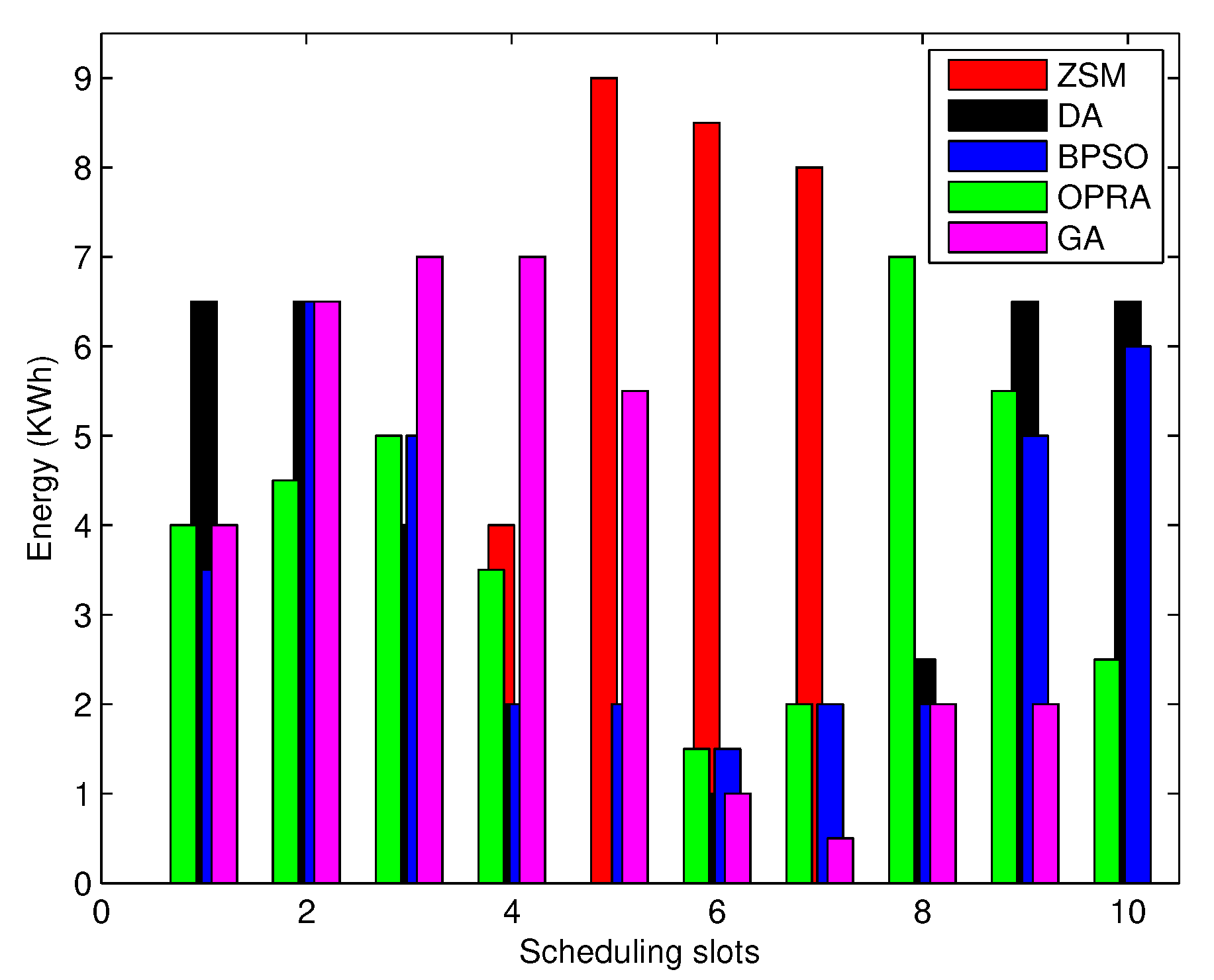
A novel DSEM model and EMC based on DA were proposed and implemented for the optimal energy management of residential user in this paper. The novel aspect of this work is the optimal selection of PV arrays and ESS, based on which the optimal load scheduling algorithms have been designed. Prior to this, we categorized the load into base, schedulable, semi-schedulable and critical according to user preferences and assigned predefined priorities in order to provide operation flexibility. Then, these loads were mathematically modelled in such a way that optimization algorithm can have better control. EMC is supported by optimum PV module selection and use scheme that efficiently shifts the high cost load from grid to an on-site PV and ESS. The cost reduction objective is achieved through optimal use of grid, PV and ESS sources, where PV units and ESS act as a “primary source” of energy during peak hours. The intuition behind our model is to address the optimal management of base, semi-schedulable, schedulable, and critical energy demands, time varying price signal, optimal selection and integration of PV modules, energy harvesting from PV modules and use of stored energy to maximize comfort level and minimize the end user electricity cost and PAR. Simulation results show that EMC based on DA achieved the maximum comfort level and also optimally scheduled the load, minimized the electricity cost and PAR in comparison with BPSO, OPRA and GA. An evaluation of the proposed algorithm in comparison with other algorithms is done based on an increased number of time slots and household loads and the presented results validates that the proposed algorithm leads to better solution. In addition, incorporating PV-based energy generation and storage system in the HEM architecture leads to better synergy between electricity consumption and PV production. The result is that the end user electricity cost is reduced by 52% and grid stability is increased by minimizing the PAR to 10.22% in comparison with ZSM. In future, we will update this model with other modules such as: (i) integration of windmill energy generation system, (ii) an energy exchange model among several micro smart grids, (iii) cloud-based infrastructure to connect micro smart grids, (iv) join the grid using Blockchain technology, (v) efficient storage system and (vi) facilitating electrical vehicles.

References

1. Albu, M.M.; Sănduleac, M.; Stănescu, C. Syncretic use of smart meters for power quality monitoring in emerging networks. IEEE Trans. Smart Grid 2016, 8, 485–492. [Google Scholar] [CrossRef]
2. Karimi, B.; Namboodiri, V.; Jadliwala, M. Scalable meter data collection in smart grids through message concatenation. IEEE Trans. Smart Grid 2015, 6, 1697–1706. [Google Scholar] [CrossRef]
3. Ye, F.; Qian, Y.; Hu, R.Q. A real-time information based demand-side management system in smart grid. IEEE Trans. Parallel Distrib. Syst. 2015, 27, 329–339. [Google Scholar] [CrossRef]
4. Viswanath, S.K.; Yuen, C.; Tushar, W.; Li, W.T.; Wen, C.K.; Hu, K.; Chen, C.; Liu, X. System design of the internet of things for residential smart grid. IEEE Wirel. Commun. 2016, 23, 90–98. [Google Scholar] [CrossRef] [Green Version]
5. Minoli, D.; Sohraby, K.; Occhiogrosso, B. IoT considerations, requirements, and architectures for smart buildings—Energy optimization and next-generation building management systems. IEEE Internet Things J. 2017, 4, 269–283. [Google Scholar] [CrossRef]
6. Forouzandehmehr, N.; Han, Z.; Zheng, R. Stochastic dynamic game between hydropower plant and thermal power plant in smart grid networks. IEEE Syst. J. 2014, 10, 88–96. [Google Scholar] [CrossRef]
7. Pahasa, J.; Ngamroo, I. Coordinated control of wind turbine blade pitch angle and PHEVs using MPCs for load frequency control of microgrid. IEEE Syst. J. 2014, 10, 97–105. [Google Scholar] [CrossRef]
8. Abdrabou, A. A wireless communication architecture for smart grid distribution networks. IEEE Syst. J. 2014, 10, 251–261. [Google Scholar] [CrossRef]
9. Shang, Y. Consensus of hybrid multi-agent systems with malicious nodes. IEEE Trans. Circuits Syst. II Express Briefs 2019. [Google Scholar] [CrossRef]
10. Eid, B.M.; Rahim, N.A.; Selvaraj, J.; El Khateb, A.H. Control methods and objectives for electronically coupled distributed energy resources in microgrids: A review. IEEE Syst. J. 2014, 10, 446–458. [Google Scholar] [CrossRef]
11. Kahrobaeian, A.; Mohamed, Y.A.R.I. Interactive distributed generation interface for flexible micro-grid operation in smart distribution systems. IEEE Trans. Sustain. Energy 2012, 3, 295–305. [Google Scholar] [CrossRef]
12. Kumar, S.; Lee, G.K.F.; Ozturk, Y. Residential and Commercial Energy Management System. U.S. Patent 13/660,876, 6 June 2013. [Google Scholar]
13. Muralitharan, K.; Sakthivel, R.; Shi, Y. Multiobjective optimization technique for demand side management with load balancing approach in smart grid. Neurocomputing 2016, 177, 110–119. [Google Scholar] [CrossRef]
14. Rahman, A.; Liu, X.; Kong, F. A survey on geographic load balancing based data center power management in the smart grid environment. IEEE Commun. Surv. Tutor. 2013, 16, 214–233. [Google Scholar] [CrossRef]
15. Hassan, N.; Pasha, M.; Yuen, C.; Huang, S.; Wang, X. Impact of scheduling flexibility on demand profile flatness and user inconvenience in residential smart grid system. Energies 2013, 6, 6608–6635. [Google Scholar] [CrossRef]
16. Zhang, S.; Liu, J.; Zhao, B.; Cao, J. Cloud computing-based analysis on residential electricity consumption behavior. Power Syst. Technol. 2013, 37, 1542–1546. [Google Scholar]
17. Li, H.; Lin, X.; Yang, H.; Liang, X.; Lu, R.; Shen, X. EPPDR: An efficient privacy-preserving demand response scheme with adaptive key evolution in smart grid. IEEE Trans. Parallel Distrib. Syst. 2013, 25, 2053–2064. [Google Scholar] [CrossRef] [Green Version]
18. Mohamed, M.A.; Eltamaly, A.M.; Farh, H.M.; Alolah, A.I. Energy management and renewable energy integration in smart grid system. In Proceedings of the 2015 IEEE International Conference on Smart Energy Grid Engineering (SEGE), Oshawa, ON, Canada, 17–19 August 2015; pp. 1–6. [Google Scholar]
19. Al-Aboosi, F.; El-Halwagi, M. An integrated approach to water-energy nexus in shale-gas production. Processes 2018, 6, 52. [Google Scholar] [CrossRef] [Green Version]
20. Tushar, W.; Chai, B.; Yuen, C.; Smith, D.B.; Wood, K.L.; Yang, Z.; Poor, H.V. Three-party energy management with distributed energy resources in smart grid. IEEE Trans. Ind. Electron. 2014, 62, 2487–2498. [Google Scholar] [CrossRef] [Green Version]
21. Chen, D.; Kalra, S.; Irwin, D.; Shenoy, P.; Albrecht, J. Preventing occupancy detection from smart meters. IEEE Trans. Smart Grid 2015, 6, 2426–2434. [Google Scholar] [CrossRef]
22. Gomez-Vilardebo, J.; Gündüz, D. Smart meter privacy for multiple users in the presence of an alternative energy source. IEEE Trans. Inf. Forensics Secur. 2014, 10, 132–141. [Google Scholar] [CrossRef] [Green Version]
23. Tan, O.; Gunduz, D.; Poor, H.V. Increasing smart meter privacy through energy harvesting and storage devices. IEEE J. Sel. Areas Commun. 2013, 31, 1331–1341. [Google Scholar] [CrossRef] [Green Version]
24. Rogers, J.; Averyt, K.; Clemmer, S.; Davis, M.; Flores-Lopez, F.; Frumhoff, P.; Kenney, D.; Macknick, J.; Madden, N.; Meldrum, J.; et al. Water-Smart Power: Strengthening the US Electricity System in a Warming World; Union of Concerned Scientists: Cambridge, MA, USA, 2013. [Google Scholar]
25. Averyt, K.; Macknick, J.; Rogers, J.; Madden, N.; Fisher, J.; Meldrum, J.; Newmark, R. Water use for electricity in the United States: An analysis of reported and calculated water use information for 2008. Environ. Res. Lett. 2013, 8, 015001. [Google Scholar] [CrossRef] [Green Version]
26. Kanyerere, T.; Tramberend, S.; Levine, A.D.; Mokoena, P.; Mensah, P.; Chingombe, W.; Goldin, J.; Fatima, S.; Prakash, M. Water futures and solutions: Options to enhance water security in sub-Saharan Africa. In Systems Analysis Approach for Complex Global Challenges; Springer: Cham, Switzerland, 2018; pp. 93–111. [Google Scholar]
27. Miceli, R. Energy management and smart grids. Energies 2013, 6, 2262–2290. [Google Scholar] [CrossRef] [Green Version]
28. Dodder, R.S.; Barnwell, J.T.; Yelverton, W.H. Scenarios for low carbon and low water electric power plant operations: Implications for upstream water use. Environ. Sci. Technol. 2016, 50, 11460–11470. [Google Scholar] [CrossRef] [PubMed]
29. Marler, R.T.; Arora, J.S. Survey of multi-objective optimization methods for engineering. Struct. Multidiscip. Optim. 2004, 26, 369–395. [Google Scholar] [CrossRef]
30. Das, I.; Dennis, J.E. A closer look at drawbacks of minimizing weighted sums of objectives for Pareto set generation in multicriteria optimization problems. Struct. Optim. 1997, 14, 63–69. [Google Scholar] [CrossRef] [Green Version]
31. Armstrong, N.R.; Shallcross, R.C.; Ogden, K.; Snyder, S.; Achilli, A.; Armstrong, E.L. Challenges and opportunities at the nexus of energy, water, and food: A perspective from the southwest United States. MRS Energy Sustain. 2018, 5. [Google Scholar] [CrossRef] [Green Version]
32. Javaid, N.; Ullah, I.; Akbar, M.; Iqbal, Z.; Khan, F.A.; Alrajeh, N.; Alabed, M.S. An intelligent load management system with renewable energy integration for smart homes. IEEE Access 2017, 5, 13587–13600. [Google Scholar] [CrossRef]
33. Clauser, C.; Ewert, M. The renewables cost challenge: Levelized cost of geothermal electric energy compared to other sources of primary energy–review and case study. Renew. Sustain. Energy Rev. 2018, 82, 3683–3693. [Google Scholar] [CrossRef]
34. Parra, D.; Norman, S.A.; Walker, G.S.; Gillott, M. Optimum community energy storage for renewable energy and demand load management. Appl. Energy 2017, 200, 358–369. [Google Scholar] [CrossRef]
35. Smith, J.C.; Milligan, M.R.; DeMeo, E.A.; Parsons, B. Utility wind integration and operating impact state of the art. IEEE Trans. Power Syst. 2007, 22, 900–908. [Google Scholar] [CrossRef]
36. Bird, L.; Milligan, M. Lessons from Large-Scale Renewable Energy Integration Studies; Technical Report; National Renewable Energy Lab. (NREL): Golden, CO, USA, 2012.
37. Brouwer, A.S.; Van Den Broek, M.; Seebregts, A.; Faaij, A. Impacts of large-scale Intermittent Renewable Energy Sources on electricity systems, and how these can be modeled. Renew. Sustain. Energy Rev. 2014, 33, 443–466. [Google Scholar] [CrossRef]
38. Wang, Y.; Lin, X.; Pedram, M. A near-optimal model-based control algorithm for households equipped with residential photovoltaic power generation and energy storage systems. IEEE Trans. Sustain. Energy 2015, 7, 77–86. [Google Scholar] [CrossRef]
39. Al Busaidi, A.S.; Kazem, H.A.; Al-Badi, A.H.; Khan, M.F. A review of optimum sizing of hybrid PV–Wind renewable energy systems in oman. Renew. Sustain. Energy Rev. 2016, 53, 185–193. [Google Scholar] [CrossRef]
40. Pereira, M.; Limon, D.; de la Peña, D.M.; Valverde, L.; Alamo, T. Periodic economic control of a nonisolated microgrid. IEEE Trans. Ind. Electron. 2015, 62, 5247–5255. [Google Scholar] [CrossRef]
41. Pereira, M.; de la Peña, D.M.; Limón, D. Robust economic model predictive control of a community micro-grid. Renew. Energy 2017, 100, 3–17. [Google Scholar] [CrossRef]
42. Zhang, X.; Bao, J.; Wang, R.; Zheng, C.; Skyllas-Kazacos, M. Dissipativity based distributed economic model predictive control for residential microgrids with renewable energy generation and battery energy storage. Renew. Energy 2017, 100, 18–34. [Google Scholar] [CrossRef]
43. Sechilariu, M.; Wang, B.; Locment, F. Building integrated photovoltaic system with energy storage and smart grid communication. IEEE Trans. Ind. Electron. 2012, 60, 1607–1618. [Google Scholar] [CrossRef]
44. Lee, C.K.; Hui, S.Y.R. Reduction of energy storage requirements in future smart grid using electric springs. IEEE Trans. Smart Grid 2013, 4, 1282–1288. [Google Scholar] [CrossRef]
45. Ding, Y.M.; Hong, S.H.; Li, X.H. A demand response energy management scheme for industrial facilities in smart grid. IEEE Trans. Ind. Inform. 2014, 10, 2257–2269. [Google Scholar] [CrossRef]
46. Borghetti, A.; D’Ambrosio, C.; Lodi, A.; Martello, S. An MILP approach for short-term hydro scheduling and unit commitment with head-dependent reservoir. IEEE Trans. Power Syst. 2008, 23, 1115–1124. [Google Scholar] [CrossRef] [Green Version]
47. Pham, T.H.; Wurtz, F.; Bacha, S. Optimal operation of a PV based multi-source system and energy management for household application. In Proceedings of the 2009 IEEE International Conference on Industrial Technology, Gippsland, Australia, 10–13 February 2009; pp. 1–5. [Google Scholar]
48. Lu, B.; Shahidehpour, M. Short-term scheduling of battery in a grid-connected PV/battery system. IEEE Trans. Power Syst. 2005, 20, 1053–1061. [Google Scholar] [CrossRef]
49. Rasheed, M.; Javaid, N.; Ahmad, A.; Jamil, M.; Khan, Z.; Qasim, U.; Alrajeh, N. Energy optimization in smart homes using customer preference and dynamic pricing. Energies 2016, 9, 593. [Google Scholar] [CrossRef] [Green Version]
50. Margaret, V.; Rao, K.U.; Ganeshprasad, G. Intelligent load shedding using ant colony algorithm in smart grid environment. In Power Electronics and Renewable Energy Systems; Springer: New Delhi, India, 2015; pp. 1149–1162. [Google Scholar]
51. Stoppato, A.; Cavazzini, G.; Ardizzon, G.; Rossetti, A. A PSO (particle swarm optimization)-based model for the optimal management of a small PV (Photovoltaic)-pump hydro energy storage in a rural dry area. Energy 2014, 76, 168–174. [Google Scholar] [CrossRef]
52. Marini, F.; Walczak, B. Particle swarm optimization (PSO). A tutorial. Chemom. Intell. Lab. Syst. 2015, 149, 153–165. [Google Scholar] [CrossRef]
53. Phuangpornpitak, N.; Tia, S. Opportunities and challenges of integrating renewable energy in smart grid system. Energy Procedia 2013, 34, 282–290. [Google Scholar] [CrossRef] [Green Version]
54. Samadi, P.; Mohsenian-Rad, H.; Schober, R.; Wong, V.W. Advanced demand side management for the future smart grid using mechanism design. IEEE Trans. Smart Grid 2012, 3, 1170–1180. [Google Scholar] [CrossRef]
55. Li, N.; Chen, L.; Low, S.H. Optimal demand response based on utility maximization in power networks. In Proceedings of the 2011 IEEE Power and Energy Society General Meeting, Detroit, MI, USA, 24–28 July 2011; pp. 1–8. [Google Scholar]
56. Basit, A.; Sidhu, G.A.S.; Mahmood, A.; Gao, F. Efficient and autonomous energy management techniques for the future smart homes. IEEE Trans. Smart Grid 2015, 8, 917–926. [Google Scholar] [CrossRef]
57. Erol-Kantarci, M.; Mouftah, H.T. Wireless sensor networks for cost-efficient residential energy management in the smart grid. IEEE Trans. Smart Grid 2011, 2, 314–325. [Google Scholar] [CrossRef]
58. Ma, J.; Chen, H.H.; Song, L.; Li, Y. Residential load scheduling in smart grid: A cost efficiency perspective. IEEE Trans. Smart Grid 2015, 7, 771–784. [Google Scholar] [CrossRef]
59. Saber, A.Y.; Venayagamoorthy, G.K. Resource scheduling under uncertainty in a smart grid with renewables and plug-in vehicles. IEEE Syst. J. 2011, 6, 103–109. [Google Scholar] [CrossRef]
60. Yang, J.S.; Choi, J.Y.; An, G.H.; Choi, Y.J.; Kim, M.H.; Won, D.J. Optimal scheduling and real-time state-of-charge management of energy storage system for frequency regulation. Energies 2016, 9, 1010. [Google Scholar] [CrossRef]
61. Javaid, N.; Ahmed, F.; Ullah, I.; Abid, S.; Abdul, W.; Alamri, A.; Almogren, A. Towards cost and comfort based hybrid optimization for residential load scheduling in a smart grid. Energies 2017, 10, 1546. [Google Scholar] [CrossRef] [Green Version]
62. Rasheed, M.B.; Javaid, N.; Malik, M.S.A.; Asif, M.; Hanif, M.K.; Chaudary, M.H. Intelligent multi-agent based multilayered control system for opportunistic load scheduling in smart buildings. IEEE Access 2019, 7, 23990–24006. [Google Scholar] [CrossRef]
63. Hung, D.Q.; Mithulananthan, N.; Lee, K.Y. Determining PV penetration for distribution systems with time-varying load models. IEEE Trans. Power Syst. 2014, 29, 3048–3057. [Google Scholar] [CrossRef]
64. Khatod, D.K.; Pant, V.; Sharma, J. Evolutionary programming based optimal placement of renewable distributed generators. IEEE Trans. Power Syst. 2012, 28, 683–695. [Google Scholar] [CrossRef]
65. Teng, J.H.; Luan, S.W.; Lee, D.J.; Huang, Y.Q. Optimal charging/discharging scheduling of battery storage systems for distribution systems interconnected with sizeable PV generation systems. IEEE Trans. Power Syst. 2012, 28, 1425–1433. [Google Scholar] [CrossRef]
66. Salameh, Z.M.; Borowy, B.S.; Amin, A.R. Photovoltaic module-site matching based on the capacity factors. IEEE Trans. Energy Convers. 1995, 10, 326–332. [Google Scholar] [CrossRef]
67. Joo, I.Y.; Choi, D.H. Distributed optimization framework for energy management of multiple smart homes with distributed energy resources. IEEE Access 2017, 5, 15551–15560. [Google Scholar] [CrossRef]
68. Paul, S.; Padhy, N.P. Resilient Scheduling Portfolio of Residential Devices and Plug-in Electric Vehicle by Minimizing Conditional Value at Risk. IEEE Trans. Ind. Inform. 2018, 15, 1566–1578. [Google Scholar] [CrossRef]
69. Jordehi, A.R. Binary particle swarm optimisation with quadratic transfer function: A new binary optimisation algorithm for optimal scheduling of appliances in smart homes. Appl. Soft Comput. 2019, 78, 465–480. [Google Scholar] [CrossRef]
70. Ma, K.; Hu, S.; Yang, J.; Xu, X.; Guan, X. Appliances scheduling via cooperative multi-swarm PSO under day-ahead prices and photovoltaic generation. Appl. Soft Comput. 2018, 62, 504–513. [Google Scholar] [CrossRef]
71. Hossain, E.; Khan, I.; Un-Noor, F.; Sikander, S.S.; Sunny, M.S.H. Application of Big Data and Machine Learning in Smart Grid, and Associated Security Concerns: A Review. IEEE Access 2019, 7, 13960–13988. [Google Scholar] [CrossRef]
72. Zhao, Z.; Lee, W.C.; Shin, Y.; Song, K.B. An optimal power scheduling method for demand response in home energy management system. IEEE Trans. Smart Grid 2013, 4, 1391–1400. [Google Scholar] [CrossRef]
73. Javaid, N.; Javaid, S.; Abdul, W.; Ahmed, I.; Almogren, A.; Alamri, A.; Niaz, I. A hybrid genetic wind driven heuristic optimization algorithm for demand side management in smart grid. Energies 2017, 10, 319. [Google Scholar] [CrossRef] [Green Version]
74. Iqbal, M.M.; Sajjad, I.A.; Amin, S.; Haroon, S.S.; Liaqat, R.; Khan, M.F.N.; Waseem, M.; Shah, M.A. Optimal Scheduling of Residential Home Appliances by Considering Energy Storage and Stochastically Modelled Photovoltaics in a Grid Exchange Environment Using Hybrid Grey Wolf Genetic Algorithm Optimizer. Appl. Sci. 2019, 9, 5226. [Google Scholar] [CrossRef] [Green Version]
Figure 1. DSEM Architecture.
Sustainability 12 00184 g001
Figure 2. Input set by the user.
Sustainability 12 00184 g002
Figure 3. EMC Load Management and Control Architecture.
Sustainability 12 00184 g003
Figure 4. A conceptual diagram of proposed hybrid energy system.
Sustainability 12 00184 g004
Figure 5. Schematic diagram showing the selecting of optimal load patterns using OPRA algorithm.
Sustainability 12 00184 g005
Figure 6. Generation of new off-springs from parent chromosomes through crossover operation.
Sustainability 12 00184 g006
Figure 7. Single point mutation.
Sustainability 12 00184 g007
Figure 8. Feasible region of Energy consumption.
Sustainability 12 00184 g008
Figure 9. RTP scheme obtained from a day-ahead electricity market.
Sustainability 12 00184 g009
Figure 10. User comfort profiles of different loads over the given time period.
Sustainability 12 00184 g010
Figure 11. Energy Consumption profiles using different optimization techniques over the given scheduling time period.
Sustainability 12 00184 g011
Figure 12. Solar irradiance and ambient temperature profiles over the period of 24 h.
Sustainability 12 00184 g012
Figure 13. Energy consumption profile against different optimization techniques with the integration of ESS.
Sustainability 12 00184 g013
Figure 14. Total cost incurred over the given time period using different optimization algorithms.
Sustainability 12 00184 g014
Figure 15. A comparison between energy consumption cost and total number of time slots against optimization algorithms (i.e., scalability w.r.t number of time slots).
Sustainability 12 00184 g015
Figure 16. A comparison between energy consumption cost and total number of time slots against optimization algorithms (i.e., scalability w.r.t number of time loads).
Sustainability 12 00184 g016
Figure 17. A comparison between computation time and total time slots.
Sustainability 12 00184 g017
Figure 18. A comparison between computation time and total number of loads.
Sustainability 12 00184 g018
Figure 19. PAR profiles of different algorithms over the period of one week.
Sustainability 12 00184 g019