A National Study on Transportation Affordability of HUD Housing Assistance Programs

Abstract

This national study is an effort to measure transportation costs and affordability for the major Housing and Urban Development (HUD) housing assistance programs since the transportation costs are the second largest expense of American households. This study estimates transportation costs for 76,000 address level properties from seven major HUD-designated affordable housing programs. Our transportation cost models are tailored for low-income households and account for built environmental determinants of travel, known as D variables, at the disaggregated level. We found that more than 44% of these properties in 326 U.S. metropolitan areas are unaffordable in terms of transportation costs. That could result in a waste of over $37.9 billion HUD spends annually to run these programs and subsidize housing for low-income families while some of these families spend substantial amount of their income on transportation. Our findings suggest that the provision of subsidized housing in mixed use, and transit-served neighborhoods would help low-income households to reduce their transportation costs even in auto-oriented sprawling regions. This study concludes with policy recommendations to local and federal governments and transit agencies on ways to incorporate transportation parameters to ensure true affordability for low-income residents of subsidized housing.

1. Introduction

The U.S. Department of Housing and Urban Development’s (HUD) simple ratio of income-to-housing costs to define housing affordability disregards other costs of living such as transportation [1] while transportation is the second largest expenditure category for a typical American household.

HUD’s rental assistance programs help more than 4.7 million low-income families pay their rent and HUD spent over $37.9 billion to run these programs and subsidize housing for these families. Consideration of housing costs only to measure affordability would result in low-income households living in subsidized housing to spend a substantial amount of their income on transportation, in some cases higher than their housing costs [2].

A recent national study by Hamidi et al. [2] found that 44% of households supported by Multifamily Section 8 program spend more than 15% of their income on transportation, and hence, those properties are unaffordable. While this study has shed a light on an overlooked but critical topic of transportation affordability for subsidized housing, the Multifamily Section 8 program is only one of several major HUD-subsidized housing programs and it is currently only limited to the renewal of existing contracts. There is still little evidence on transportation affordability and location efficiency of other major HUD-subsidized housing programs such as low-income housing tax credits (LIHTC), Public Housing and HOME Investment Partnership among others.

This national study seeks to investigate whether and to what extent the HUD-assisted major housing programs are affordable in terms of transportation costs in 326 Metropolitan Statistical Areas (MSAs) in the U.S. This study estimates transportation costs and affordability for nearly 76,000 HUD-subsidized properties by using transportation models that are tailored for low-income households and by measuring the built environmental determinants of travel, known as D variables, at the disaggregated address level for these properties. One major contribution of this study is to make comparisons across HUD programs in terms of transportation affordability. Finally, this study reviews the eligibility criteria and operation mechanisms of these programs and provides further discussions on incorporating transportation affordability as a key decision-making factor in these HUD-subsidized housing programs. Our findings would help federal and local housing authorities to make more location efficient investments.

2. Literature Review

2.1. Location Efficiency and Transportation Costs

The concept of location affordability infers to the inclusion of transportation costs, as a consequence of location choices, in housing affordability [3]. Location-efficient places are characterized by high accessibility to services and employment. As a result, location-efficient places support residents to drive less either by making a reduced number of trips due to opportunities for trip chaining or by modal shifts to walking, biking or transit [4,5]. Studies found such places are beneficial particularly for low-income households for several reasons. Living in more accessible places gives low-income households the ability to reduce their costs of driving and potentially increases household savings [6]. In other words, for those who cannot afford to maintain or drive a car, the presence of other options of transportation, such as walking, biking, or transit, is essential [7].

In recent years, studies have put emphasis on moving from solely looking into housing affordability to location affordability through integrating transportation costs into housing affordability [2,8]. At the national level, two major efforts were done by the Center for Neighborhood Technology (CNT) in 2006 (H + T index) and, more recently, HUD and the US Department of Transportation in 2013 (Location Affordability Index (LAI)) to create indices that measure location affordability as a combination of both housing and transportation costs for all census block groups in the U.S. These indices have been widely used by scholars and practitioners, but also have received criticism. One significant limitation of both H+T and LAI is that their transportation models are developed for a typical household not for low-income households, who are the primary users of HUD housing programs. Travel patterns and residential preferences of low-income households are substantially different from middle-income households [2].

Low-income households are primary users of HUD-subsidized housing. Recent studies have paid due attention to the importance of location for true affordability of subsidized housing. A national study by Koschinsky and Talen [9], for instance, found that only 23% of Housing Choice Voucher (HCV), Project-Based Rental Assistance, and public housing programs are located in walkable places based on Walkscore data. Similarly, Adkins et al. [7] studied the location efficiency of LIHTC program at the census block group (CBG) level in the U.S. They determined whether the LIHTC properties, measured in terms of the number of LIHTC units in CBGs, are accessible based on seven criteria including, residential density, road density, retail availability, regional auto accessibility, transit ridership, distance to rail transit, and transportation costs. They concluded that only 33% LIHTC properties are located in location efficient CBGs. While this is one of few studies at the national level with the focus on location efficiency of HUD-subsidized programs, the level of aggregation does not allow the analysis to account for the variations in socio-demographic and built environments within the same block group [10].

Addressing these gaps, Hamidi et al. [8] most recently employed a more rigorous methodology using address level disaggregate data to investigate the performance of HUD-subsidized units supported by eight different programs in the Dallas Fort Worth (DFW) region. They used the transportation costs model developed for low-income households who are eligible to receive assistance from HUD. Their models controlled for the availability of jobs within 10 minutes driving distance, transit frequency, land use mix, intersection density, employment, and population density within quarter-mile and half-mile network buffers around each property. These allowed the transportation cost models to precisely capture the built environment determinants of travel. Hamidi et al. [8] found a noticeable variation across programs and in different DFW cities in terms of transportation affordability citing LIHTC properties as the most affordable and Continuum of Care and Section 202 properties as the least affordable properties.

While this study contributes to a better understanding of transportation affordability across different HUD programs in DFW, it is not generalizable to other cities and metropolitan areas in the U.S. The DFW metro area is quite special in terms of car dependency and its sprawling patterns of development. Public transit is also not available in most parts of the region except the cities of Dallas and Fort Worth.

Our study seeks to provide a national investigation of transportation affordability for seven major HUD programs in the U.S. We use the address level disaggregated data of housing location and estimate transportation costs for these properties based on the built environmental features around them. Our findings provide policy guidelines on how to incorporate transportation efficiency as a key factor in various HUD programs in order to provide true affordability for the low-income population.

2.2. Major HUD Housing Programs and Location Efficiency Considerations

HUD provides housing assistance to low-income people through several programs and different programs have different mechanisms [11]. HUD’s housing acts and Code of Federal Regulations (CFR) are listed under Title 24, where various regulations are mentioned ranging from project design to nondiscrimination in the programs and activities [12,13]. The regulations related to location and neighborhood standards for programs such as public housing, project-based rental assistance (PBRA), HOME investment partnerships and programs for special groups (Section 202 and 811) are listed under pertinent sections of subtitle A or subtitle B of Title 24. For the LIHTC program, the statute for location criteria is stated under Section 42 of the Internal Revenue Code [14]. The location-related guidelines mentioned under different acts for particular programs have been summarized in

Table 1. Programs and transportation regulations.

Program Name	Code or Law	Guidelines Related to Location and Access to Facilities
Public Housing	Title 24 CFR § 941.202: Site and neighborhood standards	⮚ The housing must be accessible to educational, commercial social, recreational, health facilities, and other amenity facilities that are typically found in neighborhoods consisting largely of similar unassisted standard housing. ⮚ Travel time and costs via public transportation as well as private vehicles must not be excessive while commuting from neighborhoods to places of employment that have a range of jobs for low-income workers [15].
HOME investment partnership	Title 24 CFR § 983.57 Site selection standards	Same as above
Section 8 Project-Based Rental Assistance (PBRA)	Title 24 CFR § 983.57 Site selection standards [16]	Same as above
Rent Supplement	Title 24 CFR § 983.57 Site selection standards [16,17]	Same as above
Section 811 Supportive Housing for Persons with Disabilities	Title 24 CFR § 891.125 and additional regulations from CFR § 891.320 apply	Same as above and additional requirements of CFR § 891.320 apply: ⮚ The housing units under this program need to be located in neighborhoods where other family housing is also located. It may not be located adjacent to facilities like daycare centers for persons with disabilities, medical facilities or other types of housing facilities that are serving persons with disabilities [18]
Section 202 Supportive Housing for the Elderly	Title 24 CFR § 891.130 and Title 24 CFR 891.125. Site and neighborhood standards	⮚ Emphasize on the accessibility of sites to the commercial, social, educational, recreational, health, and civic facilities and services that are usually found in neighborhoods with unassisted standard housings [19,20]
Low-Income Housing Tax Credit	Section 42 of the Internal Revenue Code	⮚ If LIHTC assisted building is located in a qualified census tract (QCT) and household living in that building have income less than 60% AMI, then the household is eligible to receive services (daycare, outpatient clinical health care, career counseling, literacy training, education, and recreation) at free of charge or with an affordable fee in that building [21,22] (Section 42. Low-Income Housing Credit, N.D. a, b)

Note: Rent Supplement properties have the option to convert to long-term Project-Based Rental Assistance (PBRA) contracts via Rental Assistance Demonstration (RAD) [23]. Thus considering, Rent Supplement can follow the Codes of PBRA such as Section 8 PBRA.

.

The site and neighborhood standards of public housing, PBRA, and HOME programs state the physical characteristics requirements of the location (such as parcel size, slope, etc.) as well as the availability of utilities including streets [15,20]. HUD guidelines also indicate that the location should be suitable to comply with the relevant provision of “Title VI of the Civil Rights Act of 1964, the Fair Housing Act, and Rehabilitation Act of 1973” to prohibit discrimination in terms of race, color, religion, age, gender, disability or national origin [15,19,20].

Moreover, the site must have a broad range of housing choices to avoid excessive concentration of assisted households within an area that contains a higher proportion of low-income people [14,15,24]. For programs like Section 202 and Section 811, the sites for new housing units should not be in areas of ‘minority elderly concentration’ and must not be located in areas of racial mix in order to avoid increased ‘proportion of minority to nonminority elderly residents’. There could be some exceptions to this case in such areas if there are increasing housing needs that can be supported by new projects [15]. For all cases, the housing units must not be located in areas of detrimental conditions that can be harmful to dwellers and must be free from all natural or manmade hazards [15,20].

For the LIHTC program, development is encouraged in qualified census tracts (QCT) and difficult development areas (DDA) by providing incentives to the developers. The QCTs are the tracts where the poverty rate is above 25% or at least fifty percent households of that census tract have an income of less than 60% of area median income (AMI) [14,25]. The DDAs are areas where construction, development, and utility costs are high relative to AMI [14]. Although both DDA and QAP definitions concentrate on distressed areas in general, states and local housing authorities can set priorities and specify criteria for their own QAPs to distribute the tax credits [26]. For instance, the state QAPs can consider LIHTC projects to be located in areas proximity to daily destinations and other important services [7]. A good example is the Pennsylvania Housing Finance Agency that revised the LIHTC tax incentive criteria to prioritize developers who plan to develop their units within half-mile of fixed-route transit stops and in areas with a higher Walkscore [27]. Other state agencies have adopted different approaches to incorporate the transit requirements in their QAPs such as the presence of bus or rail stations within 0.1 to 5 miles of the development [28] Studies found that state QAPs that prioritize LIHTC projects with proximity to facilities and transit services are associated with higher location efficiency [7,28].

As all these above-mentioned programs have different codes or transportation regulations, it would be important to investigate how successful these programs are in providing location efficiency for their properties. To address this gap, we have conducted a national investigation of transportation affordability for about 76,000 address level disaggregated properties by incorporating transportation costs. We have followed the transportation cost models developed by Hamidi et al. [2] and controlled all specifications of their models to calculate the transportation affordability of HUD housing assistance recipients living in 326 regions in the U.S.

3. Methods

In our conceptual model, we considered the socio-demographic characteristics and D-Variables that have been extensively related to travel behavior [29]). The notion of D-Variable was first presented by Cervero and Kockelman [30] with three variables: Density, diversity, and design. Later, destination accessibility and distance to transit were included [31] Many peer-reviewed studies confirmed that these D variables significantly impact household travel behavior. These studies generally found that with the increase of development density, land use diversity, and street design the household’s vehicle miles traveled (VMT) decreases, on the other hand, with the increase of distance to transit the household VMT increases [32,33]. As the D variables influence the travel behavior and can influence the mode choice, hence they have been used as a determinant to calculate the transportation costs.

We follow the same methodology as Hamidi et al. [2] to measure D variables. Density, diversity, and design are measured within quarter-mile, half-mile, and one-mile buffers. Density is measured as two measures of population density and employment density, design is measured in terms of intersection density and street connectivity, diversity is measured in terms of job-population balance and land-use entropy (diversity index). Entropy indicates the balance between five different land uses, such as retail, educational, entertainment, health, and personal services. Entropy index ranges from 0 to 1, where 0 indicates all land is in single use to 1 where land is evenly used by different categories.

Destination accessibility is measured in terms of the percentage of regional jobs accessible within 10 minutes of travel time by automobile. Distance to transit is measured as the frequency of transit service within quarter-mile of the block group where the target property is located. Figure 1 shows the workflow with concise specifications as followed in this study.

We collected address level data from HUD portals for eight major programs for the year 2014. The programs included in this study are: Public Housing, Section 8 Project-Based Rental Assistance, Section 202 Supportive Housing for the Elderly Program (S202 PRAC), Section 811 Supportive Housing for Persons with Disabilities (S811 PRAC), Rent Supplement, HOME Investment Partnership Program, Below Market Interest Rate Section 236 (S236/BMIR) and LIHTC. After geocoding the addresses, we only included the properties located in 326 metropolitan areas and metro division in the U.S. excluding Hawaii, Alaska, and Puerto Rico.

As shown in Figure 1, we calculated the D- variables for quarter-, half-, and one-mile network buffers using the road network from ESRI Business Analyst (BA). We derived a total of 21 built environment variables around each property accounting for 5 D variables. The computed D-variables include: Percentage of regional employment accessible within 10 min by automobile (emp10), job population density (actden), land use mix of retail, entertainment, health, education and personal services (entropy), intersection density (intden), percentage of four-way intersections (pct4wy) and with average transit frequency (trafreq) within a quarter-mile of the block group.

Finally, we used the National Household Travel Survey (NHTS) database to obtain sociodemographic characteristics of a typical low-income household that qualifies for receiving housing subsidize from HUD. From this dataset, we extracted a subsample of households with annual incomes of less than 50 percent of adjusted median income (AMI), i.e., based on eligibility criteria from HUD. We used the average sociodemographic of this subsample for defining our typical low-income household. In this way, our transportation models are constant in terms of socio-demographic variable and the transportation affordability outcomes are solely location-based.

3.1. Transportation Cost Components

In our study, we measured three cost components by considering the typical travel modes and related costs for low-income households. We calculated the annual costs of public transit use, costs of vehicle ownership and costs associated with driving.

3.2. Fixed Costs of Vehicle Ownership

The vehicle ownership cost is a fixed or capital cost of owning automobile(s) for a household. We computed this cost using the following equation:

Cost of vehicle ownership = Household car ownership × estimated number of vehicles owned by the household

*Household car ownership = exp [−0.11 + (0.06 × average household size) + (0.14 × number of employed household members) + (0.009 × average household income) + (0.30 × dummy for single family units) − (0.002× percentage of regional employment accessible within 10 min by automobile) − (0.006 × job population density/1000) − (0.14 × land use mix(entropy)) − (0.0009 × intersection density) −(0.001 × percentage of four-way intersections) − (0.003 × transit frequency)]

*The equations are borrowed from Hamidi et al. [2].

We used a car ownership costs calculator called the ‘True Cost to Own^® pricing (TCO^®)’ to get the average vehicle ownership costs. This calculator was developed by Edmunds Inc. By using the specifications for the vehicle make, model, year, and style, this pricing system can provide estimation for total five-year costs of purchasing or maintaining a vehicle [34]. We decided to consider the most commonly used vehicle model and make that are generally popular among low-income households. Therefore, based on the HUD low-income standard, we created a sample of low-income households from the NHTS database and identified the 15 most popular vehicles owned by the low-income household sample. This represents about more than 34 percent of vehicles owned by low-income households in the NHTS database. According to the NHTS database, low-income households tend to purchase older cars. We acquired the five-year average costs of car ownership for these 15 vehicles in each state for the earliest year (2009) reported by the TCO®. For the fixed cost components of vehicle ownership, we considered the fixed cost parameters of TCO®, such as any federal tax credit, depreciation, repairs insurance premiums, interest on taxes, and fees. Finally, to obtain the average vehicle costs for low-income households, we weighted the five-year average costs for the 15 most popular vehicles found from the NHTS database. For the cost elements, we made the inflation adjustment for the year 2014 and multiplied the output with the number of cars owned by a household, which have been determined using the above-mentioned equation.

3.3. Costs of Driving

Secondly, we measured the costs of driving in terms of vehicle miles traveled by low-income households and the associated fuel costs. Metropolitan-level average gasoline prices were available for 2010 from the Oil Price Information Service (OPIS). We inflated them to 2014 dollars. The annual cost of driving is determined as:

Costs of VMT= fuel cost per mile × Household VMT per month

*Household VMT per month = Probability of a household having any VMT* Predicted VMT

(a)

Probability of a household having any VMT = EXP [1.72 + (0.23 × average household size) + (0.32 × number of employed household members) + (0.03 × average household income) + (0.85 × dummy for single family units) − (0.02 × percentage of regional employment accessible within 10 min by automobile) − (0.71 × land use mix(entropy)) − (0.003 × intersection density) − (0.01 × percentage of four-way intersections) − (0.0009 × transit frequency)]

(b)

Predicted VMT = exp [2.55 + (0.16 × average household size) + (0.18 × number of employed household members) + (0.007 × average household income) − (0.008 ×percentage of regional employment accessible within 10 min by automobile) − (0.005 × job population density/1000) − (0.29 × land use mix(entropy)) − (0.002 × intersection density) − (0.003 × percentage of four-way intersections) − (0.00009 × transit frequency)]

*The equations are borrowed from Hamidi et al. [2].

3.4. Costs of Transit Use

Thirdly, we computed households’ transit costs. The transit fare data is obtained from the National Transit Database. We computed average transit fare for each transit agency in the region by dividing the total transit revenue by the total number of unlinked passenger trips for the region.

Cost of transit use = Average transit fare per trip* Number of monthly household transit trips

*Number of monthly household transit trips = Probability of a household having any transit trip × Predicted number of transit trips

(a)

Probability of a household having any transit trip = EXP [−2.82 + (0.16 × average household size) + (0.27 × number of employed household members) − (0.02 × average household income) − (0.79 × dummy for single family units) + (0.48 × land use mix(entropy)) + (0.003 × intersection density) + (0.01 × percentage of four-way intersections) + (0.0009 × transit frequency)]

(b)

Predicted number of transit trips = EXP [0.85 + (0.16×average household size) − (0.006 × average household income) + (0.17 × land use mix (entropy)]

*The equations are borrowed from Hamidi et al. [2].

3.5. Total Transportation Costs and Affordability

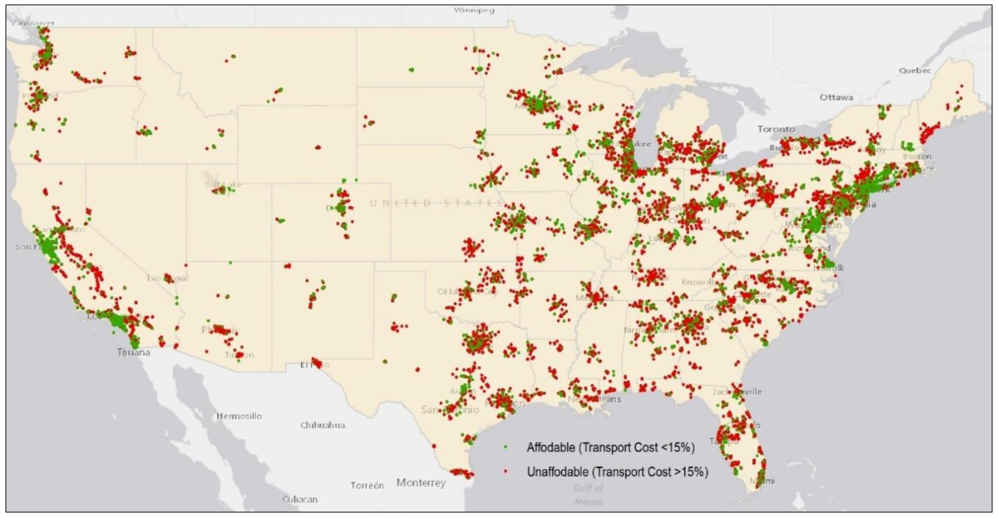
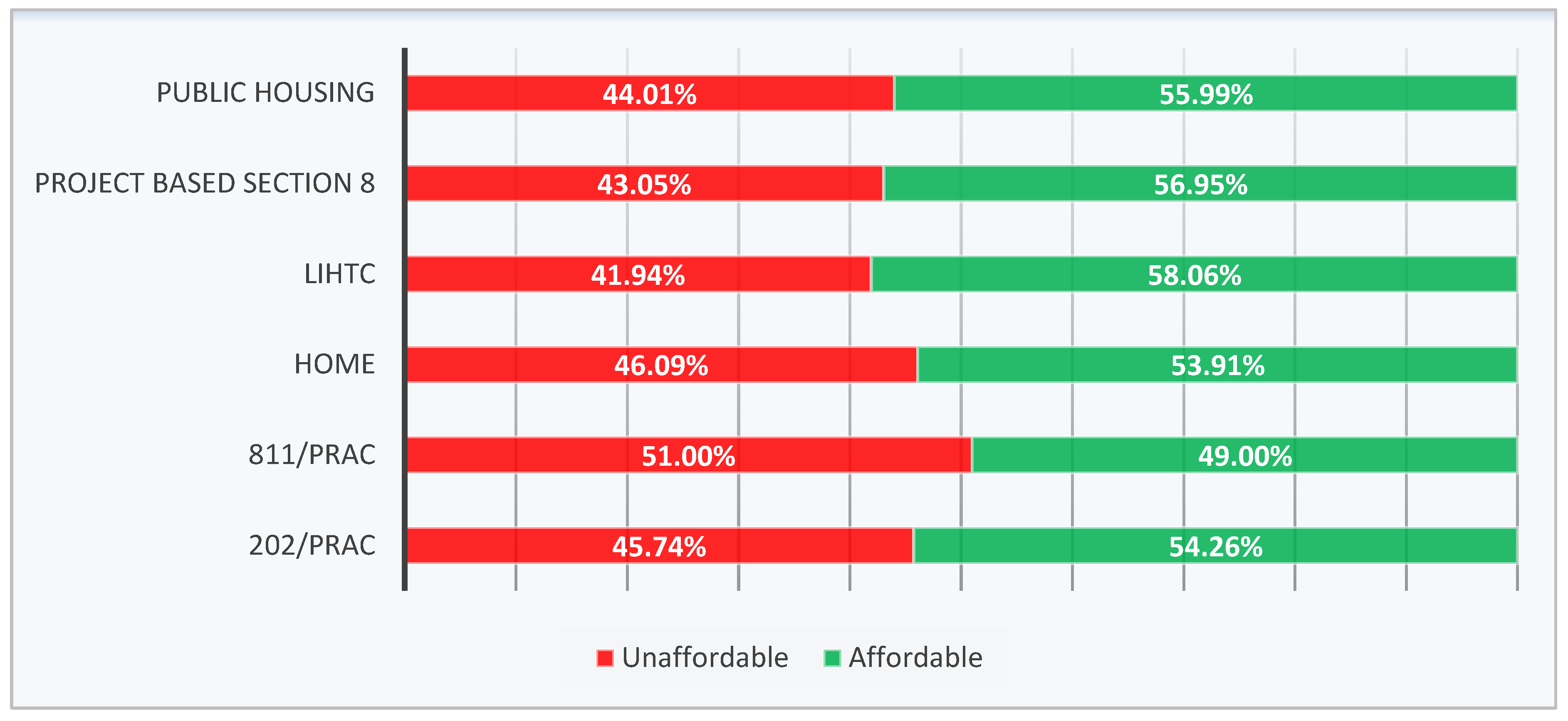
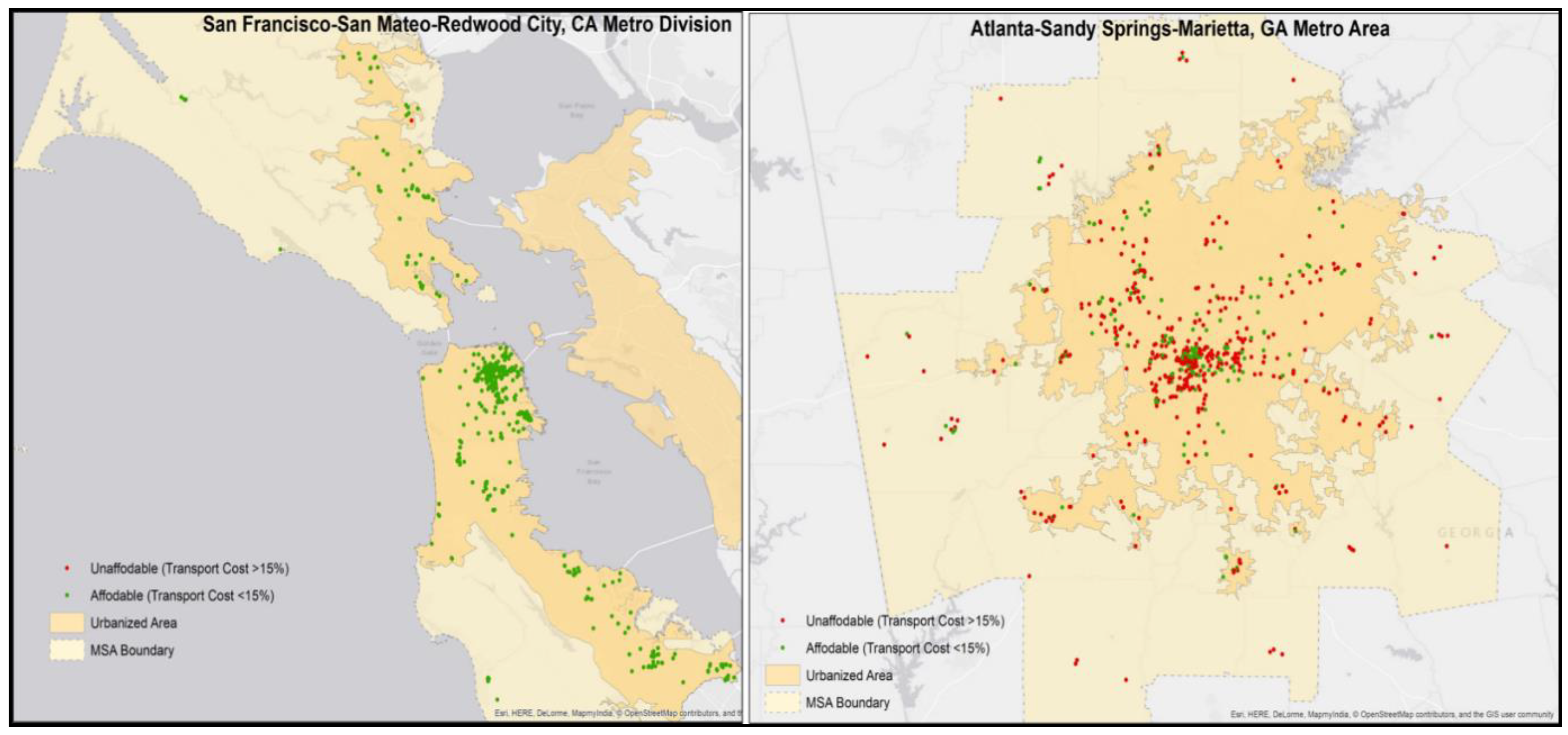
After calculating all the cost components for our model, we estimated total household transportation costs as the sum of three transportation cost components:

Total transportation costs = Costs of vehicle ownership + Costs of VMT + Costs of transit use

Finally, we computed the percentage of income spent on transportation for low-income households who are eligible to receive assistance from HUD based on the HUD income limits. According to HUD, less than 50% of Area Median Income (AMI) indicates very low income and less than 80% of AMI is low income [35]

Percentage of income spent on transportation = (Total transportation costs/Household income) × 100

If percentage of income spent on transportation ≤15%, (affordable = 1)

If percentage of income spent on transportation >15%, (unaffordable = 0)

4. Results

Figure 2 shows the distribution of affordable and unaffordable HUD-subsidized properties in terms of transportation costs in 326 U.S metropolitan areas. Our national analysis indicates that about 44% (33,626 properties out of 76,206 properties) HUD-assisted properties are unaffordable as they spend on average more than 15% of households’ income on transportation. The national average ratio of transportation costs to income for properties in our sample is 15.20%, which is very close to the 15% threshold suggested by CNT and HUD in H + T and LAI indices. As shown in Figure 2, metro areas with quality transit systems such as New York, NY or San Francisco, CA have a higher concentration of transport affordable properties than auto-oriented areas like Dallas, TX, Atlanta, GA or Orlando, FL.

Among 76,206 properties, we have the largest sample for the HOME program (30,691), and the second largest sample is for the LIHTC (26,309). Figure 3 presents the percentage of affordable properties in six different HUD programs in terms of transportation costs. More than 58% of the LIHTC properties (15,271 units) are affordable in terms of transportation which is the highest among all programs. On the other hand, the HOME program is providing about 54% of its properties in location efficient places. This percentage is the lowest (49%) for Section 811 program which was primarily designed to support persons with disabilities.

We also made a statistical comparison of the mean percentage of household income spent on transportation under different programs. The average income spent by all households of HOME properties is about 15.3% which is slightly higher than the affordability threshold, while a typical household who lives in LIHTC properties spend, an average, 15% of their income on transportation, precisely within the affordability threshold. The LIHTC found to be the most affordable, even in an auto-oriented region like the DFW metro area [8]. On the other hand, programs designed for people with special needs like Section 811 nationally spend on average 16% of their income on transportation and found to be the least transport affordable programs.

Table 2. Top ten large metropolitan areas with the lowest number of affordable properties in terms of transportation.

MSA Name	Affordability	Number of Affordable and Unaffordable Properties Under Different Programs								Total Properties	% Affordability	Sprawl Index
		PR202	PR811	HOME	LIHTC	PBS8	Pub Housing	RentSup	BMS236
Lakeland-Winter Haven, FL	Unaffordable	1	0	7	26	17	8		1	60	95.2	87.6
	Affordable	0	1	0	0	1	1		0	3	4.7
	Total	1	1	7	26	18	9		1	63
Poughkeepsie-Newburgh-Middletown, NY	Unaffordable	2	3	132	77	21	7	1	4	247	93.5	79.5
	Affordable	0	0	9	8	0	0	0	0	17	6.4
	Total	2	3	141	85	21	7	1	4	264
Chattanooga, TN-GA	Unaffordable	1	9	107	35	22	15		2	191	91.3	63.6
	Affordable	0	0	7	3	3	4		1	18	8.6
	Total	1	9	114	38	25	19		3	209
Wichita, KS	Unaffordable	10	8	55	86	37	11			207	88.8	91.7
	Affordable	1	0	4	15	6	0			26	11.2
	Total	11	8	59	101	43	11			233
Gary, IN	Unaffordable	2	8	55	51	22	18			156	88.1	96.7
	Affordable	2	1	7	5	5	1			21	11.9
	Total	4	9	62	56	27	19			177
Nashville-Davidson--Murfreesboro--Franklin, TN	Unaffordable	7	8	427	164	37	21			664	87.6	51.7
	Affordable	5	2	41	33	8	5			94	12.4
	Total	12	10	468	197	45	26			758
Memphis, TN-MS-AR	Unaffordable	5	5	237	158	48	37		1	491	84.4	70.8
	Affordable	6	2	29	33	18	3		0	91	15.6
	Total	11	7	266	191	66	40		1	582
Columbia, SC	Unaffordable	1	9	52	79	34	6		1	182	84.3	67.4
	Affordable	1	0	8	15	8	2		0	34	15.7
	Total	2	9	60	94	42	8		1	216
Toledo, OH	Unaffordable	9	15	147	91	47	6			315	83.1	100.9
	Affordable	1	4	37	13	8	1			64	16.9
	Total	10	19	184	104	55	7			379
Pittsburgh, PA	Unaffordable	28	31	263	185	185	101	1	3	797	82.0	95.4
	Affordable	6	5	66	45	29	24	0	0	175	18.0
	Total	34	36	329	230	214	125	1	3	972

Note: PR202 = Section 202 Supportive Housing for the Elderly Program; PR 811= Section 811 Supportive Housing for Persons with Disabilities; PBS8 = Project-Based Section 8; PubHouing = Public Housing; RentSup = Rent Supplement; BMS236= Section 236/BMIR, Composite Sprawl index for MSAs attained from https://gis.cancer.gov/tools/urban-sprawl/.

presents the top ten large regions (population of more than 0.5 million) with the highest number of unaffordable HUD-subsidized properties once accounting for transportation costs along with the sprawl index for each region [36,37]. The sprawl index value above 100 indicates more compactness, while the values below 100 indicate the sprawling region.

Almost all of the regions in Table 2 are among the most sprawling metro areas in the US. For example, in Pittsburg, PA, about 80% of all assisted properties are unaffordable in terms of transportation. Even though in Pennsylvania, state agencies have started to provide incentives to developers to invest in walkable and transit-served areas for programs like LIHTC, but it still is listed among the unaffordable MSAs. Of course, these changes in the program are relatively recent and it will take more time to see their impacts on the ground.

On the other side of the spectrum,

Table 3. Ten large metropolitan areas with the highest number of affordable properties in terms of transportation costs.

MSA Name	Affordability	Number of Affordable and Unaffordable Properties under Different Programs								Total Properties	% Affordability	Sprawl Index
		PR202	PR811	HOME	LIHTC	PBS8	Pub Housing	RentSup	BMS236
San Francisco-San Mateo-Redwood City, CA	Unaffordable	0	0	0	1	0	0	0	0	1	0.2	194.3
	Affordable	18	15	202	204	119	34	2	6	600	99.8
	Total	18	15	202	205	119	34	2	6	601
Bridgeport-Stamford-Norwalk, CT	Unaffordable	0	0	0	0	1	0		0	1	0.4	121.6
	Affordable	6	4	122	70	62	37		1	302	99.6
	Total	6	4	122	70	63	37		1	303
San Jose-Sunnyvale-Santa Clara, CA	Unaffordable	0	0	3	5	2	0	0	0	10	2.5	128.7
	Affordable	4	6	102	219	57	1	2	3	394	97.5
	Total	4	6	105	224	59	1	2	3	404
Oakland-Fremont-Hayward, CA	Unaffordable	0	0	4	15	3	1		0	23	3.3	127.2
	Affordable	29	16	187	304	104	34		4	678	96.7
	Total	29	16	191	319	107	35		4	701
New York-White Plains-Wayne, NY-NJ	Unaffordable	5	9	78	53	35	27	3	3	213	4.8	203.4
	Affordable	113	42	1179	2020	610	227	37	29	4257	95.2
	Total	118	51	1257	2073	645	254	40	32	4470
Santa Ana-Anaheim-Irvine, CA	Unaffordable		0	17	7	2				26	5.2	139.7
	Affordable		5	292	139	45				481	94.8
	Total		5	309	146	47				507
Washington-Arlington-Alexandria, DC-VA-MD-WV	Unaffordable	1	6	16	30	8	1	0	0	62	5.6	107.2
	Affordable	17	40	281	436	183	83	4	5	1049	94.4
	Total	18	46	297	466	191	84	4	5	1111
Los Angeles-Long Beach-Glendale, CA	Unaffordable	5	15	60	44	40	2	0	1	167	6.4	130.3
	Affordable	57	62	1028	828	457	27	1	9	2469	93.6
	Total	62	77	1088	872	497	29	1	10	2636
New Haven-Milford, CT	Unaffordable	0	1	6	9	10	5	1	0	32	6.9	116.3
	Affordable	12	9	216	72	70	48	0	2	429	93.1
	Total	12	10	222	81	80	53	1	2	461
Bethesda-Rockville-Frederick, MD	Unaffordable	1	4	18	3	2	0	1	0	29	8.9	114.7
	Affordable	2	29	107	89	42	21	3	4	297	91.1
	Total	3	33	125	92	44	21	4	4	326

Note: PR202 = Section 202 Supportive Housing for the Elderly Program; PR 811= Section 811 Supportive Housing for Persons with Disabilities; PBS8 = Project-Based Section 8; PbHou = Public Housing; RentSup = Rent Supplement; BMS236 = Section 236/BMIR, Composite Sprawl index for MSAs attained from https://gis.cancer.gov/tools/urban-sprawl/.

the top ten large regions (population of more than 0.5) with the highest number of affordable HUD-subsidized properties once accounting for transportation costs. Almost all MSAs listed in the table have a 90 to 100 percent affordability rate for LIHTC, HOME, Section 202, Section 811, and Public housing. In Bethesda-Rockville, MD the affordability rate for Section 202 (67%), Section 811 (88%), and HOME (86%) are lower than other major programs like LIHTC and public housing.

All HUD designated properties in San Francisco- San Mateo, CA, the region with one of the best transit system, dense, compact, and mixed-uses [36] are located in location efficient areas and are affordable in terms of transportation (as shown in Figure 4) while in Atlanta-Sandy Spring, GA (composite sprawl index of 41), almost 70% of HUD designated properties found to be unaffordable in terms of transportation costs (Figure 4). As indicated by literature, sprawl increases the travel distance, vehicle ownership and decreases the opportunities for commuting by transit, which, in turn, increases the overall household transportation costs [38,39,40] On the other hand, due to lower VMT and options for other active modes of travel, transportation costs can sharply decrease in compact areas [37].

However, this does not imply that transportation affordability could not be achieved in more sprawling regions, rather it is more important to carefully consider subsidizing the housing into location efficient places in sprawling regions. Of course, it will be a more difficult goal to achieve due to high correlation of sprawl with auto-dependency and the fact that more than 90% of transportation costs are driving-related expenses. The sprawling regions are also less transit-friendly which results in the lack of transportation options other than driving for residents. One way to achieve transportation affordability in sprawling regions is to designate subsidized housing units in places where the immediate neighborhood is walkable, accessible, mixed-use, and served by transit. Figure 5 shows an example of a location efficient property in Tulsa, OK MSAs (compactness index of 86.64). The typical low-income household, who lives in this property, spend about 12% of their budget on transportation. That property has access to a range of amenities with vibrant land use mix within half a mile network buffer. Transit availability with high frequency and increased street connectivity helps low-income households to have lower transportation costs.

On the other hand, even in most compact regions, a HUD-subsidized unit could be unaffordable in terms of transportation if it is located in a place that has little to no amenities available within the walkable distance and is not served by transit. Moreover, the cul-de-sac street patterns of the area decrease the street connectivity, which consequently increases the travel distance and eventually the transportation costs and decreases affordability.

Therefore, the surrounding built environment has a noticeable impact on the transportation affordability of low-income housing. It is vital for housing authorities both in the sprawling and compact regions to pay attention to the immediate surroundings of the neighborhood and also the availability of public transit to ensure the low-income people can live in truly affordable areas.

5. Discussions

Although different HUD programs have different guidelines for site selection and location considerations (see Table 1), the majority of these guidelines focus on issues related to discrimination and tend to discourage the concentration of poverty. Few of these guidelines, which focus on transportation, recommend that accessibility for the subsidized units under these programs should be at the level of similar unassisted standard housing. This is, first of all, a subjective criterion and it is hard to quantify, in a standard way, the level of accessibility for “similar unassisted standard housing”.

Secondly, the transportation needs of low-income households are different from other income groups. Low-income households are more likely to own few and older model cars that are not fuel-efficient, which translates into higher vehicle maintenance and fuel costs and, in turn, would result in substantially higher transportation costs. Low-income households are also more likely to take transit if it is available and convenient. One of the most widely cited location efficient type of development is transit-oriented developments (TOD). TODs are dense, walkable with a mix of housing, commercial and other buildings used in areas next to a transit station [41]. Planning for affordable housing in TODs involves the development of an integrated housing and transportation plan in coordination between cities, housing agencies, and transit providers. Cities can adopt policies that support the economic feasibility of affordable housing development in TOD sites.

There is a lack of objective for transportation-related requirements in site selection and funding allocation of almost all of the eight HUD programs covered in this study. The policies of the programs need to be revised by incorporating further specifications of transportation parameters which would ensure location efficiency and reduced transportation costs.

For example, as LIHTC developers are incentivized to develop their housing in QCTs and DDAs, the factors for determining the QCTs and DDAs could be revised. Access to amenities, transit, and other transportation components should be incorporated within QCT and DDA criteria. Though some states such as California, New Jersey, or Pennsylvania have already incorporated the LE criteria and proximity to transit in LIHTC program [27,28], a more unified and efficient approach is needed to incorporate LE at the federal level decision-making. Even though the LIHTC program is relatively doing better than the other seven HUD programs covered in this study, our findings show that there is still room to increase the location efficiency of this program in different regions.

While this study focused specifically on transportation affordability, there are potential tradeoffs of location efficiency characteristics and other qualities of the area. Some possible tradeoffs mentioned in affordable housing literature are school quality [42], congestion [43], neighborhood crime [44], pollution or environmental quality [43], poverty concentration and racial segregation [45]. Our study did not capture such tradeoffs due to data limitations at the national level, but again the focus of this study was not on the residential choice of low-income households, rather to measure the effectiveness of HUD programs in terms of transportation affordability. We recommend future studies to consider incorporating other locational factors, which could affect residential choices, to the concept of housing affordability.

In a number of cases, the provision of low-income housing in certain areas face oppositions due to the “Not in My Backyard” belief of surrounding neighbors [46] which is widely cited as a barrier for the success of such housing programs [47,48]. This gives rise to social segregation and spatial mismatch. As a result of such oppositions, properties may tend to locate farther from economically advantageous areas and would force low-income residents of subsidized housing to travel longer distances to access to facilities [49]. Future studies could take a deeper look into this issue and investigate policy approaches that facilitate planning for mix-income neighborhoods.

6. Conclusions and Implications

Our findings recommend housing authorities and practitioners to prioritize contract renewals as well as provide new developments in walkable, mixed land use and transit-served areas. In providing rental assistance under different programs, the programs should also consider the transportation costs to factor in while calculating the share of rent for a household. In addition, technical assistance, financial incentive, and training can be provided to the housing agencies to guide them about the importance of effective housing development in location efficient places. Before making decisions regarding the provision of affordable housing in a certain area, the local government, housing authorities, planners, practitioners, and policy-makers can use data, transportation cost estimates, and models of this study to determine location affordability.

As mentioned in the previous section, policies could be adopted to encourage planning for affordable housing in TODs. This could be done through financial incentives such as Tax Increment Financing or non-financial incentives such as parking reductions and density bonus permits. States could use federal tax credits as incentives to support the development of affordable housing in TOD sites, particularly through the low-income housing tax credits (LIHTC) program. The Pennsylvania Housing Finance Agency has been successfully implementing this policy [50]. Moreover, planners in local housing agencies overseeing project-based multifamily programs could prioritize the renewal of existing contracts or new contracts within the catchment areas of TODs. Planners and housing agencies could also provide higher incentives to the property owners participating in the Housing Choice Voucher Program, requiring them to offer reduced rents to low-income tenants in TOD areas. These policies should also focus on the mitigation of potential gentrification and displacement effects associated with TOD projects by providing mixed-income housing options near transit stations in TOD sites. Finally, transportation planners could prioritize areas with a concentration of affordable units when planning for expansion of transit networks and future TODs.

Other than TODs, the provision of assisted housing in areas with high accessibility to facilities can be incentivized by Government and city officials through controlling the urban land market. As land is scarce and development is expensive in high accessibility and central urban areas, it is important to promote better planning for the location of housing development and the distribution of daily activities within an accessible limit. Federal policies should help to reduce the regulatory barriers to support the housing market for such development. For this, housing and transportation policies should be considered or revised in an integrated way to reduce the cost burden for low-income families.

Finally, the local housing agencies could collaborate with transit agencies to prioritize areas with a high concentration of HUD-subsidized units in non-TOD areas, when planning for transit expansion, coverage, and frequency. To avoid transport-related social exclusion of low-income people living in HUD-assisted housing, it is important to have an accessibility planning of public transit that will be highly integrated with those housings and other basic facilities such as employment, healthcare, and education [51]. A public transport network model can help to identify the spatial gap between transit service areas and low-income areas that need access to transit and other social needs [52,53]. This can help to improve the accessibility loss and address the nondiscriminatory dimension of transportation [54] Another alternative is to provide subsidized units in unaffordable locations with a transportation allowance that can compensate households for higher transportation costs. Such initiatives can ensure transportation equity.

References

1. Jewkes, M.D.; Delgadillo, L.M. Weaknesses of Housing Affordability Indices Used by Practitioners. J. Financ. Couns. Plan. 2010, 21, 43–52. [Google Scholar]
2. Hamidi, S.; Ewing, R.; Renne, J. How affordable is HUD affordable housing? Hous. Policy Debate 2016, 26, 437–455. [Google Scholar] [CrossRef] [Green Version]
3. The United States Environmental Protection Agency (EPA). Location Efficiency and Housing Type. 2011. Available online: http://www.epa.gov/sites/production/files/2014-03/documents/location_efficiency_btu.pdf (accessed on 28 May 2018).
4. Newmark, G.L.; Haas, P.M.; Pappas, J.; Schwartz, M.; Kenyon, A.; Unit, M.O. Income, location efficiency, and VMT: Affordable Housing as a Climate Strategy. Center for Neighborhood Technology Working Paper, Produced for the California Housing Partnership. 2015. Available online: https://chpc.net/wp-content/uploads/2016/05/CNT-Working-Paper-revised-2015-12-18.pdf (accessed on 20 July 2018).
5. Litman, T. Transportation Affordability: Evaluation and Improvement Strategies. Victoria Transport Policy Institute. 2017. Available online: http://www.vtpi.org/affordability.pdf (accessed on 28 July 2018).
6. Hartell, A.M. Evaluating the Concept of Location Affordability: Recent Data on the Relationship between Transportation, Housing, and Urban Form. Hous. Policy Debate 2017, 27, 356–371. [Google Scholar] [CrossRef]
7. Adkins, A.; Sanderford, A.; Pivo, G. How Location Efficient Is LIHTC? Measuring and Explaining State-Level Achievement. Hous. Policy Debate 2017, 27, 335–355. [Google Scholar] [CrossRef]
8. Hamidi, S.; Jahan, J.; Moazzeni, S. Does Location Matter? Performance Analysis of the Affordable Housing Programs with Respect to Transportation Affordability in Dallas Fort Worth (DFW) Metropolis. Transp. Res. Rec. 2018. [Google Scholar] [CrossRef]
9. Koschinsky, J.; Talen, E. Location Efficiency and Affordability: A National Analysis of Walkable Access and HUD-Assisted Housing. Hous. Policy Debate 2016, 26, 835–863. [Google Scholar] [CrossRef]
10. Guerra, E.; Kirschen, M. Housing Plus Transportation Affordability Indices: Uses, Opportunities, and Challenges. International Transport Forum Discussion Paper. 2016. Available online: https://www.itf-oecd.org/sites/default/files/docs/housing-transport-affordability.pdf (accessed on 22 July 2018).