1. Introduction
Ventilation of homes is necessary to maintain healthy and safe indoor air quality for the occupants. Most homes are ventilated with infiltration of air through small cracks and openings in the building shell structure and natural ventilation practices (opening windows and doors). Introduction of outdoor air is often needed to help dilute indoor air contaminants emitted from various indoor sources, and ventilation results in their removal from the indoor environment. Lower ventilation rates may result in elevated exposures from the accumulation of pollutants generated indoors and cause adverse health effects, such as exacerbation of asthma symptoms and other respiratory diseases, and sick building syndrome symptoms [
1,
2,
3,
4,
5,
6]. The American Society for Heating, Refrigerating, and Air-Conditioning Engineers (ASHRAE) 62.2 Standard provides guidelines for achieving ventilation and acceptable indoor air quality in residences and adding continuous mechanical ventilation in homes with insufficient natural ventilation [
7]. Home ventilation rates can be affected by many factors, one of them being retrofits made to the building shell.
In many locations, current home building practices are changing to build tighter homes and install mechanical ventilation that is energy efficient, such as using energy-recovery ventilators to save on energy losses and expenditures [
8,
9]. In existing buildings, energy-efficiency retrofits (EERs) must be applied to make buildings more energy-efficient. Such upgrades are often performed during the weatherization process by contractors and homeowners. In addition to the wide variety of energy upgrade activities done to building systems and appliances, EERs also focus on building envelope air-sealing techniques aimed to reduce infiltration and, consequentially, the consumption of energy needed for indoor temperature control. The air-sealing activities related to EERs include door and window weather-stripping, caulking of door and window frames, foam sealing of cracks in the building envelope, improving or adding insulation to walls, caulking around plumbing, and electrical and combustion appliance exhaust conduit penetrations through roofs and walls, including insulating around chimneys, and sealing of leakage points in the heating system ductwork [
10,
11]. Residential building EER programs in the US are subsidized through the US Department of Energy (DOE)’s Weatherization Assistance Program (WAP) since 1976 to increase energy savings in low-income communities. The DOE provides weatherization services to approximately 35,000 homes every year—a total of seven million homes were weatherized through the spring of 2018. DOE reports that weatherized single-family households experience an average of
$283 or more in annual energy savings [
10]. In addition to WAP, there are local and state entities that also provide energy-efficiency testing and retrofits in many communities.
While the aim of reduced energy consumption via home EER interventions may be well intentioned, the air-sealing activities can introduce a suite of indoor environmental quality (IEQ) problems, especially if adequate ventilation is impeded by the retrofits. The characteristics of a typical home are inter-related, such that changing one component directly or indirectly changes the operation of other components as well, which can influence indoor air pollutant exposures in the home. Tighter homes more readily depressurize when exhaust equipment is operated, making combustion appliances more prone to backdraft or spillage [
12]. Tighter buildings are also associated with elevated indoor radon concentrations [
13], in addition to moisture problems [
14,
15]. The US Environmental Protection Agency developed a protocol for guiding professional home energy upgrades while maintaining healthy IEQ for the occupants [
16]. However, the variability remains wide in the quality of energy retrofitting services provided by weatherization contractors [
17], which in turn affects indoor air quality in the retrofitted homes.
Previous studies investigated the impacts of EERs on IEQ [
18,
19,
20]. Energy retrofits can alter exposures to some indoor pollutants, and the use of new building materials can introduce a wide variety of toxic chemicals indoors following the retrofits [
20,
21,
22]. In studies of occupant satisfaction with the IEQ in green buildings, some report that occupants are more satisfied, while others report the opposite [
18]. A study of 514 homes across the US with indoor air contaminant measurements pre- and post-weatherization by the DOE’s WAP concluded that weatherization caused a small but statistically significant increase in radon and humidity, dependent on season [
20]. Another study, conducted in Ireland in 15 three-bedroom semi-detached cooperative social dwellings before and after energy upgrades, reported a significant increase in indoor concentrations of carbon dioxide, total volatile organic compounds (TVOC), and particulate matter smaller than 2.5 microns (PM
2.5) [
23]. Similarly, a study conducted in North Carolina in nine homes also found that homes had above-recommended levels of TVOC and formaldehyde after weatherization [
24]. EERs can also affect the rates of infiltration of outdoor air pollutants into the indoor environment. Past studies showed that changes in the infiltration of outdoor air pollutants with ventilation into the indoor built environment can have a significant impact on indoor air quality [
25,
26,
27,
28,
29]. The PTEAM study conducted in Riverside, California concluded that more than half of the indoor particles came from outdoors [
30]. On the other hand, some studies also identified that indoor sources contribute to the elevation of indoor particulate matter concentrations to many times the background indoor levels [
31,
32]. It is unclear from the existing literature if tighter buildings experience further exacerbation of indoor pollutant concentrations in low-income dwellings in urban areas, and how indoor air pollutant concentrations are affected in the long term by EER activities in these dwellings.
Investigation of the effects of EERs on the healthiness of the indoor environments of homes can be difficult and expensive to perform, especially if the sample size of the study is large enough to establish greater statistical confidence in the results. Hence, indirect assessment tools can be used for such investigations, such as noting various indicators that can be observed from the living spaces. In past studies, problems related to home characteristics, noted with observations and surveys, were associated with adverse health including asthma and depression [
33,
34,
35,
36]. A study of 1343 households in England and Scotland found that children living in better-quality housing generally experienced lower overall mortality rates as adults. Housing characteristics were qualified during a home visit, and observations were recorded on crowding, water supply, cleanliness of home, and adequacy of ventilation. Note that these data were from the 1930s and in the UK; the housing conditions today in the US are quite different. The European Community Health Respiratory Survey showed that indoor mold growth in homes had an adverse health effect on adult asthma [
37]. A US study of over 15,000 children reported home dampness (water damage, mold) was associated with significantly increased respiratory symptoms [
38]. Studies of house dust focused on the presence of dust mites, bacteria, fungi, and their relationship to housing characteristics and respiratory health [
39,
40,
41], and also on lead-contaminated house dust [
42]. Some studies tried quantifying the home healthiness based on the perceived indoor environmental quality (PIEQ). Studies investigated the occupants’ perception of stuffiness, dryness, coldness, draftiness, and sufficiency of ventilation and compared symptoms and PIEQ in homes with different ventilation systems; the authors concluded that the occupants of buildings with natural ventilation had more symptoms and/or complaints than with mechanical ventilation [
43,
44]. In a study of offices, natural ventilation improved overall satisfaction with the working environment compared to air conditioning in buildings [
45]. PIEQ was also used in past studies as a significant subjective indicator of thermal comfort and indoor air quality and symptoms of sick building syndrome [
46,
47,
48]. A thorough review of human thermal comfort in buildings points out that there are many factors that influence the perception of comfort in the indoor environment including culture, age, gender, space, layout, etc. [
49].
While most studies on IEQ impacts of EERs focus on indoor concentrations of specific pollutants, there are limited data on how the air-sealing activities affect building air tightness in low-income single-family homes, and the potential impacts that air tightness could have on various IEQ indicators. This paper describes the home characteristics of a large cross-sectional study of low-income single-family homes and explores the impact of air-sealing EERs in these homes on building air-tightness and IEQ. Five air-sealing activities are separately considered for this study, which include door weather stripping, window weather stripping, door- and window-frame caulking from the building exterior, foam sealing of cracks and openings on the building envelope, and sealing of air-handler ductwork. We hypothesized that homes with air sealing EERs will have lower annual average infiltration rates (AAIR) and the homes with lower AAIR will have more significant IEQ problems. Results show that EERs minimally impacted the AAIR, but that higher AAIR homes had more IEQ problems.
2. Materials and Methods
2.1. Study Recruitment
Participants were enrolled into the Colorado Home Energy Efficiency and Respiratory Health (CHEER) study through letters mailed to homes that met the low-income criteria set by Colorado’s Low-Income Energy Assistance Program (LEAP). This mailing was accomplished through partnerships with Colorado Xcel Energy, Boulder Housing Partners, and Loveland Habitat for Humanity. Each household was given a $25 grocery store gift card to thank them for their participation. To be eligible for enrollment in the CHEER study, each home had to meet the following inclusion criteria: each building had to be a single-family home. Some single-family duplex and townhomes where enrolled as long as there were no vents/ducts in which direct air exchange took place in between each unit, enabling independent air conditioning of each unit; the households were low-income as defined by the participating agency (annual income well below the US Department of Housing and Urban Development’s definition of low income, which is 80 percent of the median income of the area); residents must have lived in the home for at least six months; and the households had to be nonsmoking. Upon enrollment, a team of three people conducted a home visit in each home that lasted up to two hours. The study protocols were approved by the University of Colorado Boulder Institutional Review Board (Protocol 14-0734).
2.2. Building Air-Tightness
Each home was tested for air-tightness using a computer-automated multi-point depressurization blower door test (Minneapolis Model 3 Blower Door with DG-700 digital pressure gauge, Minneapolis MN) using TECTITE 4.0 software for test automation. The CAN/CGSB-149.10-M86 test protocol [
50] used for the blower door tests required homes to be depressurized sequentially from −50 Pa indoor gauge pressure to −15 Pa with decrements of 5 Pa and the corresponding volumetric fan airflow rates measured in cubic feet per minutes (CFM), which resulted in the characteristic leakage curve (Equation (1)) for each test. Air tightness of each building was parameterized as air changes per hour at a pressure of −50 Pa with respect to outdoors (ACH50), along with other parameters of the characteristic leakage curve.
where Q is the fan flow rate (CFM), C is the air leakage coefficient (unitless), ΔP is the indoor–outdoor pressure differential (Pa), and n is the pressure exponent (unitless).
The annual average infiltration rate was then estimated using the Lawrence Berkeley National Laboratory (LBNL) infiltration model [
51] that is built into the TECTITE 4.0 software [
52]. The LBNL model considers the climate of the location, number of bedrooms, building dimensions, indoor and outdoor temperatures, and wind shielding category, along with the leakage curve parameters to predict AAIR. The AAIRs were adjusted if the house had a continuously running mechanical ventilation (MV) system [
53,
54]. Eleven homes in our study had MV systems, and their AAIRs were adjusted. Eight of the homes had heat recovery ventilation (HRV) systems that were operated intermittently with timer switches. AAIR calculations could not be made for these homes with the technique described above; thus, they were omitted from the analyzed dataset.
The AAIR was treated as the main independent variable representing building air-tightness, as it also considers the effects of mechanical ventilation and weather. Corresponding ACH50 values are also discussed where relevant for comparability with other studies. The measurement of building volumes used for the blower door tests excluded attached garages, attic spaces, and porches that were outside the conditioned zones. Note that the AAIR is only an estimate of the infiltration rate averaged over the year for homes ventilated with infiltration. It does not account for window opening or natural ventilation usage.
2.3. Error Analysis
Error analyses of variables associated with building air-tightness were also performed based on the quantities measured for blower door tests: building dimensions, pressure, and airflow measurements. Maximum measurement error in CFM at −50 Pa reported by the TECTITE software was 3.9%, which translated to an ACH50 measurement uncertainty of 0.007 hr
−1 (computed with error estimating quadrature). Since the translation of measured variables into AAIR using infiltration modeling involves additional modelization errors [
55], AAIR uncertainty was estimated to be 4–38% based on a previous study [
56].
2.4. Evaluation of Energy Efficiency Retrofits
Household walk-through inspections were conducted by trained technicians during each home visit to note the characteristics of each building. Because we were unable to obtain information from the Colorado Energy Office, which implements the WAP in Colorado, about the weatherization that was done in the homes serviced by WAP contractors, we relied on directly observable retrofits. Xcel Energy provided a list of homes to a 3rd party mailer who mailed enrollment requests on behalf of our project. We became aware of homes with and without EERS when residents called to enroll in the study. Local community organizations, such as Boulder Housing Partners and Habitat for Humanity, helped us recruit homes with EERs or that were built to “green” standards in an energy-efficient manner. Other homes were recruited through flyer distributions and local community events. The enrolled homes were categorized into three building types: (1) homes with observed EER changes to their structure (EER homes), (2) homes with no special energy efficiency features (non-EER homes), and (3) built-green homes. Most of the EER changes were implemented by the State of Colorado’s WAP. The energy-efficiency upgrades in built-green homes were subsidized as affordable housing, either through city housing authorities or Habitat for Humanity, and had distinct characteristics compared to the non-EER homes, such as airtight building shell structures, significantly high insulation in attics, wall cavities, and crawlspaces, and high-efficiency windows, heating equipment, and appliances.
Based on the observations made during the walk-through surveys, we created a scoring scheme termed an E-score, denoting the number of observed air-sealing related EERs in the homes: (1) all doors having weather stripping, (2) all windows having weather stripping, (3) all exterior door/window frames caulked, (4) foam sealing present in cracks and openings, and (5) air-handler ductwork sealing job performed. The E-score was calculated by assigning one point for each air-sealing activity visible from the living spaces and summing the number of points per home. The scores ranged from zero (no EERs visible) to five (all EERs visible).
2.5. Healthy Home Indicators
Observations that indicated unhealthy home conditions were recorded during the walk-through surveys; these were chosen based on concerns for health of the occupants and included conditions such as the presence of mold or stains, dampness on walls, vapor condensation on window pane interior, visible dust on surfaces, perceived indoor air quality, and presence of noticeable drafts. To represent long-term indicators of how healthy a home is, visual observations were made as opposed to long-term air sampling, which would be otherwise cost-prohibitive as the objective of this study was to visit over 200 homes. To minimize the variability in data across different surveyors, each surveyor was trained to make observations in the same manner before starting the home visits.
Table A1 and
Table A2 (
Appendix A) list the additional data collected from the walk-through surveys. Walk-through surveys using similar observations were used by past studies as a tool of indirect assessment of indoor air quality and exposure to indoor air contaminants like mold [
46,
57,
58].
To quantify the level of dust deposited on indoor surfaces of each room in the home, an ordinal five-point dust score ranging from zero (no dust) to five (high dust) was recorded by each surveyor based on visual observation. Median values of the dust score were calculated as the representative value of each home and was named as the median indoor dust score (MIDS). The MIDS values were then compared to a median value of the range (=2.5) to categorize homes as having a “high” or “low” dust level indoors. Since the infiltration or tracking of outdoor dust could potentially be one of the significant sources of the indoor dust as a reservoir for resuspension and inhalation, the association between MIDS and outdoor dust concentrations was investigated indirectly using distance of each home to the nearest major road. Proximity to a major road was used as a proxy for outdoor dust exposure as past studies showed that outdoor dust (particulate matter) concentrations in urban areas are significantly higher within 200 meters of a major road [
59]. The closest major road with annual average daily traffic of at least 10,000 vehicles was taken as the reference road [
60,
61]. Occupant behaviors, including housekeeping, candle burning, cooking, and activities of children in the house, along with events like construction activities in the neighborhood, were noted as confounding factors for MIDS estimates which could not be controlled for, given the scope and design of the study. However, given a large sample size, statistical significance in the results would suffice in exposing an association between MIDS and road proximity.
We also collected data on perceived indoor environmental quality. The PIEQ questions were answered by the walk-through surveyor at a single central location in the home. Since the answers to the PIEQ questions were based on the first entrance to the house, we did not ascertain that the windows were closed while taking the PIEQ survey. To reduce bias in data introduced by subjective adaptability of perception, walk-through surveyors were trained to only answer the PIEQ questions based on immediate entrance to the house and not their perception at a later point in time. The three yes/no PIEQ questions were as follows: (1) Does the air in the house feel fresh? (2) Is there a significant room-to-room variation in the temperature? (3) Is the level of odor acceptable?
2.6. Data Analysis
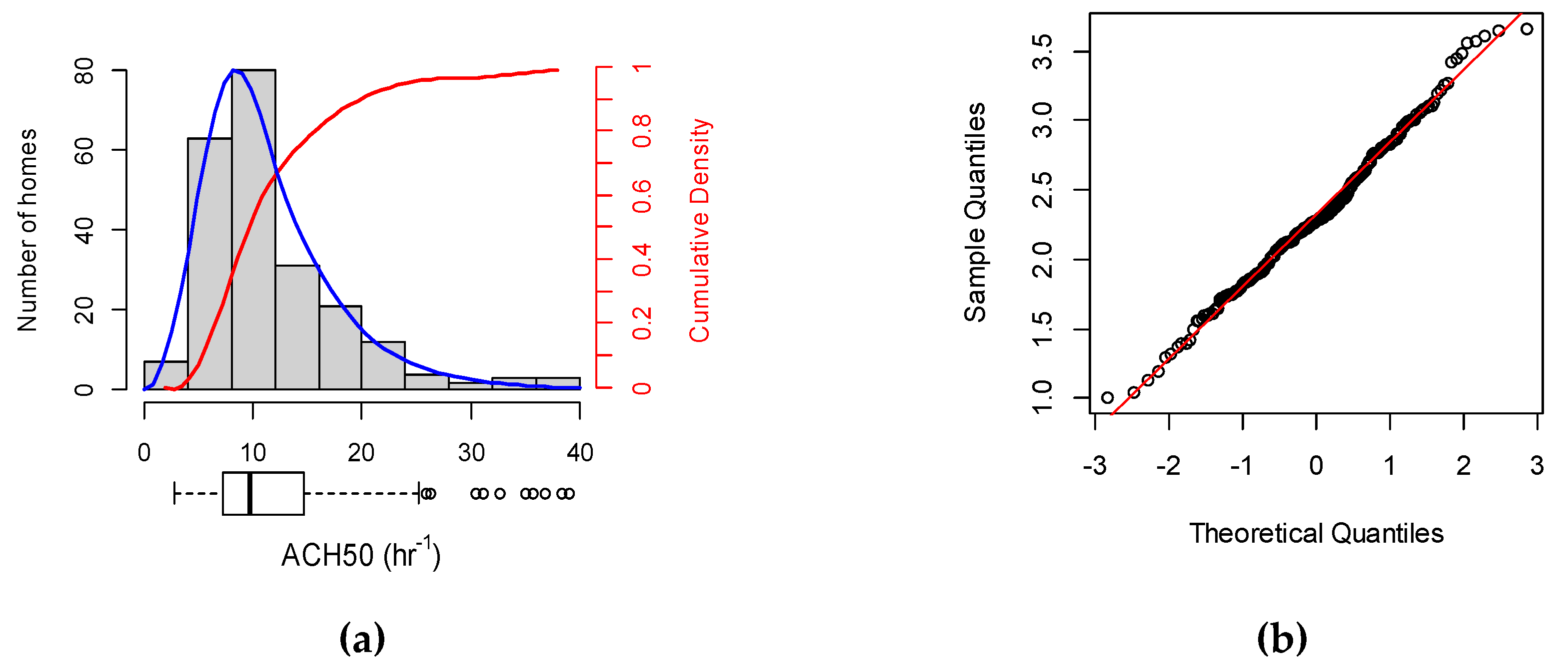
We used a combination of parametric and non-parametric approaches to estimate the relationships between building ventilation rates (measured as ACH50 and AAIR), building characteristics, and indoor air quality indicators. The variables ACH50 and AAIR were strongly correlated (
R2 = 0.92) and log-normally distributed (
Figure A1,
Appendix A); hence, they were log-transformed prior to further analyses like linear regressions or any statistical test of difference in distributions.
Data were analyzed using the R programming language (Version 3.4.4). Dummy variables were used when grouping the walk-through survey data into different categories. For continuous variables like ACH50, AAIR, and building volume, the sample distributions were firstly investigated using histogram plots. If the data showed distinct visual features like that of a normal or lognormal distribution, an Anderson–Darling (A–D) test was used in addition to quantile–quantile (Q–Q) plots to confirm the normal distribution of the data (or normality of log-transformed data). If the A–D test failed to reject the null hypothesis of the normality assumption (p > 0.05) in the sample distribution, a two-sample unpaired t-test with unequal variances was used to test for statistical difference in means between two groups and one-way analysis of variance (ANOVA) for more than two groups (tests performed on log-transformed data). As per the need, Tukey’s honest significant difference (Tukey HSD) post hoc test was conducted after ANOVA to investigate pair-wise significance in the difference of means between groups.
If a significant deviation (p < 0.05) from the normality assumption was reported by the A–D test, the non-parametric Kruskal–Wallis (K–W) test was used to assess differences in medians. Linear regression analyses were also performed to investigate the strength and statistical significance of association between the continuous variables of interest. Correlation between variables are reported as Pearson’s correlation coefficient (r). A level of significance of 5% (p = 0.05) was used in all the statistical tests and a p-value of >0.05 to 0.1 was defined as marginal significance.
Multivariable linear models were used to account for the variation in AAIR among the households due to potentially relevant parameters collected from the walk-through surveys, as well as the location and age of the homes. The variables were firstly tested using ANOVAs and simple regression models, and then the selected variables which individually showed significant correlations with AAIR were used in the multilinear models to predict ln(AAIR), since AAIR was found to be log-normally distributed.
Model 1 (Equation (2)) was developed to predict AAIR using only the E-scores, assuming the energy-efficient retrofits impacted the infiltration rate and to assess which retrofit was most effective.
where A
1 through A
5 represent each individual E-score,
is the intercept of the regression, β
1 through β
5 represent the coefficients of each predictor term that will be determined as a result of the regression analysis, and ε is the residual error term between the model prediction and the observed value.
Model 2 (Equation (3)) was constructed to evaluate the relative effects on AAIR introduced by building volume and age in addition to the E-scores, since these are known to impact infiltration rates in homes.
where the first six terms and ε are the same as in Model 1, Y represents the age of the building in years, and V represents the building volume in cubic feet. β
6, β
7, and β
8 are the regression coefficients of the age, volume, and age–volume interaction terms, respectively.
3. Results
The collected data on building air tightness, building characteristics, and healthy home indicators were analyzed to produce a set of qualitative and quantitative results relevant to the anticipated study outcomes.
3.1. Enrolled Study Homes
A total of 226 homes were enrolled in the CHEER study from low-income households located in the cities of Denver, Aurora, Boulder, Loveland, and Fort Collins. The study took place from 15 October 2015 to 15 April 2017. Due to missing data for some homes, 216 homes are presented in this paper.
The structural and envelope construction materials used in the study homes were primarily wood in the majority of homes (with concrete basement floors and basement walls) with less than one-quarter of the homes built with brick-masonry walls or a combination of wood and brick-masonry walls.
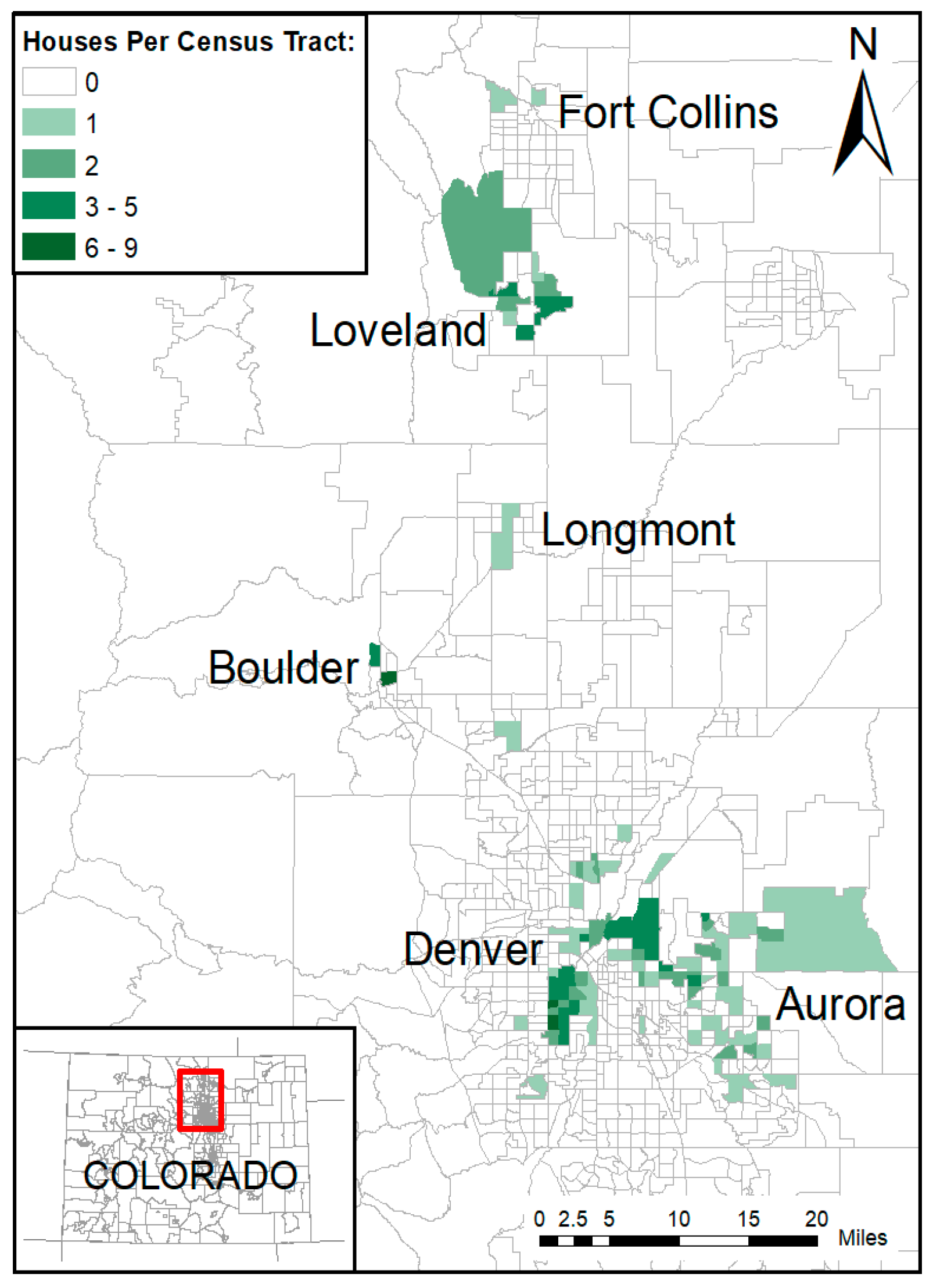
Figure 1 shows the spatial distribution of homes recruited for the CHEER study, which ranged from 1600 m to 1770 m above sea level in the International Energy Conservation Code climate zone 5 dry (B) region [
62]. The EER and non-EER homes were evenly distributed across all census tracts. Built green homes were located only in the Boulder and Loveland areas.
3.2. Household Characteristics
Table 1 summarizes the data on the various categories of building characteristics recorded during the walk-through surveys.
Of the 216 homes for which data were analyzed, 68% of the homes were constructed before 1976, the year when WAP began. Most homes (84%) were detached single-family buildings and were single-story (76%), and 46% of the homes were located within 200 m of a major road.
In terms of air-sealing measures observed in homes, the most common was door weather-stripping (72%) and the most infrequent was foam sealing of cracks and openings (17%). Very few homes (13%) had none of the air-sealing EERs visible from living spaces in the home. Many retrofits for energy efficiency were not observable by walk-through and included insulation blown into wall cavities and attics, caulking of attic floor level, and foam sealing of inaccessible crawl spaces.
Perceived indoor environmental quality survey results indicated that 38% of homes had air that was perceived by the surveyor as “not fresh” and 14% of homes had unacceptable odor levels. Also, almost 20% of homes had notable thermal variance between rooms. A past study also found that thermal and aural qualities in the indoor environment were deemed the most important contributors to the occupants’ acceptance of the overall indoor environmental quality, whereas indoor air quality was considered the least important [
63].
Visual cues observed during the walk-through surveys indicated that 9–57% of the homes had some form of an IEQ problem. More than half (57%) of the homes had stains somewhere on the walls, ceiling, or floor that were visible from the living space. About one-third (32%) of the homes also had mold growth that was directly visible from the living space. About one-fifth of the homes had dampness on the walls or floors, and 10% of the homes had condensation on the windows, both indicating potential mold problems. Almost half of the homes also had burnt candles indicating sources of indoor fine particulate matter and carbon monoxide. Most homes had either a recirculating stove hood or no stove hood and only 25% of the homes had stove hoods with outdoor exhaust (we did not ask how often these were used, however). The absence of exhaust-type stove hoods is particularly dangerous for occupant health in homes with gas stoves due to the risk of elevated carbon monoxide and nitrogen dioxide levels [
64].
3.3. Participant Demographics
The CHEER study homes were occupied by 303 inhabitants. Most of the occupants lived in the West Denver region (37% of the total number of occupants), were female (67%), non-Hispanic White (41%), and were 50 years or older (60%). A summary of the CHEER study occupant demographics is given in
Table A3 (
Appendix A).
3.4. Building Air Tightness
The average ACH50 for the CHEER study homes was 11.9 hr
−1 (standard deviation of 6.7 hr
−1) which is much lower than the average ACH50 value of 29.7 hr
−1 measured in 1998 across the US [
65], yet significantly higher compared to the 2012 International Energy Conservation Code’s requirement of 3 hr
−1 for new construction based on the climate of Colorado [
66].
The ASHRAE standard 119 [
67] uses normalized leakage as a metric for building leakage (and, consequently, air tightness). The average normalized leakage for our study homes was 0.72, which was 17% lower than the 1998 estimate for Colorado of 0.87 [
65], but 12.5% higher than the average value of 0.64 calculated from a database comprising of more than 70,000 homes in the US [
68].
The average AAIR of the CHEER study homes was 0.64 hr
−1 (standard deviation of 0.35 hr
−1). Linear regression results were found to be statistically significant between ln(AAIR) and building volume (
p < 0.001), and between ln(AAIR) and building age (
p < 0.001). This result is also consistent with past studies [
68,
69,
70].
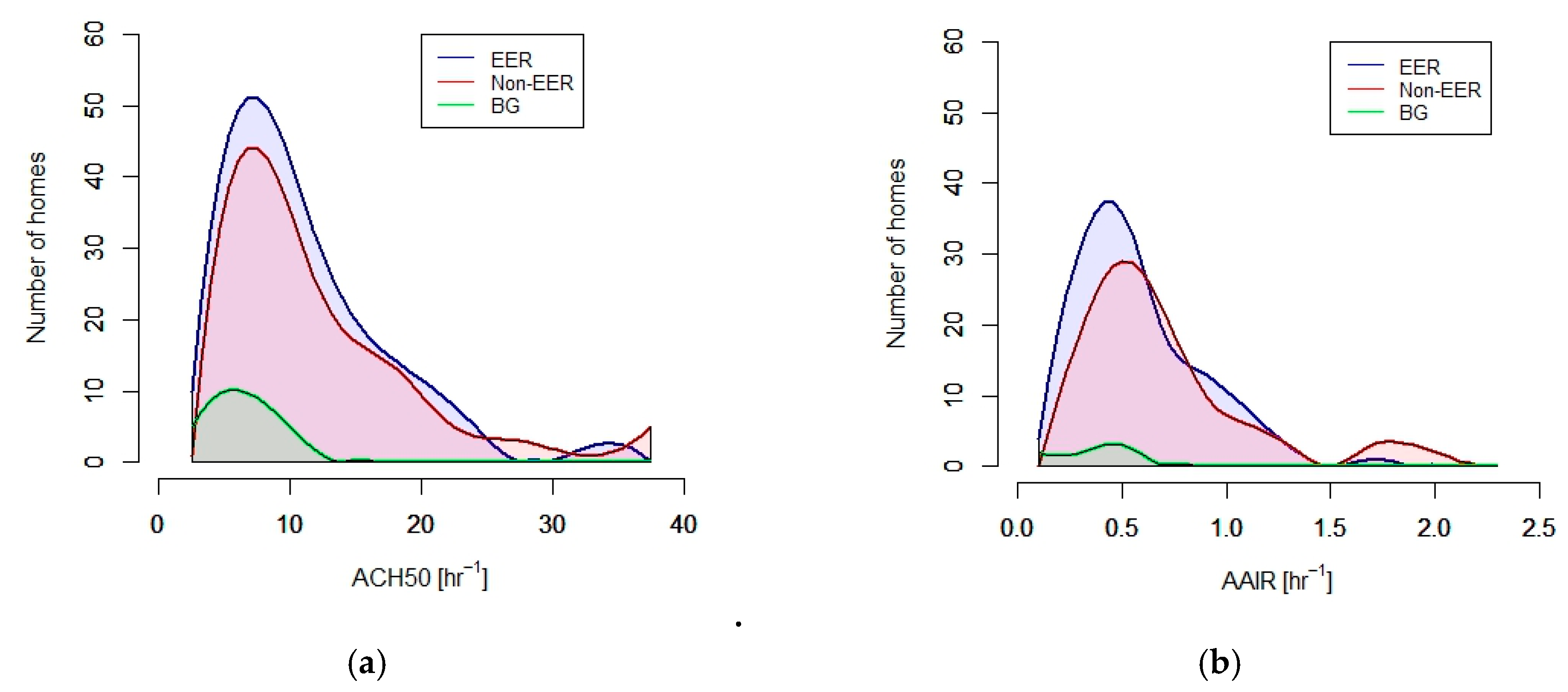
Although statistically different means in both ACH50 and AAIR were observed for the different building types, and the median AAIR of the EER homes was 17% lower than that of the non-EER homes (
Table 2), the overall distribution patterns of EER and non-EER homes were similar (
Figure 2).
AAIR was found to vary by location. Running a Tukey HSD post hoc test showed that the mean (± standard deviation) AAIR of West Denver homes (0.74 ± 0.36 hr−1) was higher (+54%) than Boulder/Fort Collins homes (0.48 ± 0.22 hr−1, p < 0.001), 23% higher than the Central/North Denver homes (0.60 ± 0.34 hr−1, p = 0.012), and 25% higher than Aurora homes (mean = 0.59 ± 0.34 hr−1, p = 0.065). Between other regions, mean AAIR values were not different.
3.5. E-Scores
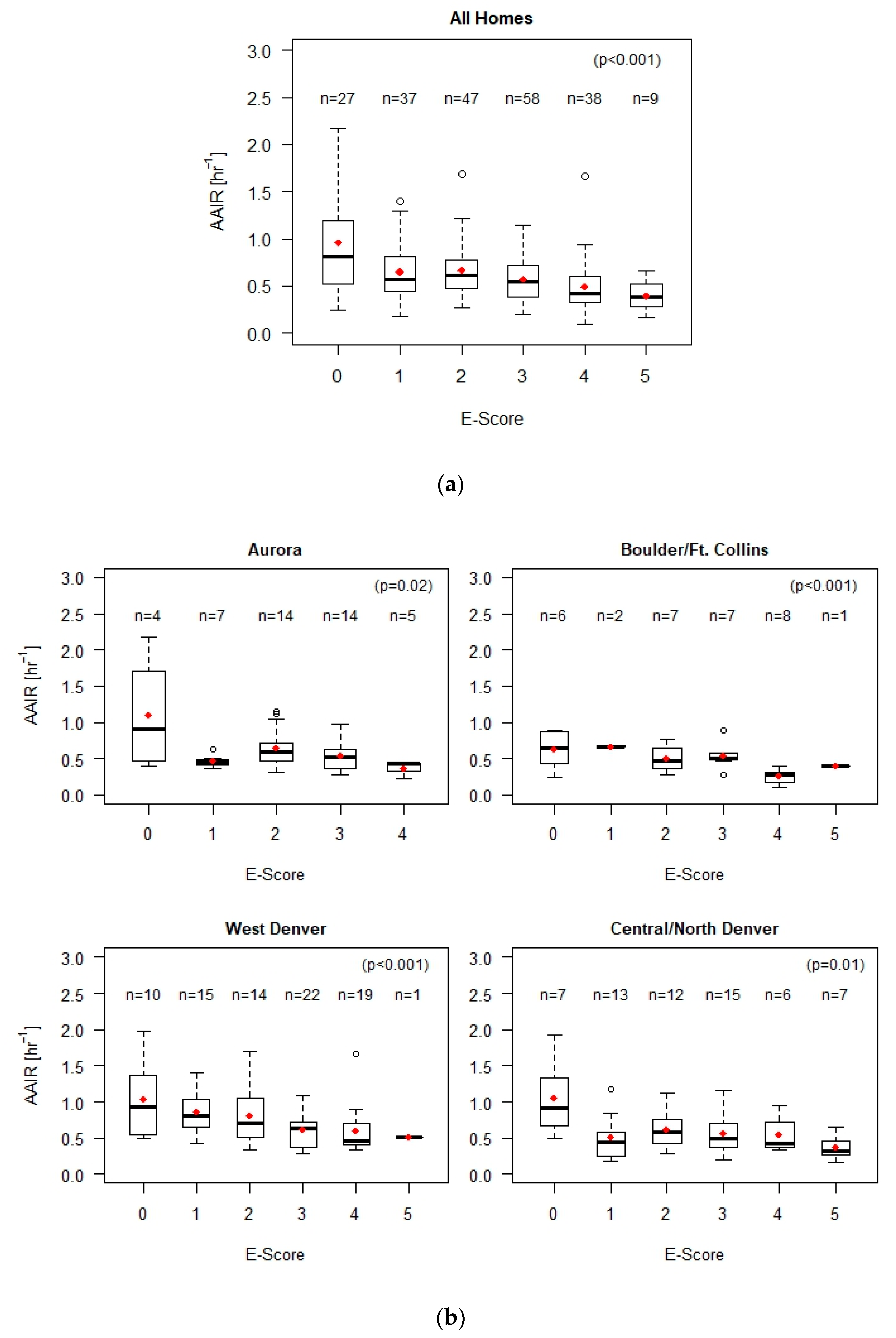
A negative relationship was found between E-score and AAIR (
Figure 3a). AAIR distributions had higher medians in most cases for E-scores of zero, compared to the median AAIRs in non-zero E-score categories. The changes in AAIR when the E-scores increased sequentially from one to five, however, were not monotonic in nature, and depended on the location of the homes (
Figure 3b).
Multilinear regression (Model 1, Equation (2)) showed a relationship between ln(AAIR) and E-score components (
p < 0.001) with normally distributed residuals. AAIRs were lower in homes where all the windows were weather-stripped and the air-handler ductwork was sealed. No differences in AAIR were seen in homes with other air-sealing EERs other than these two retrofits (
Table 3).
To investigate the combined effects of the air-sealing EERs and building age and volume, another multilinear regression was calculated (with Model 2, Equation (3)).
Table 4 shows that the contribution from air-sealing EERs toward AAIR was minimal compared to the contributions from building age and volume based on
p-value comparisons. However, air-handler ductwork sealing was found to still contribute in AAIR reduction among all the air-sealing EERs considered.
3.6. AAIR and Healthy Home Indicators
The differences in infiltration rates across different categories of healthy home indicators as noted in walk-through surveys are cross-tabulated in
Table 5.
4. Discussion
The median AAIRs of single-family homes ranged between 0.47 and 0.69 hr
−1 depending on the neighborhood across the Northern Front Range of Colorado US in which they were located. These results are comparable to the median air exchange rate estimated by perfluorocarbon tracer in Jew Jersey, Texas, and California, which was 0.71 hr
−1 overall. In Texas the cooling season median was lower (0.37 hr
−1) than the heating season (0.63 hr
−1); whereas, in California, the median was higher in summer (1.13 hr
−1) than in winter (0.61 hr
−1). These measurements account for window opening, whereas our estimates do not [
71]. The AAIRs in the CHEER study on single-family homes were 24% lower than in duplexes or townhomes. Single-family homes have all the exterior walls of the building available for direct infiltration of air from the surroundings, which is not the case in duplexes and townhomes. Intuitively, single-family homes should have a higher AAIR. However, it was found that single-family homes also had a median volume of 287 m
3, which was 35% higher than the median volume of duplexes/townhomes (213 m
3). Since we found an inverse relationship between AAIR and building volume, this explains the variation in median AAIR between the two categories. In addition, hidden passageways (through attics, crawlspaces, and wall cavities, for example) could have been present in duplexes and townhomes that could have affected the blower door test measurements. A sensitivity analysis of the main findings on the relationships between AAIR and various building characteristics was run for only single-family homes, but the final conclusions were not affected.
Building age also significantly impacted AAIR and ACH50 (data not shown). This result was reported by Sherman and Dickerhoff, who report that homes prior to 1980 were on average leakier and showed a clear increase in leakage with increasing age [
65]. According to Chan et al. (2005) [
72] who found similar results, some reasons why newer dwellings might tend to be tighter than older ones include improved materials (e.g., weather-stripped windows), better building techniques (e.g., air barriers), and lesser degrees of age-induced deterioration (e.g., settling of foundation).
Our result in
Table 3 agrees with past studies. In a study of 91 homes in Florida, 12–14% of house leaks were in the duct system, and duct repairs improved building tightness by decreasing the ACH50 from an average of 12 to 11, saving an annual average of
$200 in energy costs per home [
73]. A previous study of retrofit impacts in 465 US homes reported that the average retrofit reduced leakage by 25% [
65]. We did not have the opportunity to measure air tightness before any of our homes were retrofitted, as this was not part of the study design.
Our result in
Table 4 agrees with a previous study that found that floor area and year built were the most significant predictors of the building envelope leakage area [
72]. Buildings with greater volumes also indicate greater number of plumbing and higher probability of plumbing leakages that might lead to areas of moisture accumulation. This is especially true for older buildings that have need of a higher degree of repair, which, if not available, can again lead to moisture problems. The moisture accumulation in inaccessible areas like wall cavities can often lead to mold problems as well.
Referring to
Table 5, homes with a higher number of mold sightings during the walk-through surveys also had 12% higher median AAIRs. This was counter-intuitive to the conventional notion that tight homes can trap humidity indoors (generated from indoor sources like showering and cooking) for longer periods of time [
74]. Increased humidity can create favorable conditions of mold growth if the humid air condensates upon contact with cooler surfaces. One possible explanation for leakier homes with observations of mold growth could be that the leakier homes had a greater probability of outdoor mold spores infiltrating into the indoor environment. The mold spores could then find damp locations with stagnant air suitable for sustained mold growth and proliferation. Past studies found that most indoor fungi in homes come from outdoor air [
75]. Another major cause of mold in low income homes is leaky pipes or unseen leaks behind walls [
76], which would be another location for mold growth. Homes with observed mold growth were also found to be older with the median age of 66 years, compared to the median age of 58.5 years for homes with no mold growth observed.
Table 5 also shows that about half of CHEER homes had candles and the other half did not. We did not find an association between candle burning and AAIR, which meant that occupant behaviors like candle burning are mostly random, and occupants are generally not very cognizant about ventilation when they choose to burn candles indoors. Although occupant behavior like candle burning can directly affect indoor air quality, candle burning can be equally prevalent in both leakier and tighter homes. Hence, occupant behavior should also be largely accounted for in future studies to classify homes as “healthy” or “unhealthy”.
Based on dust level indoors indicated by the five-point MIDS, the homes with MIDS greater than 2.5 were also found to be on average 48% leakier than other study homes, which could have led to more outdoor air and particle infiltration. To investigate this possibility further, the homes with “high” versus “low” MIDS were compared with each other in terms of the mean distance of the home from the closest major road. It was found that the mean (± standard deviation) distance of high-MIDS homes from the closest major road was 189 ± 136 m, which was less than the low-MIDS homes, which was 294 ± 258 m (
p = 0.047). These results indicate that the leakier homes nearer to major roads have the potential to have higher outdoor dust levels infiltrating indoors. Much of this dust is traffic-related and could contain toxic components such as tire and brake wear, road paint [
77], and combustion-related particles such as black carbon [
78]. Many prior studies confirmed these results, whereby indoor particle concentrations are higher in homes that are closer to busy roadways [
79,
80,
81,
82].
Perceived indoor air quality responses showed marginal significance in terms of AAIR difference between the groups ordered according to acceptable odor level. It was observed that the homes in which indoor odor was reported by the surveyor as being “not acceptable” were 19% leakier than the homes with the odor perception being reported as “acceptable” or “somewhat acceptable”. This result is interesting and suggests that the odors could be related to outdoor air pollution. The median distance of the homes with an unacceptable odor level from the closest major road was 173 m, which was 24% lower than the median distance of other homes, which was 227 m (p = 0.53).

 ,
, 


