Multi-Objective Service Selection and Scheduling with Linguistic Preference in Cloud Manufacturing


Abstract
1. Introduction
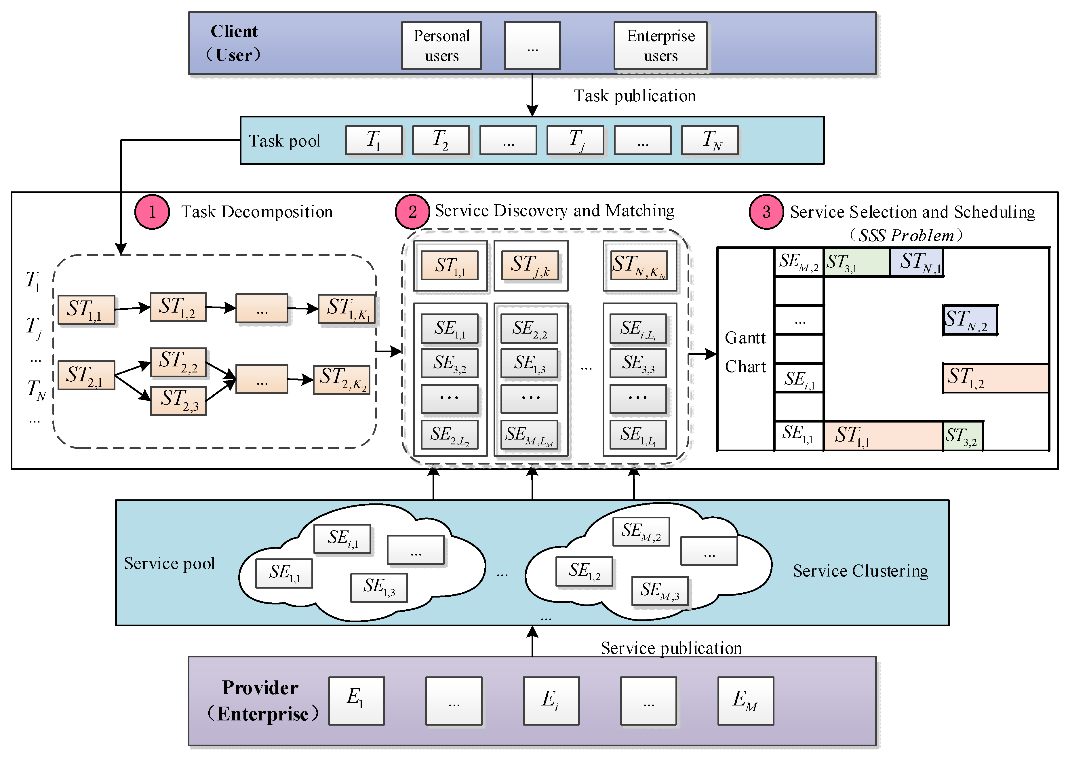
2. Problem Description
- Task decomposition: Manufacturing tasks in CMfg can be divided into simple tasks and complex tasks. Here, simple tasks can be assigned directly to available services, while complex tasks have to be decomposed into multiple subtasks, so that each subtask can be performed by a separate service [5,16]. There are four commonly accepted composition structures: sequential, parallel, selective, and loop [16,18,23].
- Service discovery and matching: for each subtask, the available services are found and put into the service set.
- Service selection and scheduling (SSS): for each subtask, one service is chosen from the corresponding service set, then these subtasks are scheduled onto the available time windows of selected services, and routes required transportations, such that the overall objectives are optimized.
3. The Multi-Objective Service Selection and Scheduling Model and Solution Methods
3.1. Assumptions
- All tasks are independent of each other.
- The service capabilities have been fully gathered in the given period.
- Each subtask has qualified service set and must be assigned to one service to complete.
- A started subtask cannot be interrupted.
- Before the SSS process, the service pool for each subtask has been built. Moreover, the time, cost, quality, and environmental cost of service for different services are already known.
- Only the sequence model is considered in this paper, which is just to simplify the calculation and does not affect the results of the study. Then, there is a precedence constraint relationship between various subtasks in a task.
- Consider a situation where there is only one DM.
3.2. Notations
- Service time of subtask , if subtask is assigned to service .
- Service cost of subtask , if subtask is assigned to service .
- Service quality of subtask , if subtask is assigned to service .
- Environmental cost of subtask , if subtask is assigned to service .
- Weight of products needed to be transported, if subtask is assigned to service .
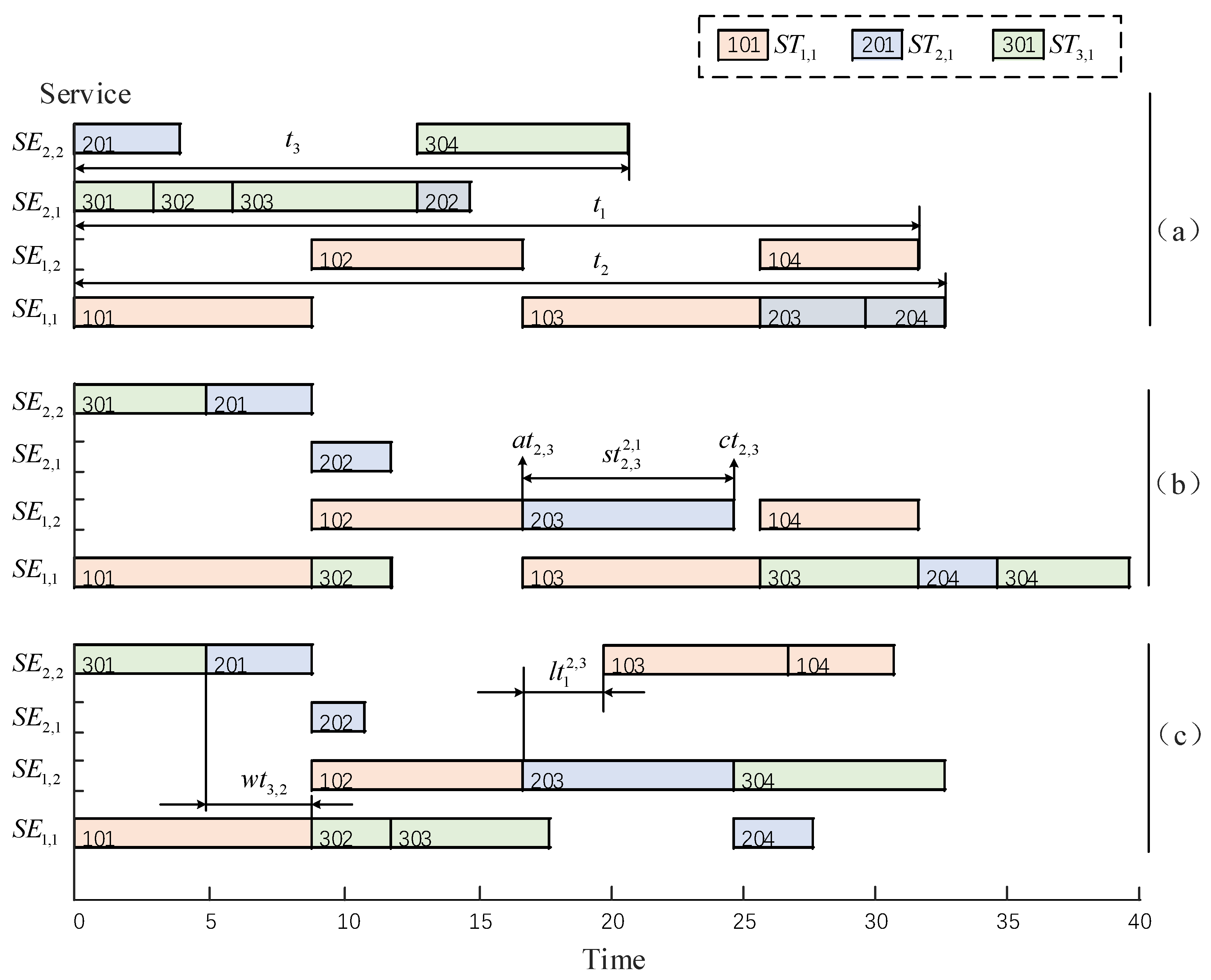
- Start time of subtask .
- Completion time of subtask .
- Waiting time of subtask .
- Logistics time from subtask to .
- Logistics cost from subtask to .
- Geographical distance between enterprises and .
- Logistics time for unit distance.
- Logistics cost for unit distance and unit weight.
3.3. Model Formulation
3.4. Optimization Algorithm
4. Computational Experiments and Results
4.1. A Small Scheduling Example
4.2. Computational Experiments
4.2.1. Data Generation
4.2.2. Define GA in Full Term
4.2.3. Test Results
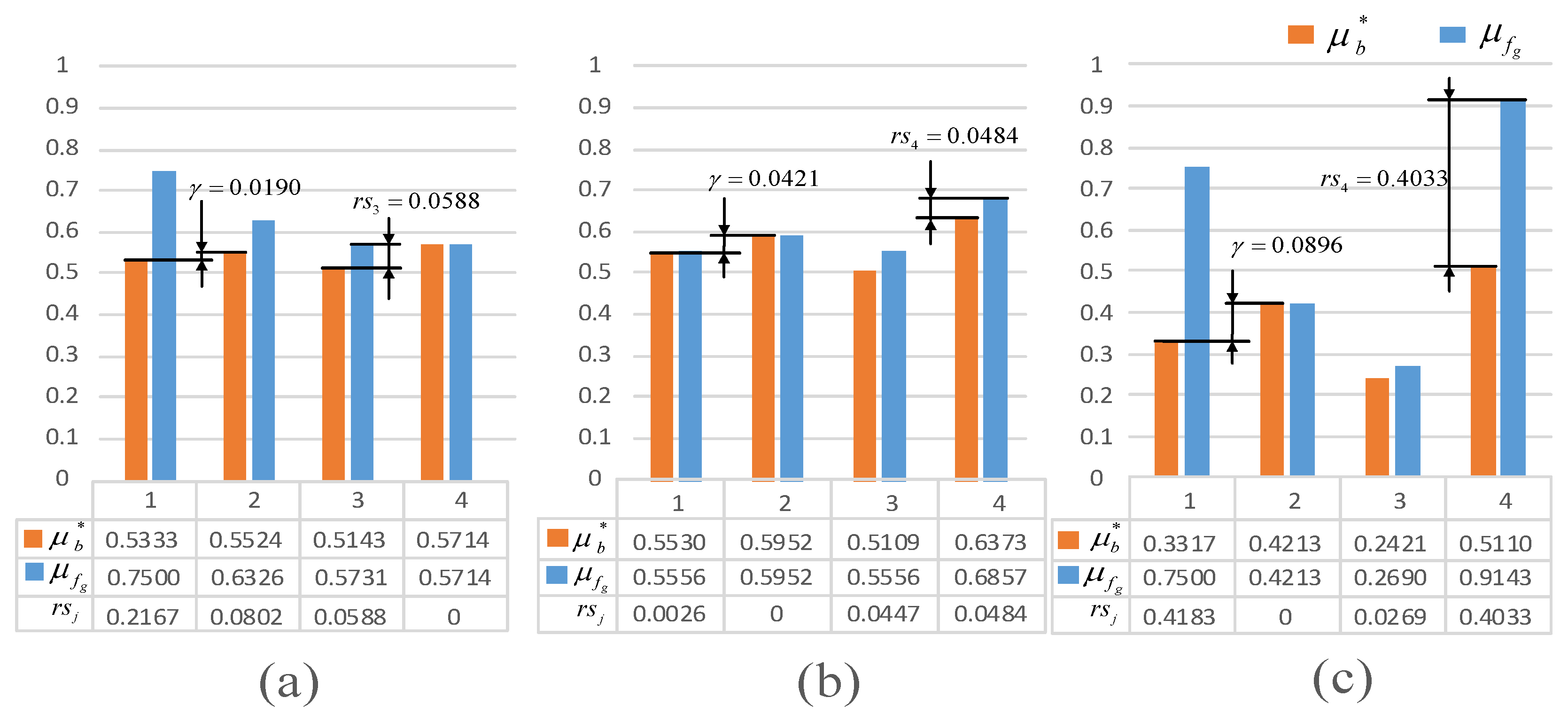
- : The desirable satisfying degree of the least important objectives, representing the overall optimization level of all objectives.
- γ: Parameter of importance, which means the difference of satisfying degree between objectives with different importance.
- rs: Redundant satisfying degree, which means the difference between an actual satisfying degree and a corresponding desirable satisfying degree.
4.3. Performance Stability of Different Scheduling Schemes
4.3.1. Different Scales of Services and Tasks/Subtasks
4.3.2. Different Numbers of Relative Importance Levels
5. Conclusions
Author Contributions
Funding
Acknowledgments
Conflicts of Interest
Appendix A

| T3 | SEi,h | [(1,1), (1,2), (2,1), (2,2)] | [(1,1), (1,2), (2,1), (2,2)] | [(1,1), (1,2), (2,1), (2,2)] | [(1,1), (1,2), (2,1), (2,2)] | |||||||||||||
| st | 9 | 9 | 8 | 9 | 5 | 8 | 10 | 7 | 9 | 10 | 5 | 7 | 7 | 6 | 8 | 4 | ||
| sc | 63 | 60 | 73 | 74 | 44 | 44 | 69 | 77 | 59 | 63 | 71 | 64 | 72 | 52 | 61 | 42 | ||
| q | 0.97 | 0.94 | 0.67 | 0.72 | 0.97 | 0.97 | 0.86 | 0.85 | 0.97 | 0.68 | 0.71 | 0.76 | 0.86 | 0.90 | 0.70 | 0.62 | ||
| ec | 6 | 14 | 14 | 14 | 13 | 7 | 8 | 6 | 6 | 15 | 8 | 6 | 6 | 7 | 15 | 5 | ||
| we | 22 | 18 | 22 | 19 | 22 | 18 | 22 | 21 | 24 | 22 | 19 | 23 | 21 | 19 | 25 | 17 | ||
| T2 | SEi,h | [(1,1), (1,2), (2,1), (2,2)] | [(1,1), (1,2), (2,1), (2,2)] | [(1,1), (1,2), (2,1), (2,2)] | [(1,1), (1,2), (2,1), (2,2)] | |||||||||||||
| st | 9 | 8 | 9 | 4 | 1 | 4 | 2 | 2 | 4 | 8 | 6 | 7 | 3 | 1 | 2 | 4 | ||
| sc | 44 | 78 | 75 | 55 | 73 | 66 | 78 | 41 | 63 | 71 | 42 | 80 | 54 | 69 | 74 | 68 | ||
| q | 0.91 | 0.61 | 0.63 | 0.90 | 0.62 | 0.52 | 0.58 | 0.50 | 0.97 | 0.50 | 0.82 | 0.95 | 0.72 | 0.67 | 0.92 | 0.62 | ||
| ec | 13 | 12 | 13 | 10 | 12 | 14 | 11 | 14 | 8 | 5 | 12 | 12 | 10 | 11 | 15 | 8 | ||
| we | 24 | 19 | 23 | 21 | 23 | 26 | 26 | 26 | 23 | 19 | 25 | 26 | 20 | 21 | 14 | 12 | ||
| T3 | SEi,h | [(1,1), (1,2), (2,1), (2,2)] | [(1,1), (1,2), (2,1), (2,2)] | [(1,1), (1,2), (2,1), (2,2)] | [(1,1), (1,2), (2,1), (2,2)] | |||||||||||||
| st | 4 | 2 | 3 | 5 | 3 | 7 | 3 | 3 | 6 | 4 | 7 | 6 | 5 | 8 | 8 | 8 | ||
| sc | 58 | 76 | 45 | 55 | 50 | 75 | 67 | 55 | 58 | 60 | 75 | 76 | 54 | 69 | 72 | 49 | ||
| q | 0.56 | 0.65 | 0.68 | 0.95 | 0.64 | 0.53 | 0.63 | 0.68 | 1.00 | 0.89 | 0.91 | 0.74 | 0.89 | 0.71 | 0.83 | 0.82 | ||
| ec | 10 | 14 | 5 | 5 | 6 | 12 | 7 | 12 | 7 | 8 | 12 | 11 | 14 | 8 | 13 | 9 | ||
| we | 15 | 19 | 15 | 15 | 17 | 17 | 14 | 12 | 28 | 23 | 22 | 22 | 18 | 20 | 20 | 17 | ||
| Enterprise | E1 | E2 |
|---|---|---|
| 0 | 222 | |
| 222 | 0 |
References
- Li, B.; Zhang, L.; Wang, S.; Tao, F.; Cao, J.; Jiang, X.; Song, X.; Cai, X. Cloud manufacturing: A new service-oriented networked manufacturing model. Comput. Integr. Manuf. Syst. 2010, 16, 1–7. (In Chinese) [Google Scholar]
- He, W.; Xu, L. A state-of-the-art survey of cloud manufacturing. Int. J. Comput. Integr. Manuf. 2015, 28, 239–250. [Google Scholar] [CrossRef]
- Chen, J.; Huang, G.Q.; Wang, J.; Yang, C. A cooperative approach to service booking and scheduling in cloud manufacturing. Eur. J. Oper. Res. 2019, 273, 861–873. [Google Scholar] [CrossRef]
- Tao, F.; Zhang, L.; Liu, Y.; Cheng, Y.; Wang, L.; Xu, X. Manufacturing Service Management in Cloud Manufacturing: Overview and Future Research Directions. J. Manuf. Sci. Eng. 2015, 137, 040912. [Google Scholar] [CrossRef]
- Tao, F.; LaiLi, Y.; Xu, L.; Zhang, L. FC-PACO-RM: A parallel method for service composition optimal-selection in cloud manufacturing system. IEEE Trans. Ind. Inform. 2013, 9, 2023–2033. [Google Scholar] [CrossRef]
- Xu, X. From cloud computing to cloud manufacturing. Robot. Comput.-Integr. Manuf. 2012, 28, 75–86. [Google Scholar] [CrossRef]
- Zhang, Y.; Zhang, G.; Liu, Y.; Hu, D. Research on services encapsulation and virtualization access model of machine for cloud manufacturing. J. Intell. Manuf. 2017, 28, 1109–1123. [Google Scholar] [CrossRef]
- Cheng, Y.; Tao, F.; Zhao, D.; Zhang, L. Modeling of manufacturing service supply-demand matching hypernetwork in service-oriented manufacturing systems. Robot. Comput.-Integr. Manuf. 2017, 45, 59–72. [Google Scholar] [CrossRef]
- Shen, X.; Yao, X. Mathematical modeling and multi-objective evolutionary algorithms applied to dynamic flexible job shop scheduling problems. Inform. Sci. 2015, 298, 198–224. [Google Scholar] [CrossRef]
- Wang, S.; Guo, L.; Kang, L.; Li, C.; Li, X.; Stephane, Y.M. Research on selection strategy of machining equipment in cloud manufacturing. Int. J. Adv. Manuf. Technol. 2014, 71, 1549–1563. [Google Scholar] [CrossRef]
- Liu, W.; Liu, B.; Sun, D.; Li, Y.; Ma, G. Study on multi-task oriented services composition and optimisation with the “Multi-Composition for Each Task’ pattern in cloud manufacturing systems. Int. J. Comput. Integr. Manuf. 2013, 26, 786–805. [Google Scholar] [CrossRef]
- Tao, F.; Cheng, J.; Cheng, Y.; Gu, S.; Zheng, T.; Yang, H. SDMSim: A manufacturing service supply-demand matching simulator under cloud environment. Robot. Comput.-Integr. Manuf. 2017, 45, 34–46. [Google Scholar] [CrossRef]
- Chen, T. Strengthening the competitiveness and sustainability of a semiconductor manufacturer with cloud manufacturing. Sustainability 2014, 6, 251–266. [Google Scholar] [CrossRef]
- Wu, D.; Greer, M.J.; Rosen, D.W.; Schaefer, D. Cloud manufacturing: Strategic vision and state-of-the-art. J. Manuf. Syst. 2013, 32, 564–579. [Google Scholar] [CrossRef]
- Liu, Y.; Xu, X.; Zhang, L.; Wang, L.; Zhong, R.Y. Workload-based multi-task scheduling in cloud manufacturing. Robot. Comput.-Integr. Manuf. 2017, 45, 3–20. [Google Scholar] [CrossRef]
- Akbaripour, H.; Houshmand, M.; van Woensel, T.; Mutlu, N. Cloud manufacturing service selection optimization and scheduling with transportation considerations: Mixed-integer programming models. Int. J. Adv. Manuf. Technol. 2018, 95, 43–70. [Google Scholar] [CrossRef]
- Cheng, Y.; Tao, F.; Liu, Y.; Zhao, D.; Zhang, L.; Xu, L. Energy-aware resource service scheduling based on utility evaluation in cloud manufacturing system. Proc. Inst. Mech. Eng. B J. Eng. 2013, 227, 1901–1915. [Google Scholar] [CrossRef]
- Huang, B.; Li, C.; Tao, F. A chaos control optimal algorithm for QoS-based service composition selection in cloud manufacturing system. Enterp. Inf. Syst. UK 2014, 8, 445–463. [Google Scholar] [CrossRef]
- Xiang, F.; Hu, Y.; Yu, Y.; Wu, H. QoS and energy consumption aware service composition and optimal-selection based on Pareto group leader algorithm in cloud manufacturing system. Cent. Eur. J. Oper. Res. 2014, 22, 663–685. [Google Scholar] [CrossRef]
- Li, C.; Wang, S.; Kang, L.; Guo, L.; Cao, Y. Trust evaluation model of cloud manufacturing service platform. Int. J. Adv. Manuf. Technol. 2014, 75, 489–501. [Google Scholar] [CrossRef]
- Lartigau, J.; Xu, X.; Nie, L.; Zhan, D. Cloud manufacturing service composition based on QoS with geo-perspective transportation using an improved Artificial Bee Colony optimisation algorithm. Int. J. Prod. Res. 2015, 53, 4380–4404. [Google Scholar] [CrossRef]
- Ahn, G.; Park, Y.; Hur, S. The dynamic enterprise network composition algorithm for efficient operation in cloud manufacturing. Sustainability 2016, 8, 1239. [Google Scholar] [CrossRef]
- Tao, F.; Zhao, D.; Hu, Y.; Zhou, Z. Correlation-aware resource service composition and optimal-selection in manufacturing grid. Eur. J. Oper. Res. 2010, 201, 129–143. [Google Scholar] [CrossRef]
- Wu, Z.; Liu, T.; Gao, Z.; Cao, Y.; Yang, J. Tolerance design with multiple resource suppliers on cloud-manufacturing platform. Int. J. Adv. Manuf. Technol. 2016, 84, 335–346. [Google Scholar] [CrossRef]
- Cao, Y.; Wang, S.; Kang, L.; Gao, Y. A TQCS-based service selection and scheduling strategy in cloud manufacturing. Int. J. Adv. Manuf. Technol. 2016, 82, 235–251. [Google Scholar] [CrossRef]
- Hwang, C.L.; Masud, A.S.M. Multiple Objective Decision Making—Methods and Applications; Springer: New York, NY, USA, 1979. [Google Scholar]
- Narasimhan, R. GOAL PROGRAMMING IN A FUZZY ENVIRONMENT. Decis. Sci. 2010, 11, 325–336. [Google Scholar] [CrossRef]
- Chen, L.H.; Tsai, F.C. Fuzzy goal programming with different importance and priorities. Eur. J. Oper. Res. 2001, 133, 548–556. [Google Scholar] [CrossRef]
- Abdelmaguid, T.F.; Nassef, A.O.; Kamal, B.A.; Hassan, M.F. A hybrid GA/heuristic approach to the simultaneous scheduling of machines and automated guided vehicles. Int. J. Prod. Res. 2004, 42, 267–281. [Google Scholar] [CrossRef]
- Liu, L.; Hu, R.; Hu, X.; Zhao, G.; Wang, S. A hybrid PSO-GA algorithm for job shop scheduling in machine tool production. Int. J. Prod. Res. 2015, 53, 5755–5781. [Google Scholar] [CrossRef]
- Falzon, G.; Li, M. Enhancing genetic algorithms for dependent job scheduling in grid computing environments. J. Supercomput. 2012, 62, 290–314. [Google Scholar] [CrossRef]


| Desirable Satisfying Degree | Satisfying Degree | |||
|---|---|---|---|---|
| 0.95 | 0.011 | [0.547 0.558 0.536 0.569] | [0.731 0.558] 0.598 0.718] | 0.396 |
| 0.9 | 0.058 | [0.577 0.635 0.519 0.692] | [0.577 0.681 0.602 0.718] | 0.156 |
| 0.85 | 0.059 | [0.575 0.634 0.517 0.692] | [0.577 0.694 0.555 0.692] | 0.101 |
| 0.8 | 0.086 | [0.547 0.633 0.462 0.718] | [0.577 0.715 0.469 0.718] | 0.120 |
| 0.75 | 0.086 | [0.547 0.633 0.462 0.718] | [0.615 0.704 0.608 0.718] | 0.286 |
| 0.7 | 0.089 | [0.514 0.603 0.425 0.692] | [0.577 0.694 0.555 0.692] | 0.283 |
| [1,10] | [40,80] | [0.5,1] | [5,15] | [10,30] | [1,500] |
| Dataset | ∆δ | Max-min | Two-phase | Weighted Sum | |||||||||
|---|---|---|---|---|---|---|---|---|---|---|---|---|---|
| γ | rs | CPU(s) | γ | rs | CPU(s) | γ | rs | CPU(s) | |||||
| 6s5t8st | 0.9 | 0.476 | 0.030 | 0.115 | 0.881 | 0.491 | 0.032 | 0.129 | 1.252 | 0.396 | 0.038 | 0.664 | 0.901 |
| 0.7 | 0.386 | 0.086 | 0.147 | 0.931 | 0.377 | 0.093 | 0.159 | 11.938 | 0.283 | 0.101 | 0.703 | 0.941 | |
| 6s10t10st | 0.9 | 0.436 | 0.028 | 0.173 | 2.034 | 0.426 | 0.032 | 0.097 | 2.384 | 0.293 | 0.031 | 0.889 | 2.041 |
| 0.7 | 0.341 | 0.079 | 0.254 | 2.108 | 0.336 | 0.101 | 0.135 | 15.25 | 0.265 | 0.093 | 0.717 | 2.066 | |
| 6s15t12st | 0.9 | 0.439 | 0.034 | 0.169 | 3.389 | 0.446 | 0.044 | 0.144 | 3.668 | 0.197 | 0.211 | 0.577 | 3.558 |
| 0.7 | 0.345 | 0.082 | 0.386 | 3.340 | 0.336 | 0.116 | 0.212 | 18.083 | 0.119 | 0.267 | 0.638 | 3.538 | |
| 12s5t10st | 0.9 | 0.512 | 0.020 | 0.203 | 1.060 | 0.524 | 0.025 | 0.108 | 1.591 | 0.281 | 0.114 | 0.496 | 1.100 |
| 0.7 | 0.412 | 0.062 | 0.301 | 1.087 | 0.408 | 0.071 | 0.226 | 19.172 | 0.243 | 0.155 | 0.416 | 1.063 | |
| 12s10t12st | 0.9 | 0.452 | 0.022 | 0.189 | 2.289 | 0.439 | 0.022 | 0.152 | 2.524 | 0.283 | 0.030 | 0.985 | 2.285 |
| 0.7 | 0.329 | 0.054 | 0.259 | 2.533 | 0.321 | 0.068 | 0.152 | 9.450 | 0.136 | 0.050 | 1.241 | 2.492 | |
| 12s15t12st | 0.9 | 0.453 | 0.029 | 0.142 | 3.59 | 0.440 | 0.037 | 0.128 | 4.323 | 0.192 | 0.110 | 0.688 | 3.621 |
| 0.7 | 0.355 | 0.064 | 0.334 | 4.018 | 0.345 | 0.100 | 0.133 | 32.194 | 0.153 | 0.168 | 0.503 | 3.580 | |
| 18s5t8st | 0.9 | 0.430 | 0.052 | 0.155 | 0.950 | 0.443 | 0.075 | 0.165 | 1.381 | 0.325 | 0.125 | 0.694 | 1.023 |
| 0.7 | 0.356 | 0.155 | 0.235 | 1.049 | 0.374 | 0.189 | 0.167 | 13.606 | 0.250 | 0.177 | 1.009 | 0.940 | |
| 18s10t8st | 0.9 | 0.408 | 0.019 | 0.142 | 1.655 | 0.408 | 0.019 | 0.111 | 1.882 | 0.213 | 0.012 | 1.267 | 1.637 |
| 0.7 | 0.325 | 0.051 | 0.166 | 1.666 | 0.340 | 0.061 | 0.099 | 9.125 | 0.203 | 0.044 | 1.036 | 1.702 | |
| 18s15t10st | 0.9 | 0.480 | 0.027 | 0.159 | 3.190 | 0.487 | 0.036 | 0.119 | 3.492 | 0.297 | 0.070 | 0.950 | 3.260 |
| 0.7 | 0.350 | 0.065 | 0.270 | 3.532 | 0.368 | 0.080 | 0.144 | 13.430 | 0.217 | 0.085 | 0.842 | 3.242 | |
| Dataset | ∆δ | Max-min | Two-phase | Weighted Sum | |||||||||
|---|---|---|---|---|---|---|---|---|---|---|---|---|---|
| γ | rs | CPU(s) | γ | rs | CPU(s) | γ | rs | CPU(s) | |||||
| 60s15t15st | 0.9 | 0.472 | 0.057 | 0.210 | 4.729 | 0.470 | 0.090 | 0.143 | 5.317 | 0.401 | 0.147 | 0.554 | 4.611 |
| 0.7 | 0.362 | 0.161 | 0.400 | 4.229 | 0.364 | 0.206 | 0.231 | 44.98 | 0.288 | 0.197 | 0.886 | 5.093 | |
| 600s15t15st | 0.9 | 0.405 | 0.015 | 0.247 | 4.746 | 0.412 | 0.019 | 0.180 | 4.939 | 0.180 | 0.018 | 1.506 | 4.257 |
| 0.7 | 0.346 | 0.052 | 0.314 | 5.014 | 0.341 | 0.057 | 0.242 | 16.57 | 0.084 | 0.031 | 1.690 | 4.416 | |
| 600s15t30st | 0.9 | 0.460 | 0.024 | 0.169 | 10.61 | 0.437 | 0.023 | 0.183 | 10.35 | 0.285 | 0.032 | 0.925 | 9.817 |
| 0.7 | 0.331 | 0.050 | 0.343 | 9.724 | 0.345 | 0.070 | 0.246 | 42.96 | 0.202 | 0.084 | 0.841 | 9.318 | |
| 600s30t15st | 0.9 | 0.463 | 0.023 | 0.245 | 10.20 | 0.444 | 0.026 | 0.200 | 12.47 | 0.233 | 0.153 | 0.566 | 10.90 |
| 0.7 | 0.325 | 0.051 | 0.166 | 1.666 | 0.340 | 0.061 | 0.099 | 9.125 | 0.203 | 0.044 | 1.036 | 1.702 | |
| 600s50t50st | 0.9 | 0.423 | 0.019 | 0.131 | 112.7 | 0.401 | 0.018 | 0.131 | 114.1 | 0.281 | 0.024 | 0.844 | 112.2 |
| 0.7 | 0.302 | 0.045 | 0.222 | 113.4 | 0.313 | 0.063 | 0.124 | 246.5 | 0.157 | 0.060 | 0.830 | 118.7 | |
| Level | ∆δ | Max-min | Two-phase | Weighted Sum | |||||||||
|---|---|---|---|---|---|---|---|---|---|---|---|---|---|
| γ | rs | CPU(s) | γ | rs | CPU(s) | γ | rs | CPU(s) | |||||
| 3 | 0.9 | 0.474 | 0.035 | 0.158 | 2.416 | 0.465 | 0.046 | 0.163 | 3.222 | 0.250 | 0.220 | 0.371 | 2.369 |
| 0.7 | 0.365 | 0.089 | 0.351 | 2.566 | 0.362 | 0.121 | 0.164 | 14.992 | 0.185 | 0.278 | 0.477 | 2.352 | |
| 4 | 0.9 | 0.450 | 0.018 | 0.167 | 2.402 | 0.487 | 0.027 | 0.124 | 2.724 | 0.249 | 0.023 | 1.129 | 2.368 |
| 0.7 | 0.361 | 0.054 | 0.276 | 2.676 | 0.350 | 0.070 | 0.142 | 15.191 | 0.145 | 0.057 | 1.205 | 2.542 | |
| 5 | 0.9 | 0.446 | 0.014 | 0.117 | 2.247 | 0.452 | 0.018 | 0.121 | 2.581 | 0.193 | 0.010 | 1.401 | 2.240 |
| 0.7 | 0.353 | 0.043 | 0.187 | 2.333 | 0.356 | 0.047 | 0.118 | 15.812 | 0.175 | 0.034 | 1.185 | 2.447 | |
| 6 | 0.9 | 0.464 | 0.016 | 0.164 | 2.472 | 0.449 | 0.027 | 0.567 | 3.214 | 0.142 | 0.052 | 1.171 | 2.426 |
| 0.7 | 0.358 | 0.042 | 0.350 | 2.551 | 0.349 | 0.062 | 0.545 | 20.836 | 0.125 | 0.107 | 0.784 | 2.301 | |
| 7 | 0.9 | 0.461 | 0.012 | 0.189 | 2.381 | 0.470 | 0.018 | 0.572 | 2.892 | 0.135 | 0.035 | 1.097 | 2.375 |
| 0.7 | 0.356 | 0.032 | 0.350 | 2.592 | 0.356 | 0.050 | 0.510 | 22.373 | 0.092 | 0.048 | 1.114 | 2.375 | |
© 2019 by the authors. Licensee MDPI, Basel, Switzerland. This article is an open access article distributed under the terms and conditions of the Creative Commons Attribution (CC BY) license (http://creativecommons.org/licenses/by/4.0/).
Share and Cite
He, W.; Jia, G.; Zong, H.; Kong, J. Multi-Objective Service Selection and Scheduling with Linguistic Preference in Cloud Manufacturing. Sustainability 2019, 11, 2619. https://doi.org/10.3390/su11092619
He W, Jia G, Zong H, Kong J. Multi-Objective Service Selection and Scheduling with Linguistic Preference in Cloud Manufacturing. Sustainability. 2019; 11(9):2619. https://doi.org/10.3390/su11092619
Chicago/Turabian StyleHe, Wei, Guozhu Jia, Hengshan Zong, and Jili Kong. 2019. "Multi-Objective Service Selection and Scheduling with Linguistic Preference in Cloud Manufacturing" Sustainability 11, no. 9: 2619. https://doi.org/10.3390/su11092619
APA StyleHe, W., Jia, G., Zong, H., & Kong, J. (2019). Multi-Objective Service Selection and Scheduling with Linguistic Preference in Cloud Manufacturing. Sustainability, 11(9), 2619. https://doi.org/10.3390/su11092619