Is South Korea’s Emission Trading Scheme Effective? An Analysis Based on the Marginal Abatement Cost of Coal-Fueled Power Plants

Abstract

This paper examines not only the effectiveness of the South Korean emissions-trading scheme (ETS), but also the determinants of its performance. We apply a directional distance function and stochastic frontier analysis method to estimate environmental efficiency and the marginal CO₂ abatement costs for 50 coal-fueled power plants from 2008 to 2016. The result indicates that the efficiency differs between the Lee Myung-bak and Park Geun-hye administration periods, with performance in the former period being relatively more effective than in the latter. Meanwhile, there were price gaps of 57.98% and 72.76% in 2015 and 2016, respectively, between the realized carbon market price and our result, indicating significant suppressed pressure on the market. We conclude that the Korean government should strengthen its regulations to more effectively implement a green economy. Policymakers could impose a carbon tax; substantially decrease the carbon emissions-free quota; and provide more incentives, especially to the energy-intensive, resource-saving coal-fueled power plants. This would ultimately keep market prices within a reasonable range and achieve a balance between the supply and demand for carbon emission allowances in the market.

1. Introduction

The global environmental problem, and especially the greenhouse effect caused by carbon dioxide emissions, has worsened in the 21st century. To stabilize the atmospheric concentration of CO₂ and avoid serious climate change, global emissions must be reduced by roughly 80% from business as usual (BAU) levels over the next several decades. The Paris Agreement adopted in 2015 established specific actions and targets for reducing greenhouse gas emissions to mitigate and adapt to the effects of climate change [1]. The Paris Agreement also proposed controls to keep the average global temperature to within 2 °C of pre-Industrial Revolution levels in an attempt to limit this increase to 1.5 °C; this will greatly reduce the risk and influence of climate change. Further, the 2018 United Nations Climate Change Conference (COP 24) in Katowice, Poland, resulted in a “Paris Rulebook” for the forceful implementation of the Paris Agreement [2] across all countries in 2018.

Several emissions-trading schemes (ETSs) have been established to reduce CO₂ emissions, such as the EU ETS, California-Quebec ETS, and New Zealand ETS, among others. The ETS provides a way to reduce pollutant emissions using market measures, which is more scientific and effective than compulsory administrative measures.

Korea is the 11th largest economy worldwide, and consumed approximately 2.2% of the world’s total primary energy in 2017, making it the eighth-largest global energy consumer. Moreover, Korea accounted for 2.3% of global coal consumption in 2017, or sixth worldwide [3]. To shoulder more of its various responsibilities—from curtailing global carbon emissions to relieving burdens on the domestic environment—the Korean government established its “low carbon-green growth” national carbon-reduction policy in 2009, then passed a law mandating decreased national CO₂ emissions by 30% below business as usual (BAU) levels by 2020. Under this framework, the Korean government in 2012 also established a “Management of Targets for GHGs (greenhouse gases) and Energy” system to set goals for reducing GHGs and energy use among industries and power generators, and to manage and support their implementation. Meanwhile, as a concrete way to reduce emissions, the Korean National Assembly approved a carbon emissions-trading scheme in 2012; after a long policy-making period, this scheme formally began in 2015. The main compliance tools under the carbon ETS involve directly decreasing CO₂ emissions and purchasing emission allowances, and thus, power plants must be well-versed in these two measures’ costs and benefits. Prudent decisions about allowance trading based on accurate information can prevent rash transactions that could damage a company’s financial condition. Thus, the most essential work for coal-fueled power plants involves not only making abatement decisions by examining the potential gains from such abatement, but also procuring allowances according to their marginal abatement cost (MAC). The MAC presents an estimated value of the opportunity cost for undesirable output, while providing meaningful guidelines to formulate regulatory policies for public decision-makers [4].

In recent years, carbon dioxide emissions caused by global warming as well as energy shortages and their associated environmental problems have become the focus of the world’s attention. Governments worldwide have fought to cut the amount of greenhouse gases—such as carbon dioxide, methane, nitric oxide, and fluorocarbons—that are being pumped into the atmosphere. Coal resources produce the most carbon dioxide per unit of energy among all fossil fuels; thus, burning coal poses a further threat to the global climate, which is already warming at an alarming rate. The carbon dioxide exhaust from coal-fired power stations contribute to approximately 10% of all carbon dioxide emissions [5].

Korea’s coal-fueled power plants have the potential to play a key role in reducing carbon emissions, as they account for 43% of the nation’s electricity generation and approximately 25% of its total carbon emissions. The energy and electricity-generation sectors collectively account for 43.6% of the ETS market’s total quota, and thus, the Korean ETS’ effectiveness should be based on that of the coal-fueled power industry. Therefore, this research focuses on the coal-fueled power industry’s environment efficiency, and its MAC to reduce carbon emissions.

Over the past two decades, substantial empirical studies worldwide have examined pollutants’ MAC and the coal-fueled power sector’s efficiency [6,7,8,9,10,11,12,13]. However, few empirical studies have attempted to analyze this field in Korea [14,15,16,17,18]. Studies of coal pollutants’ MAC have been especially scarce after the Korean ETS’ establishment, at least until now. We provide two contributions to fill these gaps from previous studies. First, the random error and statistic noise have long been ignored in previous studies; therefore, we introduce a stochastic frontier analysis (SFA) approach in this field to obtain more accurate results. Second, we collect a recent dataset that includes information before and after the Korean ETS’ establishment to conduct longitudinal time-series study. This will reveal the ETS policies’ effectiveness on the participating coal-power industry.

The remainder of this study is organized as follows: Section 2 summarizes trends among pollutants’ MAC, efficiency performance estimation methods, and related studies. Section 3 then illustrates the theoretical methodology. Section 4 notes the variables and data, then discusses the empirical results. Section 5 concludes and provides policy implications.

2. Literature Review

Studies on pollutants’ MAC and their potential abatement have continuously improved and become more numerous during the past few decades. Schmidt [19] and Aigner and Chu [20] first used the production function to estimate pollutants’ MAC, while Pollak et al. [21] and Gollop et al. [22] subsequently estimated pollutants’ MAC using a cost function.

In the last 20 years, the distance function (DF) and directional distance function (DDF) were primarily applied in this area. Fare et al. [6] first adopted the output distance function, and Coggins and Swinton [7] then applied it to the United States’ coal-burning sectors. Other studies—such as the works by Lee [8] and Rezek and Campbell [9]—measured pollutants’ MAC among US electric power plants through the Shephard output distance function. Zhang et al. [23] measured pollutants’ MAC among Chinese manufacturing industries through the input distance function. Similarly, Wang and Wei [24] measured pollutants’ MAC among energy sectors in 30 Chinese provinces using the output distance function.

However, compared with the DF, the DDF can simultaneously increase desirable outputs while reducing undesirable outputs, which is more in accord with environmental expectations. Even so, only a few recent studies have applied DDF to the electric power industry. For instance, Fare et al. [10] measured US coal-fueled power plants’ efficiency performance, while Zhang et al. [17] measured the CO₂ emissions performance of Korean coal-fueled electricity generation—both through DDF.

The non-parametric DEA and parametric LP approaches are typically used to solve the distance function. Through the DEA approach, Wang et al. [25] measured the CO₂ MACs for 28 Chinese provinces in 2007, Liu et al. [26] measured the CO₂ MACs for 30 Chinese provinces from 2005 to 2007, and Zhang et al. [27] measured the CO₂ MACs for 29 Chinese provinces from 2006 to 2010. Using the parameter LP approach, Du et al. [28] measured the CO₂ MACs for 29 Chinese provinces from 1995 to 2007. However, limitations exist among the DEA and LP methods: The DEA approach can only be used when the frontier distance function is differentiable everywhere, and the slopes of the efficient observations—which are located on the frontier—differ in the DEA approach [29]. Moreover, the DEA approach typically ignores any influence from random errors. Although the LP approach can guarantee that the distance function is differentiable everywhere, it typically ignores statistical noise, which will significantly affect the results.

Unfortunately, the DEA approach cannot handle extraordinary random outliers; thus, the stochastic frontier approach (SFA) is introduced, as this approach can not only differentiate inefficient parts from random errors, but can also consider statistical noise. For example, Wei et al. [12] used the SFA to measure the CO₂ MACs among China’s coal-fueled power plants.

Many empirical studies have analyzed pollutants’ MAC and Korean electrical power plants’ efficiency performance. Oh et al. [14] measured airborne pollutants’ MAC among Korea’s power generation plants. Lee [16] analyzed the potential cost savings from internal and external CO₂ emissions trading in the Korean electric power industry. Zhang et al. [17] analyzed energy efficiency, CO₂ emissions performance, and technology gaps in Korea’s fossil fuel electricity generation. Further, Zhang and Wang [18] analyzed Korean coal-fueled power plants’ productivity performance.

Table 1. Studies on MAC estimations.

Studies	Year	Method	Objective
Wang et al.	2011	DDF/DEA	CO2 MAC from 28 Chinese provinces
Liu et al.	2011	DF/DEA	CO2 MAC from 30 Chinese provinces
Du et al.	2012	DF/LP	CO2 MAC from 29 Chinese provinces
Zhang et al.	2014	DDF/LP	CO2 MAC from 29 Chinese provinces
Wei et al.	2013	DDF/SFA	CO2 MAC from China’s coal-fueled power plants
Oh et al.	1999	DF/LP	Airborne pollutants’ MAC from Korean power plants
Lee	2010	DF/LP	CO2 MAC from Korean coal-fueled power plants

summarizes some recent representative studies of MAC estimations.

Despite extensive, numerous research studies, we have identified a gap in recent academic research on pollutants’ MAC as well as Korean electrical power plants’ efficiency performance. Specifically, recent empirical studies lack analyses of pollutants’ MAC, their abatement potential, and the changes in efficiency performance among Korean coal-fueled power plants, as revealed by a current dataset that includes the last ten years. Additionally, no empirical studies exist regarding pollutants’ MAC among the Korean coal-fueled power industry using the SFA approach; researchers have ignored any random errors and statistical noise when measuring pollutants’ MAC or efficiency performance.

This paper measured pollutants’ MAC, their abatement potential, and the efficiency performance of 50 coal-fueled power stations in Korea using the DDF and SFA approach, with a longitudinal time-series dataset from 2008 to 2016.

3. Methodology

An electric power plant’s actual production process will simultaneously produce CO₂ and electricity; CO₂ is considered an undesirable output, while electricity is considered desirable. We assume that each electric power plant uses input vector x, and jointly produces a desirable output y and an undesirable output b. Subsequently, the output set P(x) can be expressed as:

$$P(x)=\left\{(y,b):Xcanproduce(y,b)\right\},$$

(1)

In the multi-output production function, the output set P(x) should satisfy the standard axioms of production theory [30]. For example, a finite number of inputs can only produce a finite number of outputs in this set. Additionally, a desirable output must be accompanied by an undesirable output, or specifically, the desirable and undesirable outputs are null-joint. Further, the inputs and the desirable outputs are often assumed as free or strongly disposable, while the undesirable outputs are weakly disposable. Technically, the three assumptions can be expressed as:

$$\mathrm{if}(y,b)\in P(x)andb=0theny=0,$$

(2)

$$\mathrm{if}(y,b)\in P(x)and0\le \theta \le 1then(\theta y,\theta b)\in P(x),$$

(3)

$$\mathrm{if}{x}^{\prime }\ge xthenP(x^{\prime })\supseteq P(x),$$

(4)

Thus far, we depicted the output set P(x), which can help to interpret the environmental production technology concept. In reality, we typically expect to expand the level of outputs while maintaining the inputs, and from this perspective, we should use the output distance function:

$$D_0(x,y,b)=\min \left\{\lambda >0:(y/\lambda ,b/\lambda )\in P(x)\right\}\forall x\in R_N^{+},$$

(5)

In the most ideal case, we expect to expand the desirable outputs while reducing the undesirable outputs. Let g = (g_y, g_b) be the directional vector; DDF should be used in this case:

$$D_0(x,y,u;g_y,-g_b)=\max \left\{\beta :(y+\beta g_y,b-\beta g_b)\in P(x)\right\},$$

(6)

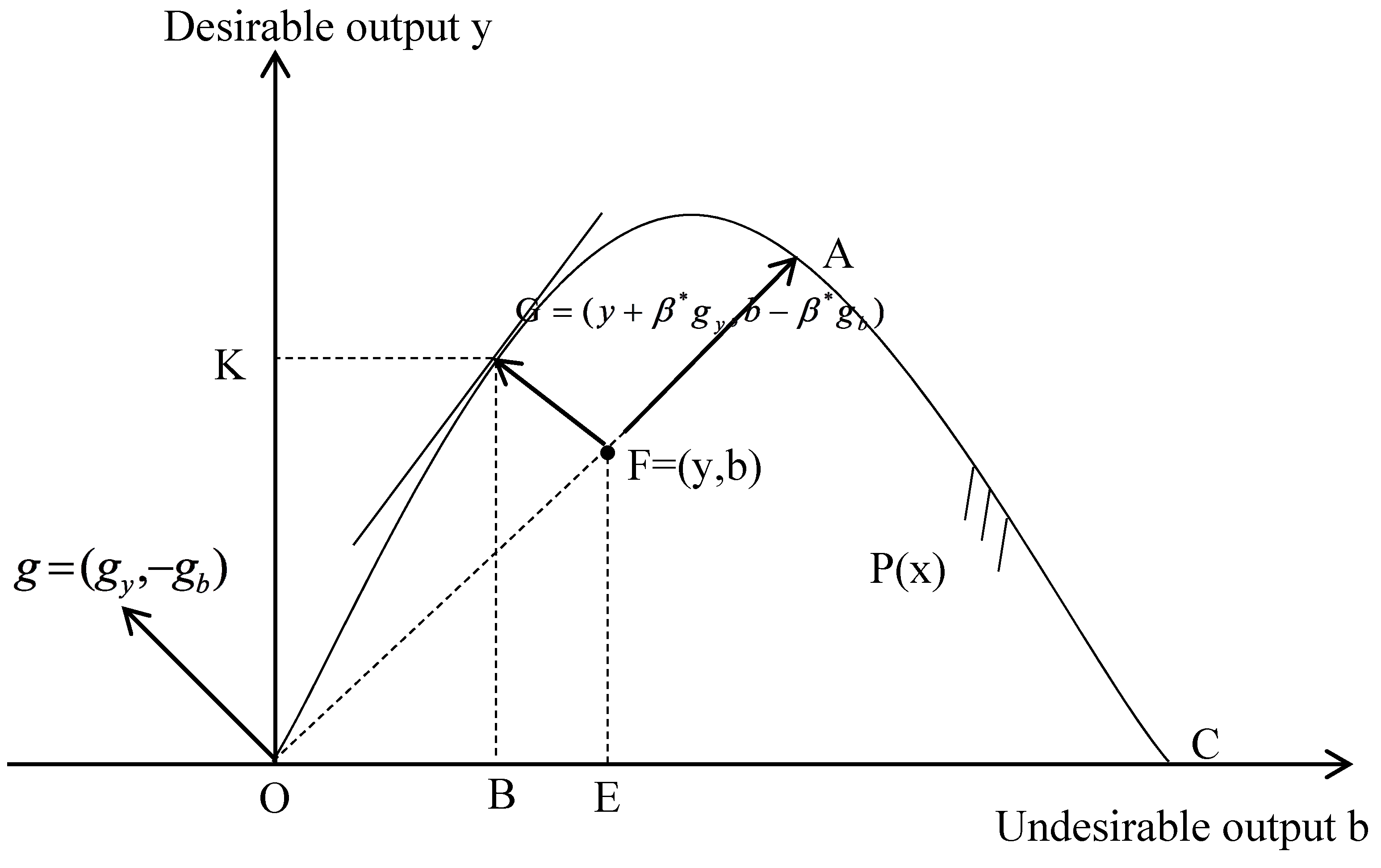
We use Figure 1 to introduce and compare these two functions.

We assume a power plant F is located in the production technology set P(x), which is bound by the curve OAC and the horizontal axis OC, the latter of which is not included due to its null-joint property. The b- and y-axes represent CO₂ and electricity, respectively. A move toward point A could describe the output distance function defined as the ratio of OF and OA, or ${\lambda }^{*}=\mathrm{OF}/OA$. The move toward G by direction vector g could describe the directional distance function. Further, ${\beta }^{*}=\max \beta$ is the maximum capacity to expand desirable outputs and reduce undesirable outputs.

In the production possibility set, the directional distance function is non-negative, and the directional distance function’s value is zero when the output vector (y, b) is on the frontier of P(x).

$$D_0(x,y,b,g)\ge 0\forall (y,b)\in P(x),$$

(7)

If a power plant produces more desirable outputs and the same undesirable outputs with the same inputs, the directional distance function’s value does not increase.

$$D_0(x,y^{\prime },b;g)\le D_0(x,y,b;g)for(y^{\prime },b)\ge (y,b)\in P(x),$$

(8)

If a power plant produces more undesirable outputs and the same desirable outputs with the same inputs, the directional distance function’s value does not increase.

$$D_0(x,y,b^{\prime };g)\ge D_0(x,y,b;g)for(y,b^{\prime })\ge (y,b)\in P(x),$$

(9)

The desirable and undesirable outputs jointly satisfy the property of weak disposability.

$$D_0(x,\theta y,\theta b;g)\ge 0for(y,b)\in P(x)and0\le \theta \le 1,$$

(10)

Another important property for the directional distance function is the translation property.

$$D_0(x,y+\alpha g_y,b-\alpha g_b;g)=D_0(x,y,b;g)-\alpha ,$$

(11)

The directional distance function will be more efficient by the amount of α if the desirable outputs expand αg_y while the undesirable outputs reduce αg_b.

Aigner et al. [20] first established the stochastic frontier function, with the model shown below:

$$\begin{array}{l}y=\beta x+v-u\\ u=\left|U\right|,U\sim N\left[0,{\sigma }_u^2\right],\\ v\sim N\left[0,{\sigma }_v^2\right]\end{array}$$

(12)

where v and u represent the random error and inefficiency, respectively. In practical application, the random error is typically assumed as normally distributed: $v\sim N\left[0,{\sigma }_v^2\right]$, while u is distributed half-normally on the non-negative part of the real number axis: $u=\left|U\right|,U\sim N\left[0,{\sigma }_u^2\right]$.

As the inefficiency value on the production frontier equals zero, we set zero as the dependent variable. If we insert DDF into the SFA model, we obtain the below equation:

$$0=D_0(x,y,b,g)+v-u,$$

(13)

The function’s translog and quadratic form are typically used to calculate the stochastic DDF. The function’s translog form describes a simultaneous change in desirable and undesirable output, while its quadratic form describes the simultaneous desirable outputs’ increase and undesirable outputs’ decrease [11]. Further, the function’s quadratic form could satisfy the DDF translation property. Hence, the function’s quadratic form is suitable for our study:

$$\begin{array}{cc}\hfill D_0(k_{it},l_{it},e_{it},b_{it};g)& ={\beta }_0+{\beta }_k{k}_{it}+{\beta }_e{e}_{it}+{\beta }_y{y}_{it}+{\beta }_c{b}_{it}\hfill \\ & +{\beta }_{kl}{k}_{it}{l}_{it}+{\beta }_{ke}{k}_{it}{e}_{it}+{\beta }_{ky}{k}_{it}{y}_{it}+{\beta }_{kc}{k}_{it}{b}_{it}\hfill \\ & +{\beta }_{le}{l}_{it}{e}_{it}+{\beta }_{ly}{l}_{it}{y}_{it}+{\beta }_{lc}{l}_{it}{b}_{it}+{\beta }_{ey}{e}_{it}{y}_{it}\hfill \\ & +{\beta }_{ec}{e}_{it}{b}_{it}+{\beta }_{yc}{y}_{it}{b}_{it}+\frac{1}{2}{\beta }_{kk}{(k_{it})}^2+\frac{1}{2}{\beta }_{ll}{(l_{it})}^2\hfill \\ & +\frac{1}{2}{\beta }_{ee}{(e_{it})}^2+\frac{1}{2}{\beta }_{yy}{(y_{it})}^2+\frac{1}{2}{\beta }_{cc}{(b_{it})}^2\hfill \end{array},$$

(14)

where y represents the desirable output (electricity) and b represents the undesirable output (CO₂); k, l, and e represent the inputs’ installed capacity, number of employees, and coal consumption, respectively; g represents the direction vector; i = 1, 2, …, N represents each power plant; and t represents each year.

We set the direction vector g = (1,−1) and the undesirable output b as the dependent variable. According the DDF translation property, we can obtain:

$$-b=D_0(k,l,e,y+b,0,1,-1)+v-u,$$

(15)

Equations (14) and (15) allow us to calculate each variable’s values to thus discern the MAC value.

$$\begin{array}{cc}\hfill -b_{it}& ={\beta }_0+{\beta }_k{k}_{it}+{\beta }_l{l}_{it}+{\beta }_e{e}_{it}+{\beta }_y(y_{it}+b_{it})+{\beta }_{kl}{k}_{it}{l}_{it}\hfill \\ & +{\beta }_{ke}{k}_{it}{e}_{it}+{\beta }_{ky}{k}_{it}(y_{it}+b_{it})+{\beta }_{le}{l}_{it}{e}_{it}+{\beta }_{ly}{l}_{it}(y_{it}+b_{it})\hfill \\ & +{\beta }_{ey}{e}_{it}(y_{it}+b_{it})+\frac{1}{2}{\beta }_{kk}{(k_{it})}^2+\frac{1}{2}{\beta }_{ll}{(l_{it})}^2+\frac{1}{2}{\beta }_{ee}{(e_{it})}^2\hfill \\ & +\frac{1}{2}{\beta }_{yy}{(y_{it}+b_{it})}^2+v_{it}-u_{it}\hfill \end{array},$$

(16)

$${\beta }_y-{\beta }_b=-1,{\beta }_{yy}={\beta }_{bb}={\beta }_{yb},{\beta }_{kb}={\beta }_{ky},{\beta }_{lb}={\beta }_{ly},{\beta }_{eb}={\beta }_{ey},$$

According to Fare et al. [6] and Chung et al. [31], the MAC formula is noted as follows:

$$q_{it}=-p_{it}\frac{\partial D_{it}(k_{it},l_{it},e_{it},y_{it},b_{it};1,-1)/\partial b_{it}}{\partial D_{it}(k_{it},l_{it},e_{it},y_{it},b_{it};1,-1)/\partial y_{it}},$$

(17)

where qi represents the MAC value for the undesirable outputs (CO₂), and pi represents the price of the desirable outputs (electricity).

Through substitution and calculation, the final MAC formula can be denoted as:

$$q_{it}=-p_{it}\frac{{\beta }_b+{\beta }_{kb}{k}_{it}+{\beta }_{lb}{l}_{it}+{\beta }_{eb}{e}_{it}+{\beta }_{yb}{y}_{it}+{\beta }_{bb}{b}_{it}}{{\beta }_y+{\beta }_{ky}{k}_{it}+{\beta }_{ly}{l}_{it}+{\beta }_{ey}{e}_{it}+{\beta }_{yb}{b}_{it}+{\beta }_{yy}{y}_{it}},$$

(18)

4. Empirical Results

4.1. Data and Variables

We employ the SFA approach as proposed in Section 3 to examine the efficiency and MAC for Korean coal-fueled power plants from 2008 to 2016. We collected all data regarding 50 major coal-fueled power plants from the Korea Electric Power Corporation’s Statistics of Electric Power (2009–2017). As the output variables, we define each power plant’s gross electricity generation (in kMWh) and carbon dioxide emissions (in KT) as the desirable and undesirable outputs, respectively. However, no carbon dioxide emissions data exists for direct use. Therefore, we follow the criteria published on the website of the International Panel on Climate Change [32] and the NRDC’s National Coordination Committee Office on Climate Change and Energy Research Institute to calculate CO₂ as follows:

$$C{O}_2=E\times CF\times CC\times COF\times \left(44/12\right),$$

(19)

where E indicates the consumed coal; CF indicates the transformation factor, in tons of carbon/TCE; CC indicates the carbon content; and COF indicates the carbon oxidation factor, which measures the percentage of carbon actually oxidized when combustion occurs. The figure “44/12” indicates the ratio of the molecular weight of CO₂ to the molecular weight of carbon. The CF, as reported by the Korean Ministry of Knowledge Economy, is used to estimate CO₂ emissions.

Regarding the inputs, we selected the installed capacity (in MW) as the capital input k, coal consumption (in KT) as the energy input e, and the number of employed staff as the labor input l. As shown in the

Table 2. Descriptive statistics.

Variable	Type	Unit	Mean	Std. Dev.	Max.	Min.
Gross electricity generation	Desirable output	kMWh	3845.453	1307.558	7542.28	645.85
Carbon dioxide emissions	Undesirable output	KT	3033.143	1039.471	6658.7	509.8
Installed capacity	Input	MW	404.7144	138.6494	839.6	72.4
Coal consumption	Input	KT	8465.684	2765.298	16,288	1298
Staff employed	Input	Per Person	296.5129	95.86605	599	72

Source: Korea Electric Power Corporation’s Statistics of Electric Power (2009–2017) (http://epsis.kpx.or.kr/epsisnew/selectEkccIntroEn.do?menuId=110100).

, the input and output data, as well as electricity prices P, are collected from the Korea Electric Power Corporation’s Statistics of Electric Power (2009–2017) [33].

4.2. Empirical results and discussion

Based on Equation (16),

Table 3. Parameter estimates.

Parameter	Coefficient (Std. Err.)	Parameter	Coefficient (Std. Err.)
${\beta }_l$	0.9858931 (0.5876951)	${\beta }_{kk}$	0.0073025 (0.0014773) ***
${\beta }_k$	3.928985 (0.6886737) ***	${\beta }_{ke}$	−0.0011348 (0.0002738) ***
${\beta }_e$	0.0746601 (0.0465364)	${\beta }_{ee}$	0.000076 (8.54 × 10−6) ***
${\beta }_y$	−0.7874651 (0.0658945) ***	${\beta }_{yy}$	−0.0000973 (0.0000529)
${\beta }_{ll}$	−0.0043745 (0.0034043)	${\beta }_{ly}$	0.0006063 (0.0005357)
${\beta }_{kl}$	.0093775 (.0044111) ***	${\beta }_{ky}$	0.0003559 (0.0003895)
${\beta }_{le}$	−0.0008875 (0.0003981) ***	${\beta }_{ey}$	0.0000325 (0.0000228)
${\beta }_0$	−106.3687 (33.3016) ***

Note: The standard deviation is provided in parentheses; *** denotes significance at the 1% level.

displays the all parameter estimate coefficients incorporated into the Stata software program to solve the SFA problem.

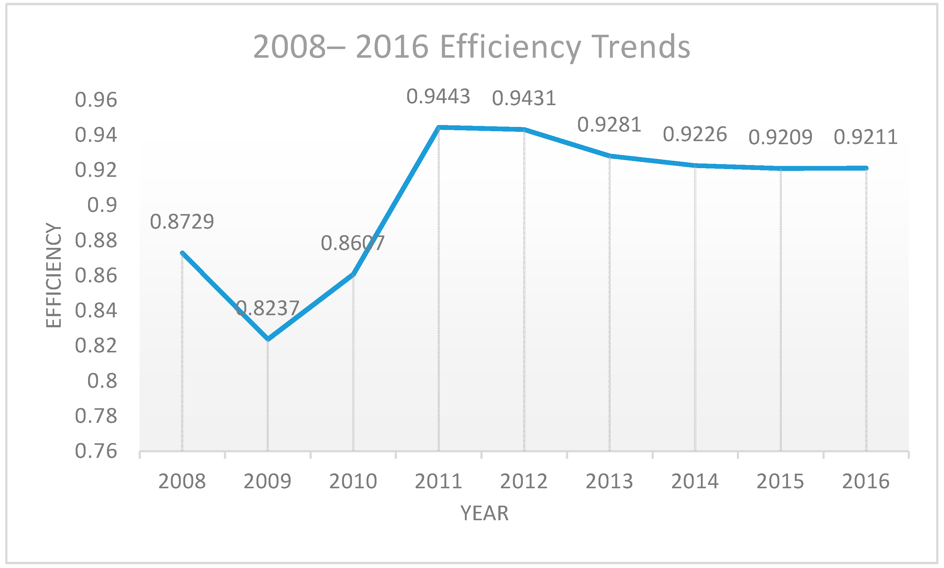
Equation (16) allows us to obtain efficiency results by calculating the inefficient u; Figure 2 illustrates the average efficiency among 50 Korean major coal-fueled power plants from 2008 to 2016. From 2008 to 2012—but except for 2009 when the global financial crisis occurred—Korean coal-fueled power plants’ efficiency exhibits a conspicuous upward trend, from 0.87 to 0.94. This occurred due to the Lee Myung-bak government’s “green economic growth strategy,” which is based on Korea’s domestic and international needs and focuses on long-term development. This strategy parallels Korea’s social reality, in that the country has limited resources. Korea has benefited from this strategy, as it could complete its economic restructuring and quickly recover from this global crisis’ financial abyss.

From 2013 to 2016, the efficiency of Korea’s coal-fueled power plants displays no improvement, but rather, a slight decline. This is because President Park Geun-hye came into power with a three-year plan for economic reform, modeled after President Park Chung-hee’s five-year plan for economic development. The latter plan established a goal of increasing the nation’s potential growth rate by more than 4 percent, increasing the employment rate to 70 percent, and increasing the annual national income to $40,000 per capita. The more recent three-year plan for economic reform excessively emphasized rapid economic growth, with too little emphasis on efficient, green, and sustainable development. This economic policy sacrifices economic development quality for speed.

Korea launched its ETS in 2015, but we found that from 2015 to 2016, the carbon market did not positively impact the efficiency of coal-fueled power plants, which are major players in the carbon market. Therefore, we will explore why this occurred from a MAC perspective.

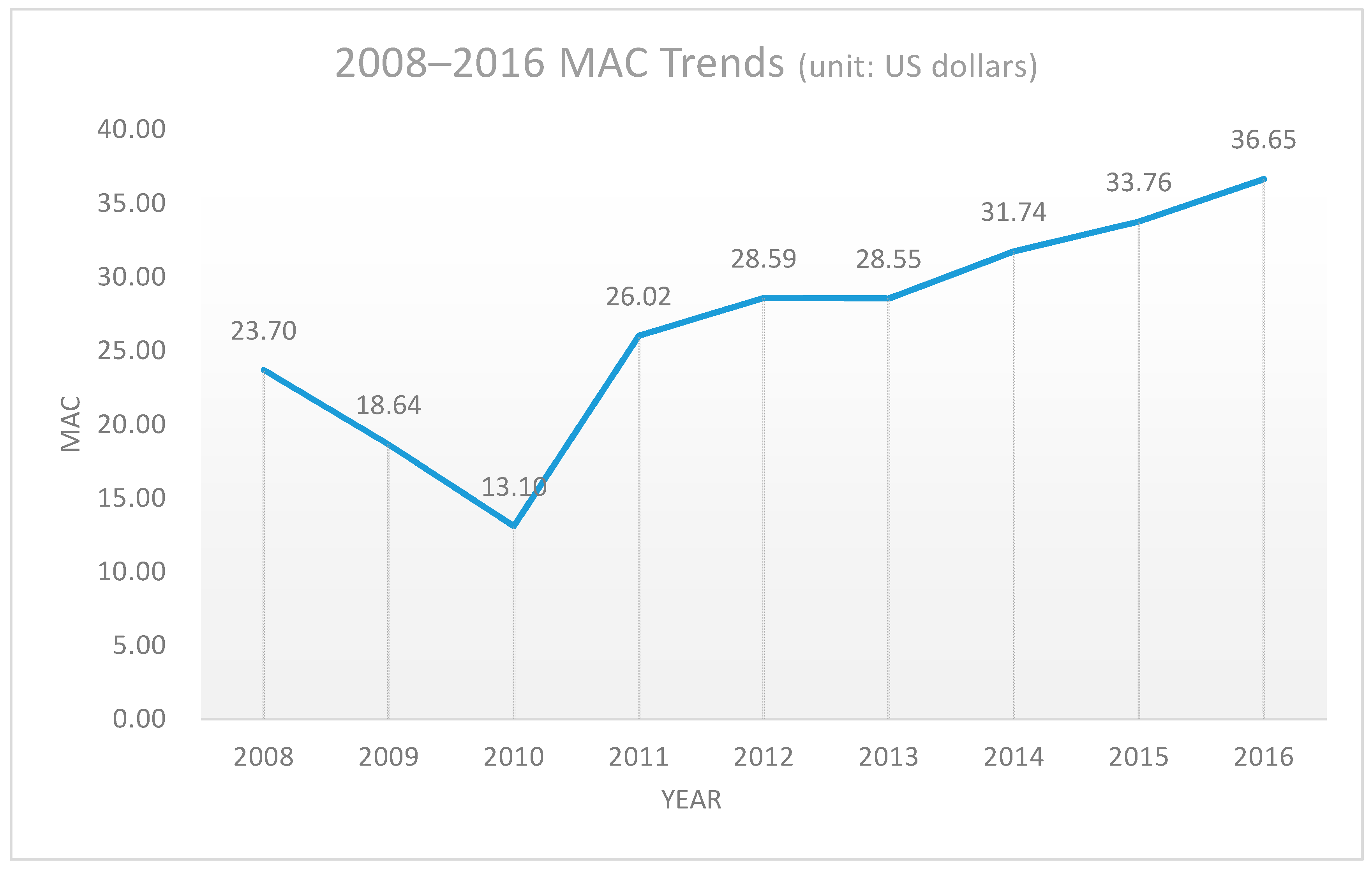
Figure 3 illustrates the average MAC for Korea’s 50 major coal-fueled power plants from 2008 to 2016. This not only presents an estimated value of the opportunity cost for undesirable output, but also provides meaningful guidelines for such output to formulate regulatory policies for public decision-makers [29].

Table 4. Previous studies’ results regarding Korean coal-fueled power plants.

Previous Study (Year of Publication)	Time	Measure	Average CO2 MAC (in US dollars)
Kwon and Yun (1999)	1990–1995	SDF	3.34
Park and Lim (2009)	2001–2004	SDF	15.77
Lee (2011)	2007	SDF	14.63

provides previous studies’ MAC values for Korean coal-fueled power plants. The estimation results for CO₂ MAC differ because of the authors’ different methods, datasets, and sample periods. However, all of these papers used the Shepard distance function (SDF), which is characterized by its parameter flexibility, and which has been widely used in estimating pollutants’ shadow pricing. This function assumes that both desirable and undesirable outputs simultaneously increase or decrease, implying a lower MAC estimation due to this type of simultaneous buffer. Moreover, these estimated values are based on the non-regulatory regime, and consequently, do not appropriately reflect MAC values.

Compared with these values, our resulting MAC estimates are higher than in previous studies, as we consider random errors and statistical noise. Moreover, our estimated values are based on the realized regulatory regime, implying utmost pressure for additional production with much higher opportunity costs in terms of MAC.

We converted the price into US dollars at each year’s exchange rate for a more convenient comparison. According to our MAC results, Korean coal-fueled power plants’ MAC dramatically decreased from 2008 to 2019, but rapidly recovered in 2011. At this time, the MAC recovered to a rate of approximately 26 dollars, then exhibited a gentle growth from 2011 to 2016 due to increasing electricity prices, as it increased to a rate of 10 dollars during the five-year period. After the Korean ETS was established, Korean coal-fueled power plants’ MAC were 33.76 and 36.65 dollars in 2015 and 2016, respectively.

Table 5. The Korean ETS’ 2015–2016 trading volume (in thousands/ton).

	2015				2016
	Q1	Q2	Q3	Q4	Q1	Q2	Q3	Q4
KAU	1			398	102	1647	1184	551
KCU		780		141	613	1408	100	59
KOC		1130	1913	1371	2294	1526	663	1113
Total	1	1910	1913	1910	3008	4581	1946	1723

Source: Korea Ministry of Environment (2017).

displays the Korean ETS’ trading volume in 2015 and 2016, with KAU signifying the Korean allowance unit, KCU the Korean credit unit, and KOC the Korean offset credit. Although the 2016 trading volume increased by 96.27% compared with that in 2015, the trading volume accounted for a miniscule proportion of the total quota in the Korean ETS market. The 2015 trading volume accounted for 0.8% of the total quota, while the 2016 trading volume accounted for 1.6%. The market’s lack of participants has prevented it from functioning as it should.

Table 6. The Korean ETS’ 2015–2016 market price (in US dollars/ton).

	2015				2016
	Q1	Q2	Q3	Q4	Q1	Q2	Q3	Q4
KAU	7.38			10.54	15.11	15.29	14.85	16.08
KCU		9.05		12.48	14.59	16.26	15.64	16.26
KOC						16.26	15.82	15.99
Average	7.38	9.05		11.16	14.59	15.82	15.11	16.08

Source: Korea Ministry of Environment (2017).

notes the Korean ETS’ market price in 2015 and 2016. We converted the price into US dollars at each year’s exchange rate for a more convenient comparison. As this table indicates, the second quarter has a relatively heavy trade volume and higher prices, as all the member companies report their quotas’ fulfillment each June; this implies that the market heavily depends on regulatory policies. This table demonstrates that the real market price is much lower than our MAC result; in other words, the market price reflected just 27.24% and 42.02% in 2015 and 2016. This situation indicates that the ETS market price is too low to encourage coal-fueled power plants to actively participate in the carbon emissions-trading market. The extraordinarily low market price leads to less supply from the power plants, and thus, no quota exists for power plants that need higher quotas to purchase. Subsequently, their quotas include too little supply relative to too much demand. Their small trading volume also supports the fact that low carbon prices prevent the ETS’ proactive operation. Therefore, the ETS markets cannot function well to achieve their objectives.

5. Conclusions

Korea is the world’s 11th largest economy, a major energy consumer, and the world’s seventh-largest producer of carbon dioxide emissions, with 679.7 million tons of CO₂ produced in 2017. In the same year, Korea accounted for 2.3% of total global coal consumption. To improve economic efficiency and protect the natural environment, the Korean government committed to the 2015 Paris Agreement by deciding to reduce GHG emissions by 37% from BAU levels by 2030. Korea’s government launched its national ETS in 2015 to achieve this target.

The environmental efficiency results from Korean coal-fueled power plants revealed that rapid growth occurred under Lee Myung-bak’s government, except in 2009 during the global financial crisis. This result demonstrates the benefits from Lee Myung-bak’s “green economic growth” government strategy, which formulated detailed policies for sustainable development. However, efficiency results exhibited a slight downward trend under Park Geun-hye’s government. This occurred because the latter government’s economic policies excessively emphasized rapid economic development and neglected long-term sustainable development. This government changed its quota from 97% to 100% allowances, implying that companies had no obligation to reduce its emissions unless it produced more than the average of the three previous years. This loosened regulation deterred companies from reducing their emissions, and the government’s price regulations in the market were too low for the companies to “sell” their performance on the market. Consequently, the economy became a seller’s market, without any seller voluntarily reducing their emission allowances, and the coal-fueled power industry was not an exception to this phenomenon. Therefore, the Korean government should again prioritize green development in its economic development policies to promote high-quality sustainable development, instead of establishing excessive, unrealistic economic development targets that negatively affect efficient economic development as well as the natural environment.

This study also discovered a substantial gap between carbon market prices and our MAC results, which makes the market’s healthy functioning impossible to help increase coal-fueled power plants’ efficiency. Thus, policymakers should impose a carbon tax, adjust their carbon emissions quotas, and introduce more regulatory measures—and especially for coal-fueled power plants—to fill gaps of 57.98% in 2015 and 72.76% in 2016. This will maintain market prices within a reasonable range and correct the serious imbalance between supply and demand. The market can then play an important role in improving coal-fueled power plants’ efficiency by saving energy while reducing emissions. Further, policymakers should reduce carbon transaction costs in the ETS market and encourage power plants to more actively participate in trading activities.

However, this study ignored the influence of the “Management of Targets for GHGs and Energy” system’s influence on the ETS. Future studies should not perceive the ETS as an isolated institution, but should consider the impacts from this management system.