The Eco-Costs of Material Scarcity, a Resource Indicator for LCA, Derived from a Statistical Analysis on Excessive Price Peaks

Abstract

The availability of resources is crucial for the socio-economic stability of our society. For more than two decades, there was a debate on how to structure this issue within the context of life-Cycle assessment (LCA). The classical approach with LCA is to describe “scarcity” for future generations (100–1000 years) in terms of absolute depletion. The problem, however, is that the long-term availability is simply not known (within a factor of 100–1000). Outside the LCA community, the short-term supply risks (10–30 years) were predicted, resulting in the list of critical raw materials (CRM) of the European Union (EU), and the British risk list. The methodology used, however, cannot easily be transposed and applied into LCA calculations. This paper presents a new approach to the issue of short-term material supply shortages, based on subsequent sudden price jumps, which can lead to socio-economic instability. The basic approach is that each resource is characterized by its own specific supply chain with its specific price volatility. The eco-costs of material scarcity are derived from the so-called value at risk (VAR), a well-known statistical risk indicator in the financial world. This paper provides a list of indicators for 42 metals. An advantage of the system is that it is directly related to business risks, and is relatively easy to understand. A disadvantage is that “statistics of the past” might not be replicated in the future (e.g., when changing from structural oversupply to overdemand, or vice versa, which appeared an issue for two companion metals over the last 30 years). Further research is recommended to improve the statistics.

1. Introduction

1.1. Resource Scarcity in the Classic Environmental Life-Cycle Assessment (LCA)

The availability of resources is crucial in our modern society from a socio-economic point of view. It is one of the main drivers behind the new “circular business models” for companies, and the “circular economy” at the level of countries. Thus, availability is high on the agenda in the United States of America (USA), as well as in the European Union (EU), leading to comprehensive studies and datasets of the British Geological Survey [1], the United States Geological Survey (USGS) [2], and the European Commission [3]. The main risk is a sudden disruption of the supply chain because of, for example, (geo)political unrest, causing an unexpected major price jump. Resources which have such a risk, and which are important for our economy, are termed “critical”. The issue is here the short-term availability for current generations (10–30 years).

In the classic environmental LCA, however, the focus is always on the long-term (absolute) depletion of materials [4]; materials must be preserved for future generations, i.e., 100–1000 years. The issue is then the ratio of the mineral resources in the earth’ crust, and deaccumulation of that mineral, which resulted in the development of the abiotic depletion potential (ADP) [5,6,7,8].

ADP = (D/R²)/(D_ref/R_ref²),

(1)

where ADP is the abiotic depletion potential, R is the ultimate reserve of a resource in the earth crust (kg), D is the deaccumulation of that metal reserve (kg/year), R_ref is the ultimate reserve of antimony as a reference metal (kg), and D_ref is the deaccumulation of antimony as a reference metal (kg/year).

The ADP is the most applied indicator for resource depletion in LCA practice. The ADP is, however, not without problems. The denominator, R, is extremely uncertain (even more uncertain than the long-term deaccumulation estimate, D), and it is squared as well, enlarging the uncertainty problem. Greadel et al. [9] studied the availability in depth for a number of metals. They concluded that the available amount is simply not known, whether as an absolute value or as a ratio between the metals. The reason is the distinct different mining situations in practice such as the type of host rock, the distribution of the grade in the deposit, and the issue of co-mining. Greadel et al. compared the extractable global resource (EGR) with the reserve base (RB) estimates of the USGS. They calculated a variance of a factor of 100 for the EGR/RB ratio from a list of 64 metals, (eight had more than a factor of 800). The tectonic diffusion estimates [10] are an order of magnitude higher.

The real issues, however, are (1) the uncertainty in new discoveries through exploration [11,12], and (2) reduction of primary mining because of increasing recycling rates and replacement of metals by other materials in products (substitution) [13,14]. Most environmentalists take the ultimate extractable reserves as a calculation basis; they seem to ignore the two issues above, and adhere to a fixed-stock paradigm as a precautionary principle. Experts in the mining industry report a much more optimistic perspective [15,16]. In general, one may conclude that it is hard to make any reliable forecast for the depletion of metals over the coming 100–1000 years. The uncertainties are much too high.

There are other approaches to the issue of metal depletion in LCA, inspired by an early publication on (metal) resources and energy, dealing with resource depletion [17]. This publication deals with the issue that metals are widely available in the earth crust; however, the limiting factor is the energy (and, hence, the cost) to allow these lower-grade ores to be mined and refined [18,19]. The fixed-stock paradigm leads to ever-increasing prices for future generations. The most applied method in LCA along this line of thinking is the ReCiPe method [20,21,22]. The problem with this approach, according to experts in the mining industry, is “that grades have so far been of limited relevance to the issue of availability” ([16], Section 10). There are many different arguments for this statement (see also an analysis on this issue [23]).

The eco-costs 2007 model [24] was also based on the idea of a fixed stock with ever-increasing prices, but that idea was abandoned after an analysis of price trends over the period 1900–2013 of 35 metals by Henckens [13], showing that average prices (corrected for inflation) remained fairly constant over these 11 decades. Even the average trend in copper prices declined as a rate of 3% every 10 years since 1900 (before 1900, the prices were even higher), despite ever-decreasing ore grades (see Figure 1). Thus, there is no evidence for approaches which are based on long-term rising costs. Copper shows in the same time span, however, heavy price volatility, which underlines the need for indicators based on these short-term price fluctuations.

Many LCA scientists seem to accept the aforementioned long-term uncertainties as a fact of life, and still apply midpoint tables that are based on the absolute depletion of resources (see

Table 1. Resource evaluation of some leading indicator systems in life-cycle assessment (LCA). Abbreviations: CML= Centrum voor Milieuwetenschappen, EPS = Environmental Priority Strategies, EDIP = Environmental Development of Industrial Products, EPD = Environmental Product Declaration, ILCD = International Life Cycle Data, ADP = Abiotic Depletion Potential, AADP = anthropogenic stock extended abiotic depletion potential, MJ = Mega Joule, UBP = Umweltbelastungspunkte, ELU = Environmental Load Units, PR = person-reserves.

Method	Indicator	Approach	Fixed-Stock Paradigm?	Reference
CML-1	ADP	Equation (1)	Yes	[5,6,7]
Anthropogenic stock extended ADP model	AADP	Equation (1), including anthropogenic stock	Yes	[8]
Eco-indicator 99	MJ surplus	Extra energy required	Yes	[20]
ReCiPe 2008	US$	Surplus cost mining	Yes	[21]
ReCiPe 2016	US$	Surplus cost mining	Yes	[22]
Eco-costs 2007	euro	Surplus cost mining	Yes	[24,25]
Ecological Scarcity 2013	UBP (ADP)	Equation (1)	Yes	[26]
EPS 2015	ELU (euro)	Replacement	No	[27]
EDIP 2003	PR	Time of depletion	Yes	[28]
EPD 2013 (EN15804)	ADP	Equation (1)	Yes	[29]
ILCD 2011 Midpoint+	ADP	Equation (1)	Yes	[30]
IMPACT 2002+	MJ surplus	Extra energy required	Yes	[31]
Eco-costs 2017	euro	Short term scarcity	No	This paper

for some leading indicator systems).

There is, however, a growing number of publications that tried developing alternative indicator systems for scarcity, based on current, short-term observations. Two new short-term approaches can be distinguished: (1) developments outside of LCA that try to characterize the issue of short-term availability by applying a supply risk indicator [1,2,3], as analyzed in Reference [32], and (2) developments that try to broaden the classic environmental LCA approach to LCSA (life-cycle sustainability assessment), adding aspects of S-LCA (social life-cycle assessment) [33,34,35]. Section 1.2 and Section 1.3 of this paper deal with these two approaches. Section 1.4 deals with the knowledge gap in LCA and with the research questions of this paper.

1.2. Metrics on Criticality outside the LCA Community

Achzet and Helbig [36] analyzed 15 criticality methods (published in the period 2006–2011) with regard to the driving factors for instabilities in the supply chain. A total of 20 indicators were found, of which 10 are supposed to be the general driving factors of the supply risk: (1) country concentration, (2) country political risk, (3) depletion time of stocks and reservoirs, (4) by-product dependency, (5) concentration of mining and refining companies, (6) sudden growth of demand, (7) recyclability and recycling potential, (8) substitutability, (9) import dependence, and (10) commodity prices. An interesting observation here, from an economic point of view, is that the commodity prices (number 10 in this list) is not a root cause for a shortage in the supply chain, like the other indicators, but is as a result of the other nine issues that cause the supply shortages (via price elasticity). Achzet and Helbig conclude that aggregation of these indicators is, and remains, problematic as highlighted in the following quotes: (1) “in the real world, raw material risk patterns are of course highly dynamic and vary from element to element”; (2) “empiric evidence about the influence of the indicators on supply risk is missing”.

An ad hoc working group of the European Commission [3] tried, nevertheless, to “predict” the chance of shortages in the supply chain of 41 metals using a complex non-linear formula [37], applying the following four main indicators:

• Concentration of metal-producing countries, applying the Herfindahl–Hirschman index;
• Political stability of producing countries, using the worldwide governance indicators;
• Potential substitution, estimated by expert opinion;
• Recycling rate, from UNEP [38].

This system might be valuable for political decision taking, especially since the end result of the calculation system is a simple yes/no on the question whether a metal is considered in the EU as a CRM (critical raw material). However, such a non-linear formula with threshold values cannot be used in a linear calculation system like LCA [39].

1.3. The Issue of “Resources” in LCA and the Next Step toward LCSA

The first innovative step in LCA, with regard to resource scarcity, was a publication by Schneider et al. [33] on the economic resource scarcity potential (ESP), which is a new model for the assessment of “resource provision capability” for human welfare, from an economic angle. The system has a list of indicators which is quite similar to the aforementioned list in Reference [36] (see Section 1.2). The comparison of this midpoint system with ADP reveals that “the model developed in this work allows for a more realistic assessment of resource availability”. The midpoint indicators, as such, are not expressed in terms of money.

These kinds of developments triggered two discussions: (1) can it be allowed that LCA incorporates socio-economic aspects (the role of resources in human welfare by the functions they provide)? (2) If so, does LCA need expanding to include S-LCA (social life-cycle assessment), to incorporate issues like human rights violations, child labor, and extreme poverty? A working group of the Joint Research Center of the EU concluded that both questions should positively be approached [34].

Sonneman et al. [35] also concluded that the focus on LCA must be broadened to LCSA (incorporating the social aspects of S-LCA): “The socio-economic and geopolitical issues related to natural resources are relevant for sustainability and, hence, need to be an integral part of LCSA if we want to keep the overall LCA methodology appropriate”. The approach of Sonneman is very promising for midpoint-type hotspot analyses. Aggregation of the midpoint scores to one endpoint score, however, is required for LCA benchmarking [40] (see also Figure 8); such a system enables the integration of environmental and social midpoints.

1.4. Research Questions Related to the Development of a New Socio-Economic Approach

It may be concluded from the previous sections that there is still a gap between the developments in LCA and the practical needs in LCA benchmarking, i.e., a single indicator for short-term material scarcity. The development of the CRM quantification metrics in the EU did not lead to a single indicator which can be applied in LCA. One of the problems of the approaches so far is the complex relationship between the different root causes of shortages in the supply chain, as explained in the first paragraph of Section 1.2. Another problem is the variety of definitions which are given to “scarcity” [39]. Since it is evident that the socio-economic issues play a major role in the supply risk evaluation [3,4,33,37], it is a logical next step to look at approaches that are applied in economic sciences on price elasticity and price volatility.

In this paper, such an approach is followed, based on the value at risk (VAR) statistical method, which is widely applied in finance. It is used to analyze the short-term (10–30 years) supply chain risks for our current generations, as described in Section 2.1. This approach is based on statistics of available data on metal prices for several decades in history (enabling VAR calculations starting from 1946).

The research questions are as follows:

(a)

Which statistical method can be applied to predict the future risk of a sudden jump in prices caused by disruptions in the supply chain?

(b)

For which metals are these price fluctuations relevant (i.e., are the price peaks high in comparison to the average price over a decade)?

(c)

How can this approach of supply chain risks and consequential price jumps be incorporated in LCA?

2. Methods and Data

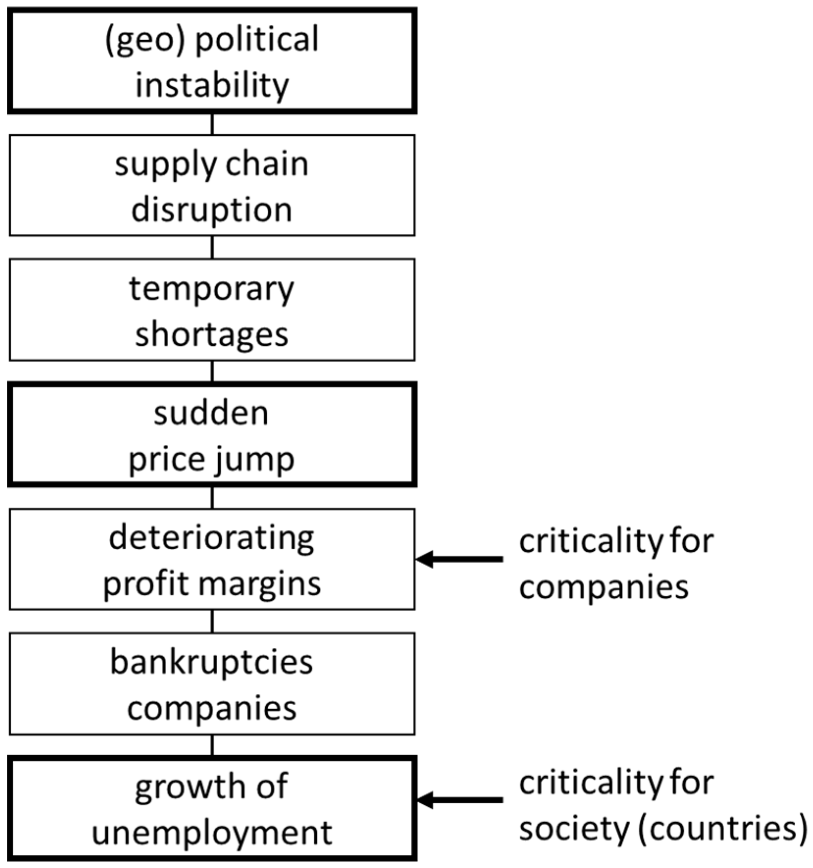
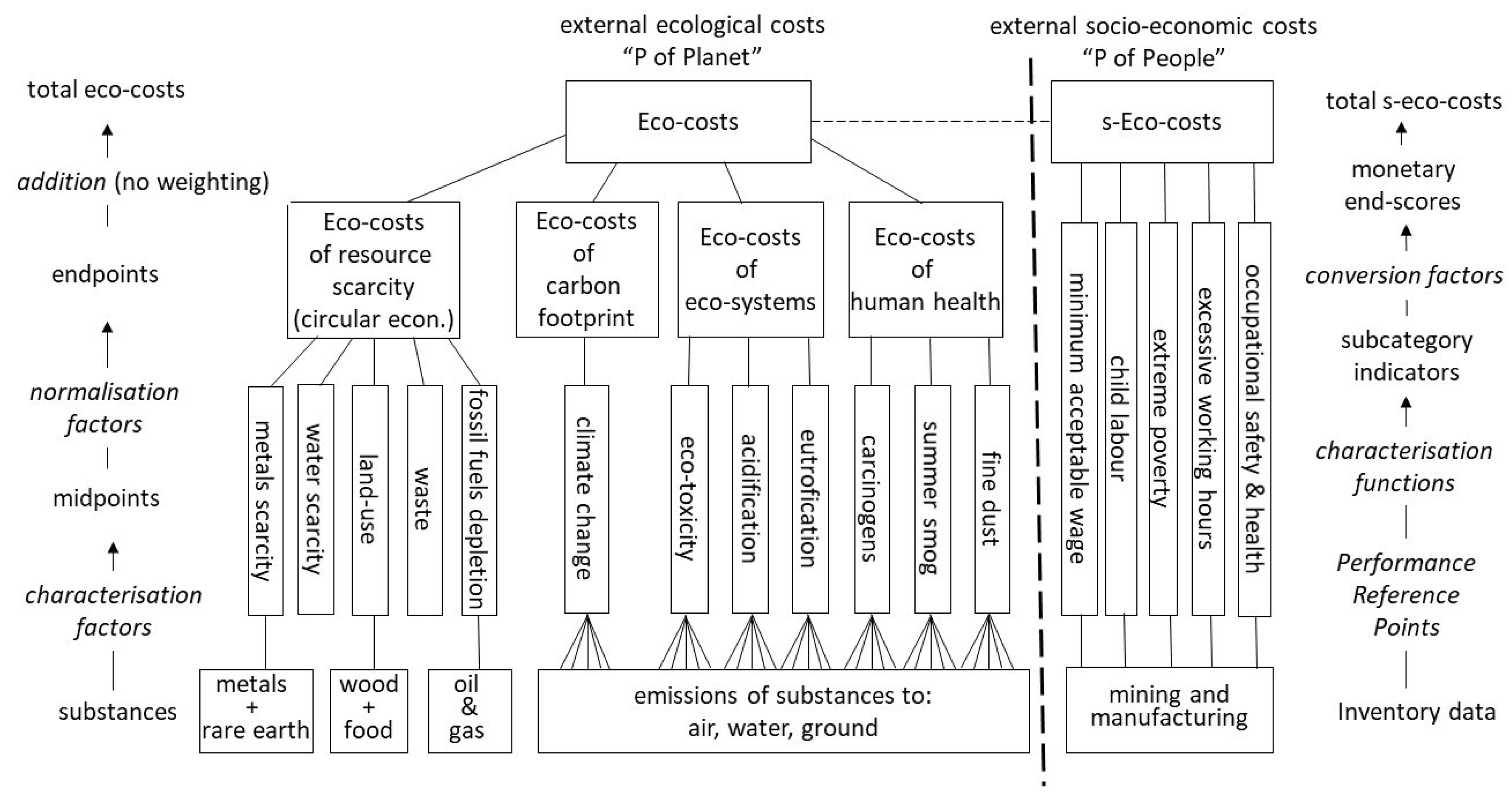
2.1. The Cause–Effect Pathway of the Socio-Economic Effects of Resource Scarcity

The cause–effect pathway of the socio-economic effects of resource scarcity is depicted in Figure 2. It starts with a (geo)political event (e.g., protectionism, social unrest in mining countries, strikes, etc.), which results in supply chain disruptions, or a sudden technical breakthrough. Because of limited stocks in the logistics chain, this will lead to shortages of the material(s). In the free market economy, that will result in higher prices, rising very rapidly, since all market players try to buy material stocks that are available. Companies which need the material will see risks to their profit margins because they cannot quickly increase the sale prices without losing market share. The weakest companies can go bankrupt, resulting in unemployment. That means that this phenomenon results in threats to society [41,42].

This phenomenon is relevant for every manufacturer that purchases metals, but it is also relevant on the level of a country or region. The difference between a company and a country is that a company can suffer from a price jump of every material that has a high proportion of the total purchasing volume (in financial terms), whereas a country might only be interested in materials that are imported in larger volumes and, therefore, have an impact on the gross domestic product (GDP). That is the reason why the EU is mainly interested in what it calls critical raw materials (CRM), i.e., materials that combine a high supply risk with economic importance on the level of the EU member states.

The pathways from the (geo)political unrest to the price jump are extremely complex and context-dependent. A common factor in past price jumps is that they can rarely be predicted 24 or even 12 months before they happen [43]. In the financial world, such discontinuities are called “black swan events” [44,45]: unexpected disruptions with major consequences. The pathway from the price jump to growing unemployment is also extremely complex. This means that there is the situation that the pathway is undoubtedly present, but that it cannot be calculated, which requires a different technique and paradigm than that usually applied in LCA.

The issue here is to predict the risk of a price jump of a certain size in the relatively temporal period of 10 to 30 years. This can be done by statistics, since each metal is characterized by its own volatility in price as a result of its specific supply chain and its specific risks of geopolitical instabilities or quantum leaps in technical demand. Section 2.2 explains that the so-called value at risk at the 95% level on a yearly basis (95% VAR) is a good indicator for such a risk. The 95% VAR indicates the size of a price jump which is only surpassed in 5% of cases in a row of prices. Since prices are dynamic in the longer term as well, the 95% VAR is compared to the 10-year moving average (MA) price. We call this the price peak ratio (PPR; see Figure 3).

PPR = 95% VAR/10-year MA,

(2)

where PPR is the price peak ratio, 95% VAR is the value at risk at the 95th percentile, over yearly prices from 1946–2015 ($ or euro 2015), and 10-year MA is the simple moving average of the price over the last 10 years ($ or euro 2015).

An example of the business risk of such price jumps is given in Appendix A for the hypothetical case of a manufacturer of lithium-ion car batteries.

It is preferable to have products with stable prices (a low PPR) especially in business, which is relevant for the material selection at the design stage of a product. When a material with a high PPR cannot be avoided, circular business models (e.g., reuse, recycling, etc.) can mitigate the supply chain problem.

Since the VAR is a future socio-economic risk, it can fulfil the requirements of an indicator in LCA, especially in the system of the eco-costs in 2017: the 95% VAR = “eco-costs of metal scarcity”, as explained in Section 3.2.

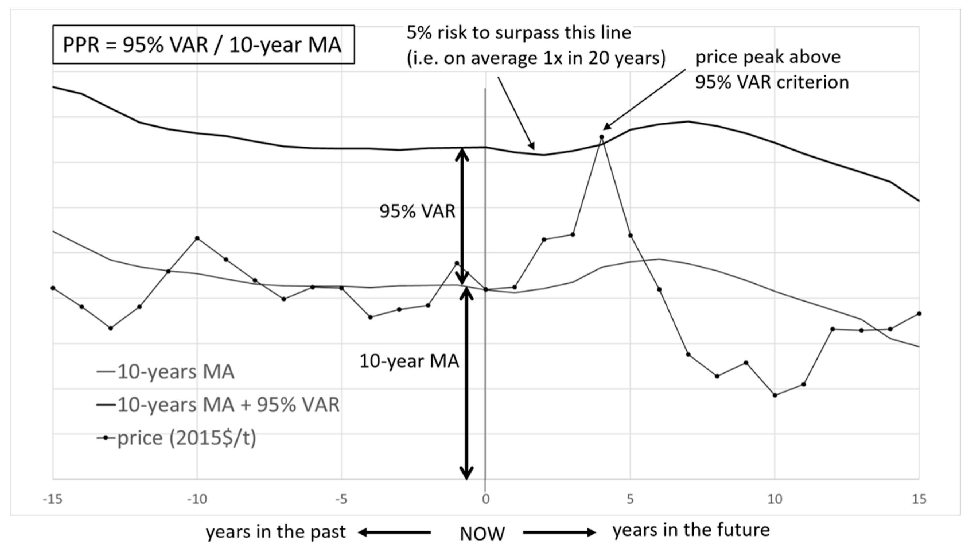
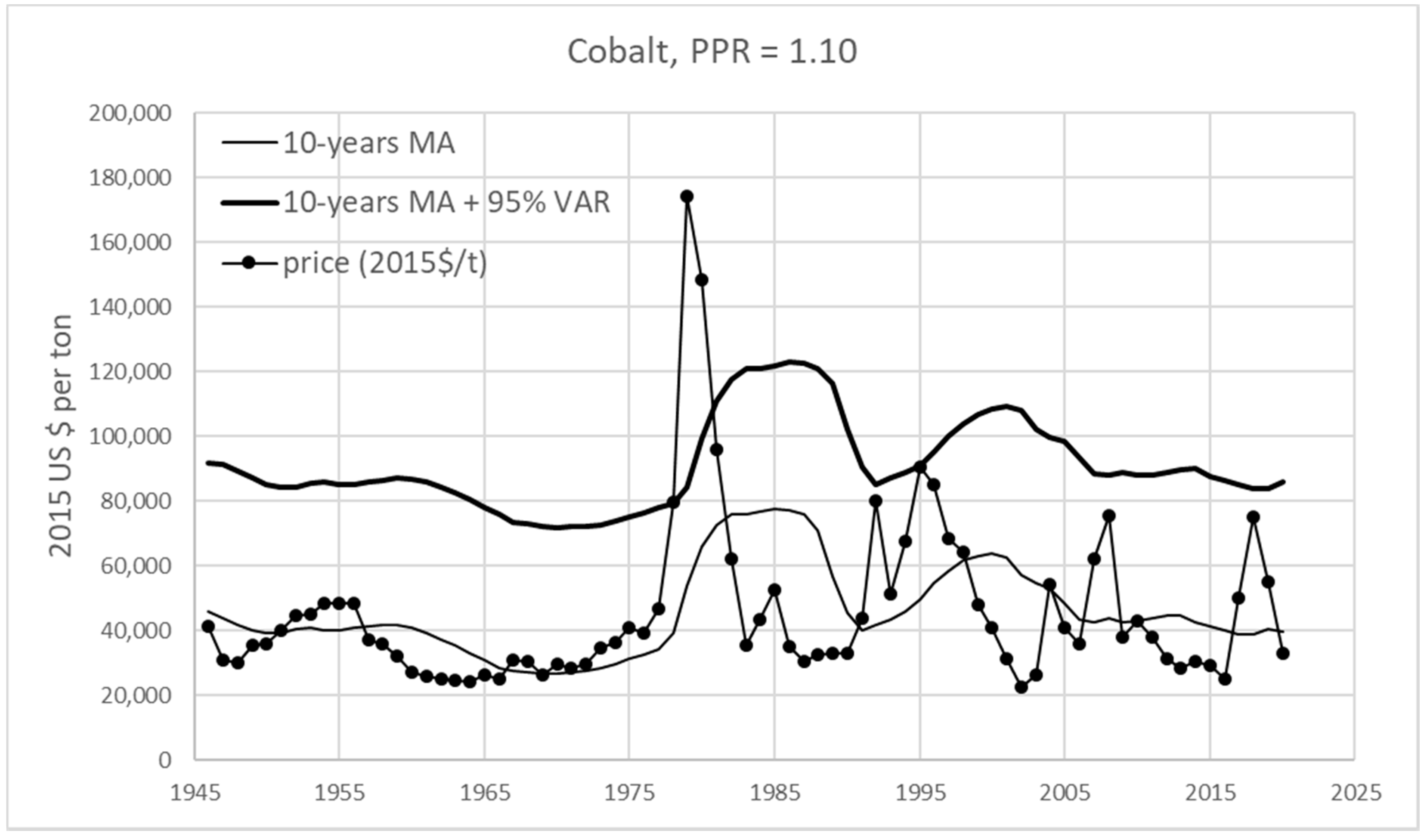
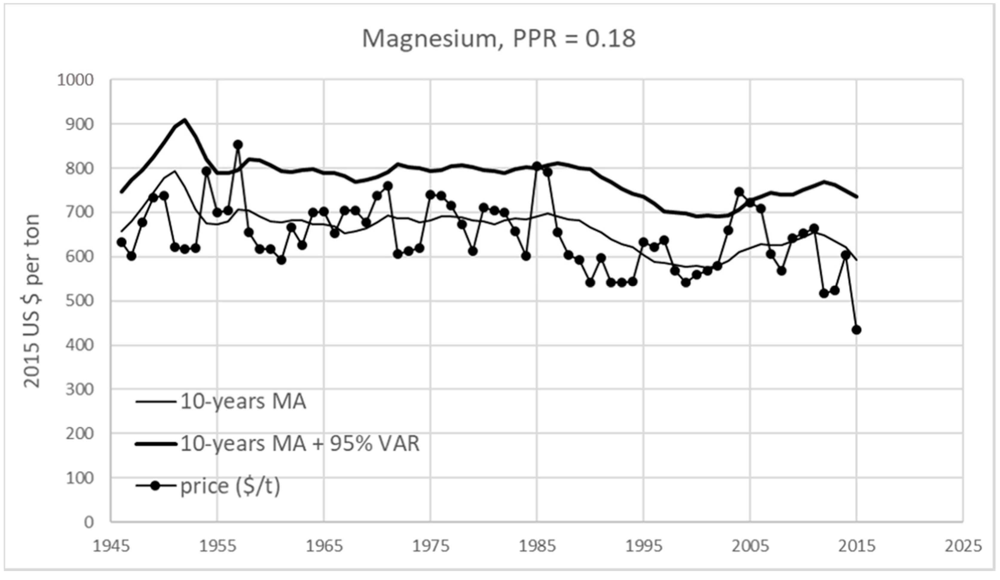
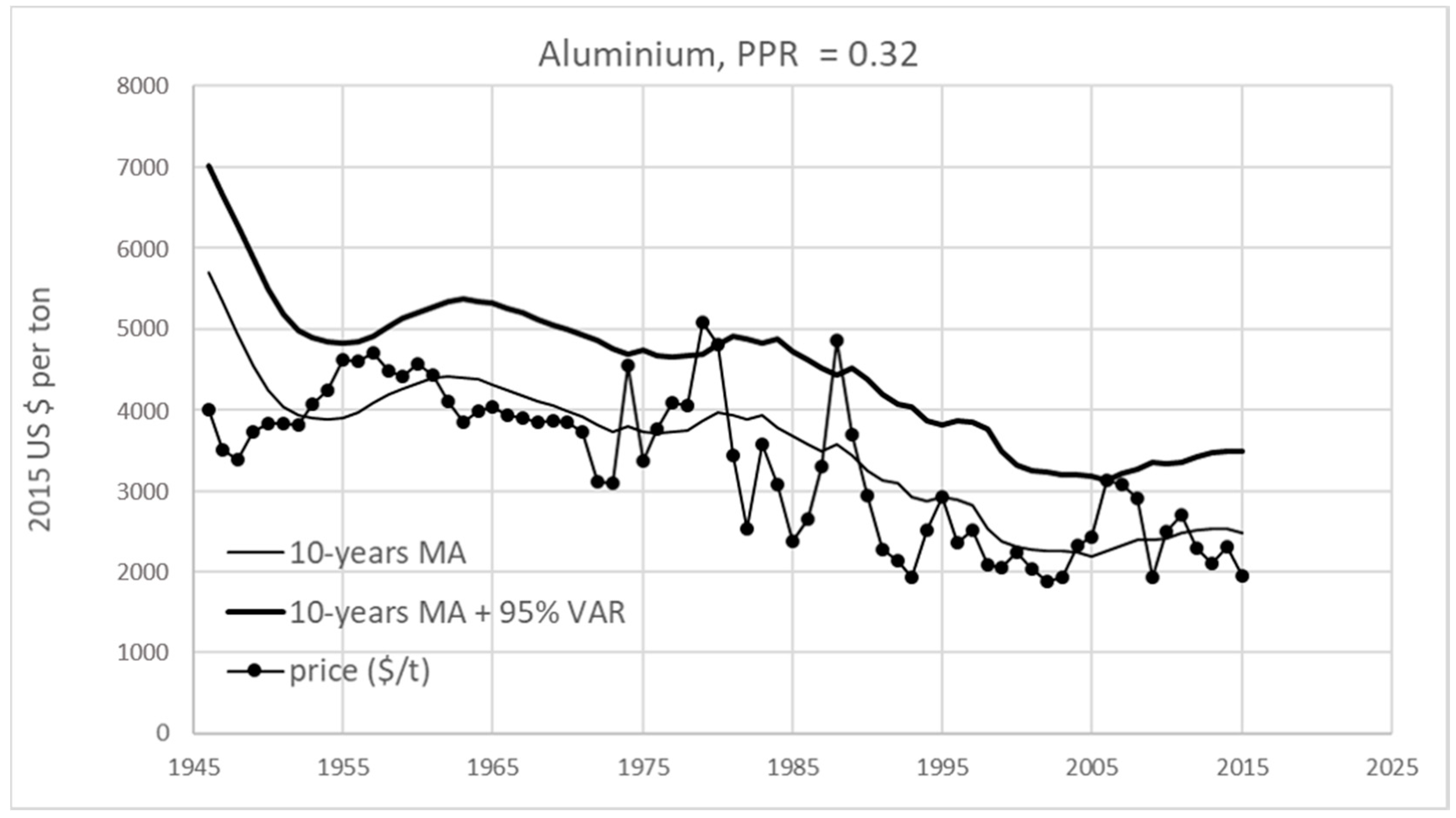
2.2. Quantifying the Risk of Price Fluctuations: The 95% Value at Risk (95% VAR)

The VAR (value at risk) is a popular financial instrument that indicates the fluctuation of the value of an asset. Normally, it is applied to risks with financial assets (e.g., shares, bonds), insurance risks, risks of fluctuating exchange rates, or commodity prices.

The (1 − p) VAR (expressed in euro, US dollar, or any other currency) indicates the fluctuation of the value of an asset, over a certain time period, which can be larger than the value VAR, with a probability p. Common values for p are 5% and 1%. In our study, we apply the maximum price in a time period of one year, with p = 5%. We base our VAR calculation on a dataset of 70 years: prices for the years 1946–2015. Since the calculation requires a moving average of 10 years, the data for the total calculation start 10 years earlier, in 1936. This can be done because of two reasons: (1) the calculation is not very sensitive for the 10-year MA, and (2) there were hardly any excessive price peaks in the period 1946–1956, as can be seen in the Supplementary Materials [46]. A validation check on shifting the start of the calculation from 1946 to 1956 (first year of the 10-year MA is 1936) revealed a small reduction of the VAR (eco-costs) for only four of the 42 metals: beryllium (−20%), cadmium (−22%), silicon (−2%), and tungsten (−14%). It was decided to base the VAR calculation starting at 1946, provided that data were available. When data were only available as of a later year, the start date was adjusted (see Supplementary Materials) [46]. When the USGS publishes a new report with later data, e.g., to the year 2020, the VAR will be recalculated, still starting from 1946. Theoretically this will result in a higher accuracy of the VAR (since it is based on more data). It is expected that the VAR of most of the metals will hardly change, since prices stabilized in the period 2015–2020, apart from a heavy price peak of lithium.

The (1 − p) VAR is a (1 − p)-quantile of distribution of X and, therefore, can be (1) calculated analytically when the distribution of X is known, (2) estimated via Monte Carlo simulation, or (3) estimated non-parametrically via an empirical quantile. Since the distributions of yearly fluctuations of metal prices are not known, 95% VAR was estimated by taking the empirical 95% quantile of the difference of the historical price and the 10-year moving average.

For the calculation of the PPR, the VAR was looked at for the price jumps (see Figure 3); thus, the price peaks were compared to the average price (note that this is a bit different from a VAR in finance, where the VAR is taken of the price itself). The 10-year moving average was taken for three reasons: (1) the current business practice in product innovation takes a maximum of five to 10 years for an average price estimate; (2) experiments showed that averages over more than 10 years do not give significant differences, and averages shorter than five years show less favorable results (see validation check in Section 4.2); (3) an extreme long average over the full 70 years, i.e., the whole data row, would not cope with the multi-year “pig cycles” which are common in metal prices.

The disadvantage of the calculation system is that the VAR only indicates which value of X can be exceeded with probability p, but does not explain by how much this value can be exceeded. The CVAR (conditional value at risk), which calculates such expected financial losses, was not considered as its estimation through non-parametric methods is not very accurate. Section 4.2 will deal with the quantification of this disadvantage.

Another disadvantage is that there is no guarantee that the statistics of the past will be valid for the future. In fact, the future will differ from the past when there are significant changes in the characteristics of the supply chain (note that this is the case for nearly all other scarcity indicators that are given in the literature). This aspect is dealt with in Section 4.2. In that section on system validation, we “step back in time” (i.e., to 2005 and 1995), calculate the VAR at that year, and calculate how the results are different from the VARs for 2015 (looking at unexpected price peaks).

3. Results

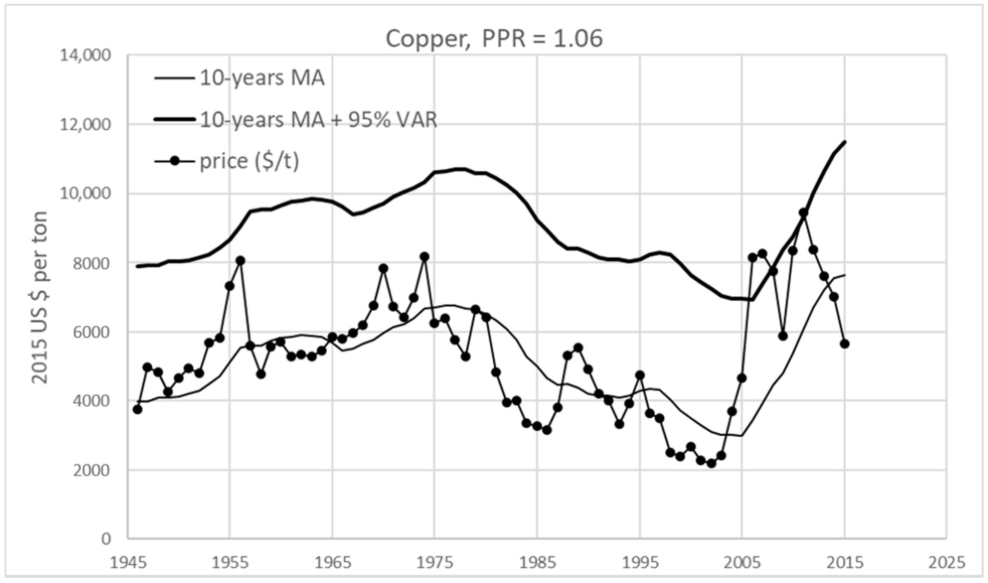
3.1. The PPR and Price Charts of 42 Raw Materials

The values of 95% VAR and the PPR were determined for 42 metals, based on USGS data [47], which provide yearly prices of metals as of 1900 for common metals. For less common metals, most prices are known since the Second World War.

Figure 4, Figure 5, Figure 6 and Figure 7 show the prices, the 10-year MA, and the 10-year MA + eco-costs as a function of time. The two examples of copper and cobalt show that these materials have quite high price peaks (PPR of approximately 1) leading to a high business risk in terms of the costs of material supply. Magnesium and aluminum have a low business risk. The graphs of the other metals can be found in the Supplementary Materials [46]. Note that the price range of the USGS [47] was extended with estimates for cobalt and lithium by the authors, to enable the calculations on car batteries for the business case in Appendix A.

A list of VAR and PPR scores for all 42 metals is provided in

Table 2. The price peak ratio (PPR) and the value at risk (VAR) 95th percentile (eco-costs) of 42 metals.

Metal	PPR	VAR (95)	Metal	PPR	VAR (95)
		$/kg			$/kg
Aluminum, Al	0.32	0.95	Manganese, Mn	0.56	0.48
Antimony, Sb	1.29	8.45	Mercury, Hg	1.18	37.69
Arsenic, As	0.66	1.01	Molybdenum, Mo	2.12	48.18
Barium, Ba	0.47	0.039	Nickel, Ni	1.01	12.58
Beryllium, Be	0.18	249	Niobium, Nb	1.43	37.46
Bismuth, Bi	1.02	23.64	Platinum, Pt	0.53	8660
Boron, B	0.28	0.36	Rhenium, Re	2.87	5340
Cadmium, Cd	0.93	18.1	Selenium, Se	2.64	94.62
Cesium, Cs	no data	no data	Silicon, Si	0.48	1.1
Chromium, Cr	0.75	1.01	Silver, Ag	1.29	605
Cobalt, Co	1.1	45.16	Strontium, Sr	0.84	0.38
Copper, Cu	1.06	3.94	Tantalum, Ta	4.24	627
Gallium, Ga	0.17	123	Tellurium, Te	1.14	108
Germanium, Ge	0.58	927	Thallium, Tl	1.21	3060
Gold, Au	1.14	25,290	Thorium, Th	0.86	119
Hafnium, Hf	0.91	253	Tin, Sn	0.78	19.06
Indium, In	1.14	667	Titanium, Ti	1.47	14.13
Iron (ore), Fe	0.86	0.046	Tungsten, W	0.78	32.26
Lead, Pb	0.82	1.52	Vanadium, V	0.94	22.16
Lithium, Li	0.6	2.97	Zinc, Zn	0.83	1.51
Magnesium, Mg	0.18	0.12	Zirconium, Zr	1.04	0.62

. In

Table A2. Resource scarcity indicators for metals.

Metal	CRM?	CRM Supply Risk *	Risk List Index **	Long-Term Scarcity ***
	(Yes/No)	(Range 0–10)	(Range 3.3–10)	(Year of Depletion)
Aluminum, Al	No	0.5	4.8	Over 3000
Antimony, Sb	Yes	4.3	9.0	2040
Arsenic, As	No	-	7.9	2490
Barium, Ba	Yes	1.6	7.6	Over 3000
Beryllium, Be	Yes	2.4	7.1	Over 3000
Bismuth, Bi	Yes	3.8	8.8	2190
Boron, B	No	-	-	2250
Cadmium, Cd	No	-	7.1	2590
Cesium, Cs	No	-	-	-
Chromium, Cr	No	0.9	6.2	2200
Cobalt, Co	Yes	1.6	8.1	Over 3000
Copper, Cu	No	0.2	4.8	2170
Gallium, Ga	Yes	1.4	8.6	Over 3000
Germanium, Ge	Yes	1.9	8.6	Over 3000
Gold, Au	No	0.2	4.5	2055
Hafnium, Hf	Yes	1.3	-	-
Indium, In	No	2.4	8.1	Over 3000
Iron (ore), Fe	No	0.8	5.2	2380
Lead, Pb	No	0.1	5.5	2300
Lithium, Li	No	1.0	7.6	Over 3000
Magnesium, Mg	Yes	4.0	7.6	Over 3000
Manganese, Mn	No	0.9	5.7	Over 3000
Mercury, Hg	No	-	6.9	Over 3000
Molybdenum, Mo	No	0.9	8.1	2100
Nickel, Ni	No	0.3	5.7	2370
Niobium, Nb	Yes	3.1	6.7	Over 3000
Platinum, Pt	Yes	2.1	7.6	Over 3000
Palladium, Pd	Yes	1.7	7.6	Over 3000
Iridium, Ir	Yes	2.8	7.6	Over 3000
Osmium, Os	Yes	-	7.6	Over 3000
Rhodium, Rh	Yes	2.5	7.6	Over 3000
Ruthenium, Ru	Yes	3.4	7.6	Over 3000
Rhenium, Re	No	1.0	7.1	2130
Selenium, Se	No	0.4	6.9	Over 3000
Silicon, Si	Yes	1.0	-	-
Silver, Ag	No	0.5	7.1	2290
Strontium, Sr	No	-	8.3	Over 3000
Tantalum, Ta	Yes	1.0	7.1	Over 3000
Tellurium, Te	No	0.7	-	-
Thallium, Tl	No	-	-	Over 3000
Thorium, Th	No	-	5.7	-
Tin, Sn	No	0.8	6.0	2280
Titanium, Ti	No	0.3	4.8	Over 3000
Tungsten, W	Yes	1.8	8.1	Over 3000
Vanadium, V	Yes	1.6	8.6	Over 3000
Zinc, Zn	No	0.3	4.8	2100
Zirconium, Zr	no	-	6.4	Over 3000

* European Commission (2017) [3]; ** British Geological Survey (2015) [1]; *** Henckens (2016) [13].

(Appendix B), the scores are summarized of the CRM system of the European Commission [3], the risk list scores of the British Geological Survey [1], and the expected year of absolute depletion, as estimated by Henckens [13].

Calculations of the 95% VAR of rare-earth element (REE) metals cannot be made at this time, because of the lack of historical data. Estimates on the eco-costs are given in the Supplementary Materials [46], applying a simplified method to calculate the PPR.

There is a remarkable issue in all these figures; they hardly correlate with each other, and they do not correlate with the oil prices either (even the price of aluminum, for which production is rather energy intensive, does not correlate with the oil price). This phenomenon underlines the fact that each supply chain of each individual metal is unique (which confirms the conclusion of Reference [36] in Section 1.2).

3.2. The Potential Application of the PPR and the VAR in LCA

In LCA, the PPR could be regarded as a kind of “midpoint” characterization factor for short-term scarcity of a metal. It should be multiplied by the price of that material to reach the level of an “endpoint” indicator. Equation (3) describes the financial tisk of a product with a material mass m.

FR = PPR × 10-year MA × m = 95% VAR × m,

(3)

where:

• FR = the Financial Risk of the scarcity of a metal in a product (US$, euro or any other currency),
• PPR = the Peak Price Ratio (dimensionless),
• 10-year MA = the average price for 10 years of a specific material in (US$/kg, euro/kg, or any other currency per kg),
• 95% VAR = the Value at Risk 95% (euro/kg, US$/kg, or any other currency) = eco-costs of materials scarcity,
• m = the mass of a specific material in the product (kg).

Equation (3) shows that the 95% VAR can be considered as a monetary endpoint characterization factor. It might be regarded as a prevention-based indicator, since the prevention measure is to add the required financial buffer, such that the sudden price jump only erodes the profit margin of the product, but not to a level of bankruptcy. The VAR is not a damage-based indicator, since the consequential damage might be much more (e.g., lay-offs caused by bankruptcy; see Figure 2).

The system of the eco-costs is a monetary single-indicator system in LCA [24,40,48], based on the sum of the (marginal) prevention costs (or abatement costs) of the midpoints, as depicted in Figure 8. It is widely applied in design and engineering, since it is related to the so-called “hidden” or “external” costs of a product or service. Recently, the long-term fixed-stock paradigm for scarcity (in the eco-costs 2007 and the eco-costs 2012) was abandoned, and replaced by the short-term supply risk approach (the eco-costs 2017), where the 95% VAR is equal to eco-costs of metals scarcity (euro/kg) (see Figure 8). The advantage of the eco-cost system is that it can combine environmental midpoints and social midpoints (human right violations, like child labor) into one single endpoint indicator, since the dimensions of all midpoints are the same (euro/kg). That enables LCA benchmarking of metals (mining plus refining) in a relative simple way, which is important for engineering, business strategies, and governmental policies.

4. Discussion

4.1. The Issue of By-Products in Mining

An important issue is the different situation for “carrier (host) metals” and “companion metals” [9]. Companion metals are mined as by-products from parent ores. The production of host metals is generally regarded as relatively flexible, which means that it can adapt to the market demand. For the by-products, however, the situation is less flexible by definition, since production quantities are linked to the production quantities of the host metals, leading to inelastic price characteristics.

An example of a by-product with oversupply is cadmium since 2000; a disruption will just lead to less oversupply; thus, high prices are not to be expected. An opposite example is cesium, which was in oversupply before 1990.

Such companion metals might have a sudden change in supply characteristics from structural oversupply to structural undersupply in the market, resulting in structural price shocks (other than the normal price peaks caused by temporary political unrest). Sprecher et al. [14] studied several such structural market demand changes, e.g., copper when it is replaced by graphene. It is obvious that the 95% VAR cannot predict these kinds of structural market changes and can, therefore, only be applied for a restricted time period (e.g., 30 years maximum). Another consequence of these kinds of structural changes in the supply chain is that the calculations on the VAR should be checked after every new release of USGS data.

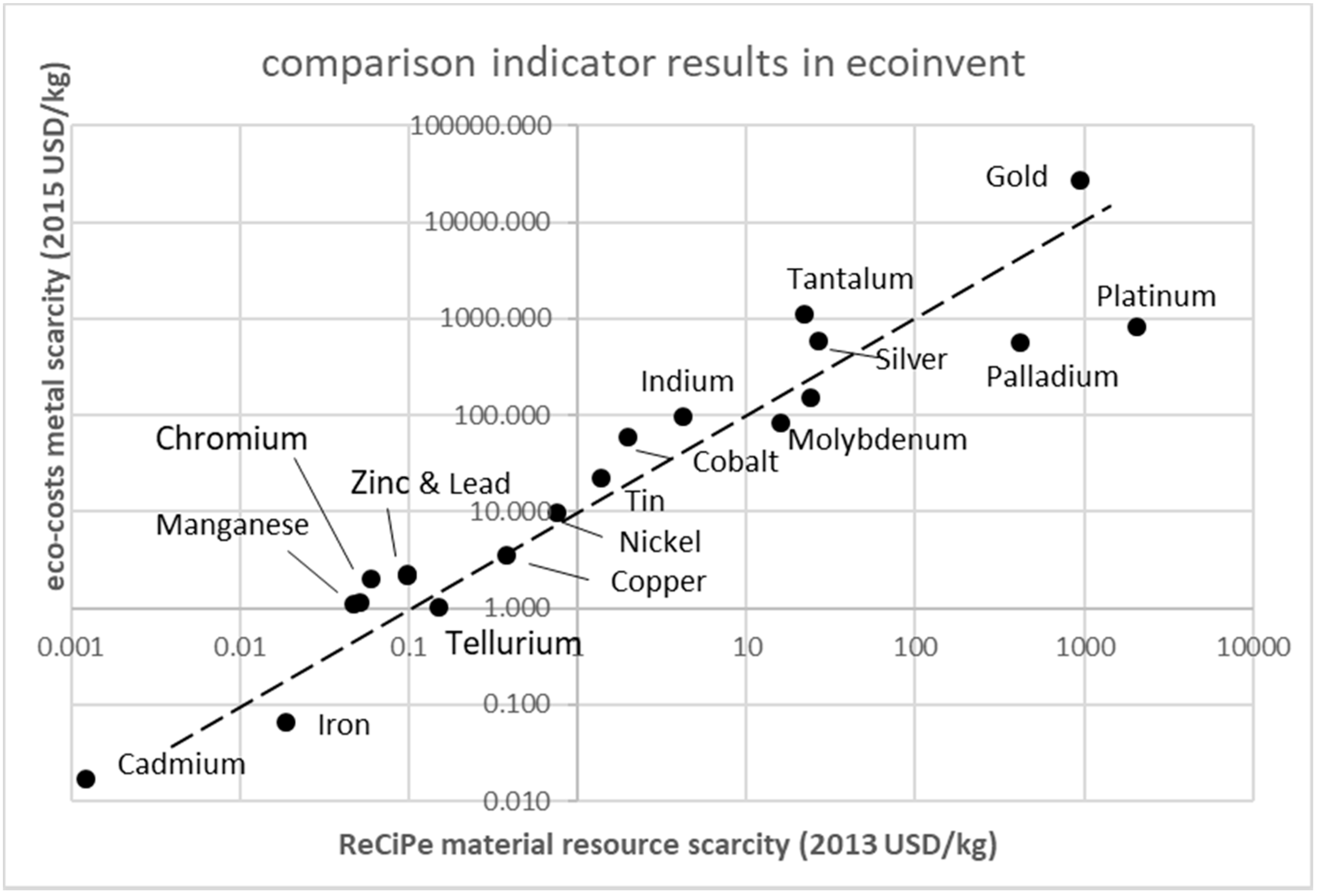
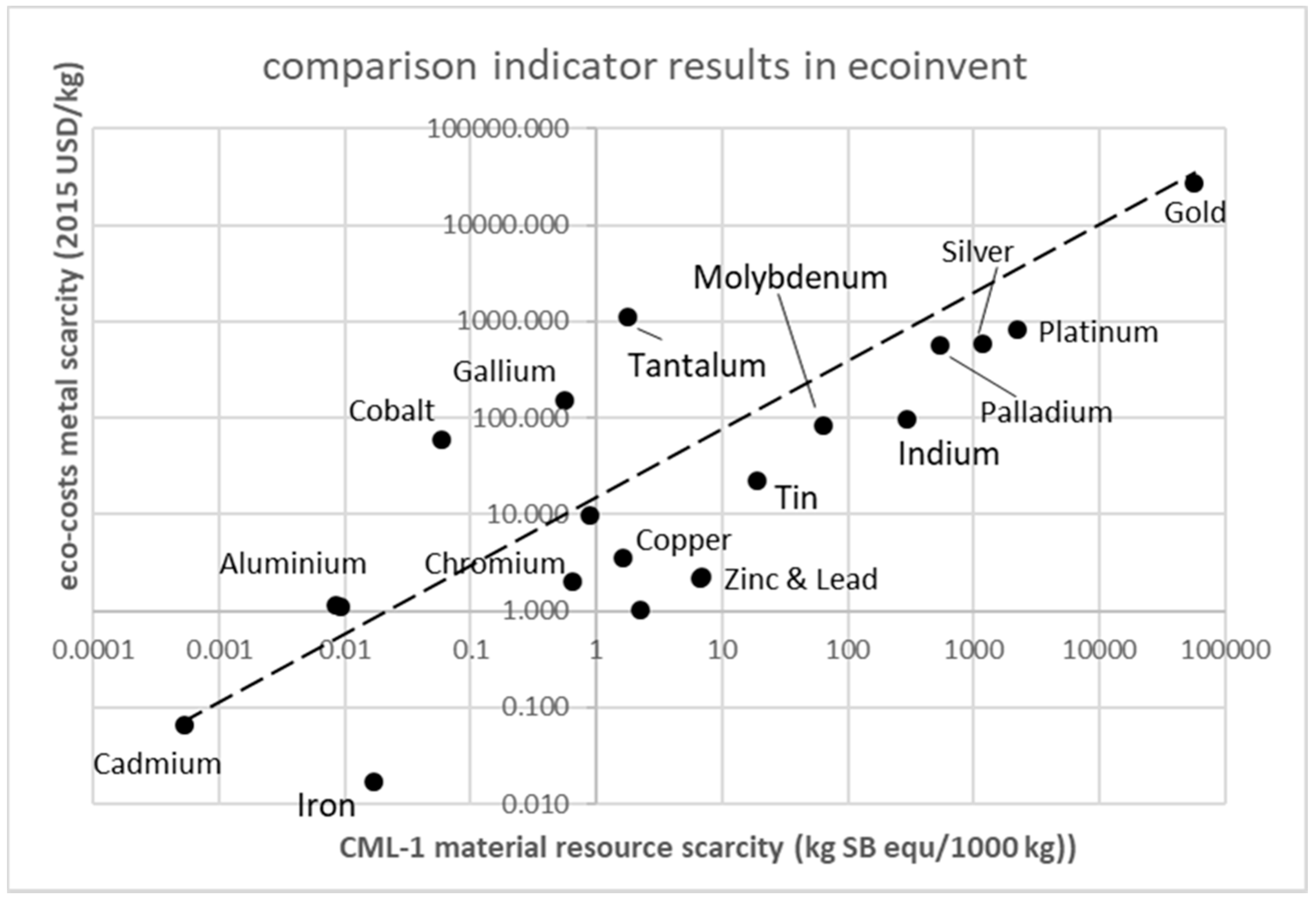
4.2. Validation Checks on the System Metrics

It was decided to base the analyses of this paper on the combination of the 95% VAR and the 10-year MA. The 95% VAR was chosen because it is a common practice in the financial world. The consequence of the 95% in the VAR calculation is that the large price jumps might occur every 20 years on average. The 10-year MA was selected after some experiments in the range of 5–10 years. For five, six, and seven years, the prediction was slightly worse than for eight, nine, and 10 years (there were no significant differences between eight and 10 years); thus, the calculation system is not very sensitive to the choice of the number of years, as long as it is not less than five. More than 10 years became unpractical and did not give improved results.

The disadvantage of applying the 95% VAR for the eco-costs of metal scarcity is that it does not describe how much higher the price jump is compared to the 95% VAR + 10-year MA (see Figure 3). Analyzing the price jumps of all 42 metals (see also the price charts in the Supplementary Materials [46]) reveals that, for 32 metals, this is not an important issue, since all prices remained below or near the MA + VAR limit. Single price jumps of 14 metals, however, were higher than a level of +50% additional to the VAR: barium (barite), 69% in 2012; chromium, 147% in 2008; cobalt, 211% in 1979; gold, 62% in 1980; lithium, 169% in 2018; manganese, 262% in 2008; mercury, 81% in 1965; molybdenum, 198% in 1979; nickel, 149% in 2007; silver, 134% in 1980; tellurium, 145% in 2011; vanadium, 181% in 2005; zinc, 68% in 2006; and zirconium, 239% in 2011.

Another issue is the question of how well an indicator from the past predicts the future. Since we do not know the future, the only way to make a validation check on this issue is to “step back in the past”, to year B, calculate the eco-costs (=VAR) for the row of years 1946–year B, and check then how well the prices after year B stay under the eco-costs + 10-year MA.

Such a validation check was done by simulating a business case that resembles the business case of Appendix A. Suppose that a trader guarantees a fixed sale price at year B for the next five or 10 years at a level of the 10-year MA plus the eco-costs of that year B. At constant market prices, this is a good deal, since the trader can buy the metal at the market price and sell it for an extra price (the eco-costs). The question is then how much capital this trader might lose in in years with price peaks, since he/she might have to buy that metal in some years at peak prices higher than the MA + eco-costs of year B. Figure 4, Figure 5, Figure 6 and Figure 7 show that there is no problem for aluminum, magnesium, and cobalt, but price peaks of copper after 2005 will cause years of losses for the trader (note that the VAR of 1946–2005 will be lower than the VAR of 1946–2015). Simulations were done for periods of five years and 10 years, starting at year B = 1995, and starting at year B = 2005. The results of these simulations for 32 common metals (the metals for which a full dataset 1946–2015 is available) are provided in the Excel file of the Supplementary Materials [46]. These simulations were done for aluminum, antimony, arsenic, barite, beryllium, bismuth, boron, cadmium, chromium, cobalt, copper, iron, gold, indium, lead, lithium, manganese, mercury, magnesium, molybdenum, nickel, platinum, selenium, silver, silicon, strontium, tellurium, tin, tungsten, vanadium, zinc, and zirconium.

Table 3. The “average losses by price peaks”/eco-costs: the results of a simulation in the case of the trader for 32 metals in total.

Calculation Period of VAR	Period of Simulation	“Average Losses by Price Peaks”/Eco-Costs (%)
VAR calculated for 1946–2015	1996–2000	0.00%
	1996–2005	0.76%
	2006–2010	7.83%
	2006–2015	10.32%
VAR calculated for 1946–1995	1996–2000	0.00%
	1996–2005	1.44%
VAR calculated for 1946–2005	2006–2010	22.43%
	2006–2015	30.14%

gives the summary of these simulation results.

These results show the sensitivity to the choice of the VAR; when the VAR does not include the relative volatile period of 2005–2015 (i.e., the data of the VAR calculated for 1946–2005), the calculation shows relatively greater “average losses by price peaks” in this period. As such, this is logical, but it shows the imperfection of the VAR as an absolute predictor of prices. Further research is needed here to improve the prediction capabilities of the calculation system, coping with multi-year “pig cycles”. Note that, for the 32 metals of this simulation run, the eco-costs are equal to the “VAR calculated for 1946–2015”.

4.3. Validation in LCA

In LCA, an LCA practitioner might be misled by the results of LCA calculations on resource indicators. The issue here is that most LCI databases provide cradle-to-gate data, often including the required infrastructure (for mining and the required energy), and apply their own allocation methods. A metal that has a tiny fraction in the life-cycle inventory list, however, with a high depletion score, might govern the LCA calculation of the metal that is under study. As an example, the ADP scores per kg of metal were calculated on the basis of Ecoinvent data (see

Table A3. The main component in the calculation of the ADP, ReCiPe, and eco-costs, based on life-cycle inventory (LCI) lists of Ecoinvent version 3.4.

	in ADP		in ReCiPe Metal Depletion		in Eco-costs (95% VAR)
	Dominated by (%)		Dominated by (%)		Dominated by (%)
Aluminum	Cadmium	34%	Aluminum	97%	Aluminum	99%
Cadmium	Cadmium	29%	Nickel	27%	Nickel	36%
Chromium	Chromium	97%	Chromium	52%	Chromium	70%
Cobalt	Cobalt	35%	Cobalt	100%	Cobalt	100%
Copper	Copper	72%	Copper	53%	Copper	97%
Gallium	Cadmium	16%	Gallium	100%	Gallium	99%
Gold	Gold	100%	Gold	99%	Gold	100%
Indium	Cadmium	51%	Lead	43%	Zinc	45%
Lead	Cadmium	51%	Lead	43%	Zinc	45%
Manganese	Manganese	69%	Manganese	87%	Manganese	97%
Molybdenum	Copper	62%	Molybdenum	56%	Molybdenum	51%
Nickel	Copper	81%	Nickel	68%	Nickel	80%
Palladium	Copper	48%	Platinum	48%	Palladium	61%
iron	Cadmium	22%	Iron	100%	Iron	98%
Platinum	Platinum	70%	Platinum	70%	Palladium	49%
Silver	Silver	46%	Silver	60%	Silver	47%
Tantalum	Copper	35%	Tantalum	99%	Tantalum	100%
Tellurium	Copper	23%	Copper	57%	Copper	71%
Tin	Tin	100%	Tin	100%	Tin	100%
Zinc	Cadmium	50%	Lead	42%	Zinc	45%

Example 1: the main component of the total ADP of 1 kg of aluminum is the APD of the cadmium in the LCI (34% of the total score). Example 2: the main component of the total ReCiPe metal depletion of 1 kg of aluminum is the score of aluminum itself the LCI (97% of the total score).

in Appendix C). This table shows, for instance, that the ADP of 1 kg of nickel is 80% determined by the copper in the LCI. As such, this is alright from a theoretical point of view, under the assumption that the infrastructural data are very accurate. Given the fact that, in practice, most LCIs do not have very accurate infrastructural data (i.e., the real supply chain differs from the generalized assumptions), the issue becomes realistic whether or not the right metals are selected by such an LCA, regardless of the correctness of a philosophy behind such a calculation system. Drielsema [16] questions the validity of LCA decisions from a philosophical and practical point of view (each philosophy has its own score system and, hence, its own preferences), highlighting the problem of the wide range of indicator scores in ADP as a mathematical and/or methodical issue.

The wide range of scores in the ADP system is a consequence of R² in Equation (2). This R² results in a data range of more than 1.0 × 10¹⁰ in the “CML-1 baseline system, Version 3”. It goes from 52 (gold) to 2.02 × 10⁻⁹ (magnesium), 1.09 × 10⁻⁹ (aluminum), and 1.40 × 10⁻¹¹ (Silicon). Similarly, the data range of the “CML-1A non baseline system, Version 3” goes from 1.95 × 10⁴ (germanium) to 1.66 × 10⁻⁶ (iron). Note the large difference between CML-1 baseline and CML-1A non-baseline.

The indicator of the mineral resource scarcity of ReCiPe has a more satisfactory result in LCA calculations, since it has a less wide range of 1.9 × 10⁵: from 2.73 × 10³ $/t (cesium) to 1.43 × 10⁻² $/t (iron). The eco-cost (95% VAR) has a similar range of 1 × 10⁶ (from 50,000 $/t for cesium to 0.046 $/t for iron). ReCiPe and eco-costs have a better performance in LCA as far as the “what you see is what you get” issue (see Table A3).

The issue of Drielsema et al. [16], with regard to the validity of decisions in LCA (i.e., does the lowest score relate to the material with the lowest scarcity in reality?), can never be resolved, given all the uncertainties. However, Figure 9 shows an interesting comparison between the eco-costs, based on the 95% VAR, and the material resource scarcity indicator in ReCiPe, based on the fixed-stock paradigm. Although both philosophies are completely different, the ranking of metals seems only slightly influenced by the choice of the indicator system. This is not the case for the CML-1 indicator, which results in another sequence of preferences as far as a metal scarcity is concerned (see Figure 10).

5. Conclusions

In this paper, an indicator system was developed for the issue of scarcity. With regard to research question 1 (“Which statistical method can be regarded as suitable to predict the future risk of a sudden jump in prices caused by disruptions in the supply chain?”), it was concluded that the value at risk (VAR) seems to be a suitable way to describe the scarcity of metals for the short term (10–30 years). The 95% criterion is a reasonable compromise between a relevant risk level (i.e., on average, one price jump per period of 20 years) and the available dataset (the past 70 years).

With regard to research question 2 (“For which metals are these price fluctuations relevant, i.e., are the price peaks high in comparison to the average price over a decade?”), it was concluded that the following 15 out of 42 metals have the risk of a sudden price jump which is equal to or more than the average price of the previous 10 years (i.e., PPR is higher than 1; see Table 2): antimony, bismuth, cobalt, gold, indium, mercury, molybdenum, niobium, rhenium, selenium, tantalum, tellurium, thallium, tungsten, and zirconium. In general, there is no correlation with the long-term depletion, nor with the risk list index and the CRM supply risk (see Appendix B, Table A2).

With regard to research question 3 (“How can this approach of supply chain risks and consequential price jumps be incorporated in LCA?”), it was concluded that the 95% VAR can be directly applied as a prevention-based endpoint indicator in LCA (e.g., the system of eco-costs), since the direct negative impact of the price jump can be mitigated by a monetary buffer of the same size (the pathway of Figure 2 is then stopped under the block “deteriorating profit margins”).

It can be concluded that the eco-cost of material scarcity is a more meaningful indicator than the long-term scarcity indicators that are based on the fixed-stock paradigm. The peak price ratio (PPR) can be regarded as a practical indicator for socio-economical risks of the supply of metals for the short term (10–30 years). It is suitable for business product innovation strategies, as well as governmental policies, and moves beyond current critical material thinking.

The sequence of the scarcity indicators for metals in LCA (from a low score to a high score) is similar in both the eco-cost system and the ReCiPe system; however, in ADP, the sequence is quite different. Although, in theory, it is acceptable to apply the VAR and the ADP next to each other, since these midpoints have different “areas of projection” (i.e., the future generations versus the current generation), it is recommended to avoid the use of ADP, since the high inaccuracy of this indicator might give misleading results. A combination with the mineral resource scarcity indicator of ReCiPE does make more sense.

Further research is needed to find a solution for the problem of the companion metals (co-production) that switch from structural overproduction (ultra-low prices) to structural overdemand (high price peaks) and vice versa, since the proposed system in this paper cannot properly cope with such a structural change of the supply chain characteristics. In the database of 42 metals, this was the case for two metals in the last 70 years: cobalt and cesium. This research might go hand-in-hand with a more sophisticated statistical approach for the other 40 materials (e.g., including multi-year seasonality).

References

1. British Geological Survey Risk List. 2015. Available online: https://www.bgs.ac.uk/mineralsuk/statistics/riskList.html (accessed on 21 October 2018).
2. Schulz, K.J.; DeYoung, J.H., Jr.; Bradley, D.C.; Seal, R.R., II. Critical Mineral Resources of the United States—An Introduction; United States Geological Survey: Reston, VA, USA, 2017. [CrossRef]
3. European Commission. Study on the Review of the List of Critical Raw Materials. 2017. Available online: https://publications.europa.eu/en/publication-detail/-/publication/08fdab5f-9766-11e7-b92d-01aa75ed71a1/language-en (accessed on 12 October 2018).
4. Schmidt, M. Scarcity and Environmental Impact of Mineral Resources—An Old and Never-Ending Discussion. Resources 2019, 8, 2. [Google Scholar] [CrossRef]
5. Guinée, J.; Heijungs, R. A proposal for the definition of resource equivalency factors for use in product life-cycle assessment. Environ. Toxicol. Chem. 1995, 14, 917–925. [Google Scholar] [CrossRef] [Green Version]
6. Van Oers, L.; de Koning, A.; Guinée, J.B.; Huppes, G. Abiotic Resource Depletion in LCA: Improving Characterisation Factors for Abiotic Resource Depletion as Recommended in the New Dutch LCA Handbook; Road and Hydraulic Engineering Institute, Ministry of Transport and Water: Amsterdam, The Netherlands, 2002.
7. Van Oers, L.; Guinee, J. The Abiotic Depletion Potential: Background, Updates, and Future. Resources 2016, 5, 16. [Google Scholar] [CrossRef]
8. Schneider, L.; Berger, M.; Finkbeiner, M. Abiotic resource depletion in LCA—Background and update of the anthropogenic stock extended abiotic depletion potential (AADP) model. Int. J. Life Cycle Assess. 2015, 20, 709–721. [Google Scholar] [CrossRef]
9. Graedel, T.E.; Barr, R.; Cordier, D.; Enriquez, M.; Hagelüken, C.; Hammond, N.Q.; Kesler, S.; Mudd, G.; Nassar, N.; Peacey, J.; et al. Estimating Long-Run Geological Stocks of Metals; UNEP International Panel on Sustainable Resource Management; Working Group on Geological Stocks of Metals; Working Paper, 11 June 2011; UNEP: Nairobi, Kenya, 2011. [Google Scholar]
10. Wilkinson, B.H.; Kesler, S.E. Strüngman forum reports. In Linkages of Sustainability; Graedel, T.E., van der Voet, E., Eds.; The MIT Press: Cambridge, MA, USA, 2010; p. 122. [Google Scholar]
11. Speirs, J.; McGlade, C.; Slade, R. Uncertainty in the availability of natural resources: Fossil fuels, critical metals and biomass. Energy Policy 2015, 87, 654–664. [Google Scholar] [CrossRef] [Green Version]
12. Mudd, G.M.; Yellishetty, M.; Reck, B.K.; Graedel, T.E. Quantifying the Recoverable Resources of Companion Metals: A Preliminary Study of Australian Mineral Resources. Resources 2014, 3, 657–671. [Google Scholar] [CrossRef]
13. Henckens, M.L.C.M. Managing Raw Materials Scarcity: Safeguarding the Availability of Geologically Scarce Mineral Resources for Future Generations. Ph.D. Thesis, University of Utrecht, Utrecht, The Netherlands, 2016. [Google Scholar]
14. Sprecher, B.; Reemeyer, L.; Alonso, E.; Kuipers, K.; Graedel, T.E. How “black swan” disruptions impact minor metals. Resources Policy 2017, 54, 88–96. [Google Scholar] [CrossRef]
15. Singer, D.A. Future copper resources. Ore Geol. Rev. 2017, 86, 271–279. [Google Scholar] [CrossRef]
16. Drielsma, J.A.; Russell-Vaccari, A.J.; Drnek, T.; Tom Brady, T.; Weihed, P.; Mistry, M.; Perez Simbor, L. Mineral resources in life cycle impact assessment—Defining the path forward. Int. J. Life Cycle Assess. 2016, 21, 85–105. [Google Scholar] [CrossRef]
17. Chapman, F.P.; Roberts, F. Metal Resources and Energy; Butterworth Scientific: Oxford, UK, 1983. [Google Scholar]
18. Dewulf, J.; Van Langenhove, H.; Muys, B.; Bruers, S.; Bakshi, B.R.; Grubb, G.F.; Paulus, D.M.; Sciubba, E. Exergy: Its potential and limitations in environmental science and technology. Environ. Sci. Technol. 2008, 42, 2221–2232. [Google Scholar] [CrossRef]
19. Liao, W.; Heijungs, R.; Huppes, G. Thermodynamic resource indicators in LCA: A case study on the Titania produced in Panzhihua city, southwest China. Int. J. Life Cycle Assess. 2012, 17, 951–961. [Google Scholar] [CrossRef]
20. Goedkoop, M.; Spriensma, R. The Eco-Indicator 99, a Damage Oriented Method for Life Cycle Impact Assessment; Pre Consultants BV: Amersfoort, The Netherlands, 2001. [Google Scholar]
21. Goedkoop, M.; Heijungs, R.; Huijbregts, M.A.J.; De Schryver, A.; Struijs, J.; Van Zelm, R. Mineral Resource Depletion in ReCiPe 2008: A life cycle impact assessment method which comprises harmonised category indicators at the midpoint and the endpoint level. In Report I: Characterisation Factors, 1st ed.; Ministerie van Volkhuisvesting, Ruimtelijke Ordening en Milieubeheer: Den Haag, The Netherlands, 2008. [Google Scholar]
22. Vieira, M.D.M.; Ponsioen, T.C.; Goedkoop, M.J.; Huijbregts, M.A.J. Surplus Cost Potential as a Life Cycle Impact Indicator for Metal Extraction. Resources 2016, 5, 2. [Google Scholar] [CrossRef]
23. Rötzer, N.; Schmidt, M. Decreasing Metal Ore Grades—Is the Fear of Resource Depletion Justified? Resources 2018, 7, 88. [Google Scholar] [CrossRef]
24. Vogtländer, J.G.; Brezet, H.C.; Hendriks, C.F. The virtual Eco-costs ‘99: A single LCA-based indicator for sustainability and the Eco-costs—Value ratio (EVR) model for economic allocation: A new LCA-based calculation model to determine the sustainability of products and services. Int. J. Life Cycle Assess. 2001, 6, 157–166. [Google Scholar] [CrossRef]
25. Hotelling, H. The economics of Exhaustible Resources. J. Political Econ. 1931, 39, 137–175. [Google Scholar] [CrossRef]
26. Frischknecht, R.; Büsser Knöpfel, S. Ecological scarcity 2013—New features and its application in industry and administration—54th LCA forum, Ittigen/Berne, Switzerland, December 5, 2013. Int. J. Life Cycle Assess. 2014, 19, 1361–1366. [Google Scholar] [CrossRef]
27. Steen, B. Calculation of Monetary Values of Environmental Impacts from Emissions and Resource Use. J. Sustain. Dev. 2016, 9. [Google Scholar] [CrossRef]
28. Laurent, A.; Olsen, S.I.; Hauschild, M.Z. Normalization in EDIP97 and EDIP2003: Updated European inventory for 2004 and guidance towards a consistent use in practice. Supplementary Material. Int. J. Life Cycle Assess. 2011, 16, 401–409. [Google Scholar] [CrossRef]
29. EN 15804: 2012+ A1: 2013: Sustainability of Construction Works. Environmental Product Declarations. Core Rules for the Product Category of Construction Products. Available online: https://shop.bsigroup.com/ProductDetail/?pid=000000000030279721 (accessed on 18 April 2019).
30. European Commission, Joint Research Centre, Institute for Environment and Sustainability. Characterisation Factors of the ILCD Recommended Life Cycle Impact Assessment Methods. Database and Supporting Information, 1st ed.; EUR 25167; Publications Office of the European Union: Luxembourg, 2012. [Google Scholar]
31. Jolliet, O.; Margni, M.; Charles, R.; Humbert, S.; Payet, J.; Rebitzer, G.; Rosenbaum, R. IMPACT 2002+: A new life cycle impact assessment methodology. Int. J. Life Cycle Assess. 2003, 8, 324. [Google Scholar] [CrossRef]
32. Graedel, T.E.; Reck, B.K. Six Years of Criticality Assessments, What have we learned so far? Forum Yale Univ. 2015, 20. [Google Scholar] [CrossRef]
33. Schneider, L.; Berger, M.; Schüler-Hainsch, E.; Knöfel, S.; Ruhland, K.; Mosig, J.; Bach, V.; Finkbeiner, M. The economic resource scarcity potential (ESP) for evaluating resource use based on life cycle assessment. Int. J. Life Cycle Assess. 2014, 19, 601–610. [Google Scholar] [CrossRef]
34. Dewulf, J.; Benini, L.; Mancini, L.; Sala, S.; Andrea Blengini, G.; Ardente, F.; Recchioni, M.; Maes, J.; Pant, R.; Pennington, D. Rethinking the Area of Protection “Natural Resources” in Life Cycle Assessment. Environ. Sci. Technol. 2015, 49, 5310–5317. [Google Scholar] [CrossRef]
35. Sonnemann, G.; Gemechu, E.D.; Adibi, N.; De Bruille, V.; Bulle, C. From a critical review to a conceptual framework for integrating the criticality of resources into Life Cycle Sustainability Assessment. J. Clean. Prod. 2015, 94, 20–34. [Google Scholar] [CrossRef]
36. Achzet, B.; Helbig, C. How to evaluate raw material supply risk—An overview. Resour. Policy 2013, 38, 435–447. [Google Scholar] [CrossRef]
37. European Commission. Methodology for Establishing the EU List of Critical Raw Materials—Guidelines; European Commission: Luxembourg, 2017; ISBN 978-92-79-68051-9. [Google Scholar]
38. UNEP. Recycling Rates of Metals. A Status Report of the International Resource Panel. 2011. Available online: http://www.unep.org/resourcepanel/Portals/24102/PDFs/Metals_Recycling_Rates_110412-1.pdf (accessed on 18 April 2019).
39. Mancini, L.; Benini, L.; Sala, S. Characterization of raw materials based on supply risk indicators for Europe. Int. J. Life Cycle Assess. 2018, 23, 726–738. [Google Scholar] [CrossRef]
40. Vogtlander, J. The model of the Eco-Costs/Value Ratio. Ph.D. Thesis, Delft University of Technology, Delft, The Netherlands, 2001. [Google Scholar]
41. Peck, D.; Kandachar, P.; Tempelman, E. Critical materials from a product design perspective. Mater. Des. 2015, 65, 147–159. [Google Scholar] [CrossRef]
42. Peck, D. Prometheus Missing: Critical Materials and Product Design; Delft University of Technology: Delft, The Netherlands, 2016; ISBN 9-789065-63997. [Google Scholar] [CrossRef]
43. Tapia Cortez, C.A.; Saydam, S.; Coulton, J.; Sammut, C. Alternative techniques for forecasting mineral commodity prices. Int. J. Min. Sci. Technol. 2018, 28, 309–322. [Google Scholar] [CrossRef]
44. Taleb, N.N. Fooled by Randomness; Texere: London, UK, 2001; ISBN 1-58799-071-7. [Google Scholar]
45. Taleb, N.N. The Black Swan: The Impact of the Highly Improbable; Penguin: London, UK, 2007; ISBN 978-0-14103459-1. [Google Scholar]
46. Supplementary Materials. Available online: www.ecocostsvalue.com/EVR/scarcity.html (accessed on 15 March 2019).
47. Kelly, T.D.; Matos, G.R. Historical Statistics for Mineral and Material Commodities in the United States, USGS 2015. Available online: https://minerals.usgs.gov/minerals/pubs/historical-statistics/ (accessed on 21 October 2018).
48. Van der Velden, N.M.; Vogtlander, J.G. Monetisation of external socio-economic costs of industrial production: A social-LCA-based case of clothing production. J. Clean. Prod. 2017, 153, 320–330. [Google Scholar] [CrossRef]
49. Vogtlander, J. A Practical Guide to LCA for Students, Designers and Business Managers, 5th ed.; Delft Academic Press: Delft, The Netherlands, 2017; ISBN 97890-6562-3614. Available online: https://en.wikipedia.org/wiki/Eco-costs (accessed on 15 March 2019).
Figure 1. The price history per ton of copper since 1900 in United States dollars (US$) 2015. Average decline per year: 0.3%. Henckens [13] recalculated.
Sustainability 11 02446 g001
Figure 2. The cause–effect pathway of the socio-economic effects of resource scarcity.
Sustainability 11 02446 g002
Figure 3. The PPR (price peak ratio) explained as a function of the 95% value at risk (VAR) and the 10-year moving average (MA). Note: The 10-year MA line goes gradually up and down during the decennia, following periods of price peaks and economic “pig cycles” (example of lead prices around 1975).
Sustainability 11 02446 g003
Figure 4. The price of copper in 2015 US$ per ton, the 10-year MA, and the MA + eco-costs, where the eco-costs = 95% VAR. Years with extreme price jumps are 2006, 2007, and 2011.
Sustainability 11 02446 g004
Figure 5. The price of cobalt in 2015 US$ per ton, the 10-year MA, and the MA + eco-costs, where the eco-costs = 95% VAR. Years with extreme price jumps are 1979, 1980, and 1995.
Sustainability 11 02446 g005
Figure 6. The price of magnesium in 2015 US$ per ton, the 10-year MA, and the MA + eco-costs, where the eco-costs = 95% VAR. Years with extreme price jumps are 1957, 1985, and 2004.
Sustainability 11 02446 g006
Figure 7. The price of aluminum in 2015 US$ per ton, the 10-year MA, and the MA + eco-costs, where the eco-costs = 95% VAR. Years with extreme price jumps are 1979, 1988, and 2006.
Sustainability 11 02446 g007
Figure 8. The eco-costs of metal scarcity as part of the total eco-cost system in life-cycle assessment (LCA) [49].
Sustainability 11 02446 g008
Figure 9. A comparison between the metal scarcity indicators of the eco-cost system and ReCiPe, on the basis of calculation results in Ecoinvent V3.4. Note that the sequence for both indicator systems (from a low score to a high score) is almost the same, except for tellurium, molybdenum, tantalum, and gold.
Sustainability 11 02446 g009
Figure 10. A comparison between the metal scarcity indicator of the eco-cost system and the abiotic depletion potential (ADP) of CML-1, on the basis of calculation results in Ecoinvent V3.4. Note that the sequence for both indicator systems (from a low score to a high score) is not the same.
Sustainability 11 02446 g010