Article

Beyond the City: Effects of Urbanization on Rural Residential Energy Intensity and CO2 Emissions

1
Center for Agricultural Policy (CCAP), Peking University, Beijing 100871, China
2
School of Economics, Southwest University of Political Science and Law (SWUPL), Chongqing 401120, China
3
Biogas Institute of Ministry of Agriculture and Rural Affairs, Chinese Academy of Agricultural Science, Chengdu 610041, China
4
College of P.E. and Sports, Beijing Normal University, Beijing 100875, China
*
Author to whom correspondence should be addressed.
Sustainability 2019, 11(8), 2421; https://doi.org/10.3390/su11082421
Submission received: 21 March 2019 / Revised: 9 April 2019 / Accepted: 18 April 2019 / Published: 24 April 2019
(This article belongs to the Section Energy Sustainability)

Abstract

:
Trends of rural residential energy consumption and CO2 emission should be evaluated in a broader context of urbanization, especially in developing countries where urbanization is in its expanding stage. In this study, we use the STIRPAT model and various panel regression techniques to explore the impact of urbanization on rural residential energy consumption and CO2 emission by using data from Southwest China. The results show that a higher urbanization level contributes to higher total residential energy intensity. Increases in net income per capita can decrease the intensities of traditional biomass energy and non-biomass energy, while industrialization has a negative effect only on non-biomass energy intensity. Land use change driven by urbanization can also lower the intensities of total residential energy, traditional biomass energy and non-biomass energy. Moreover, the impact of total residential energy intensity on emissions is positive. Particularly, traditional biomass energy accounts for most of CO2 emissions derived from the use of residential energy. As urbanization is expected to increase in the developing world and lead to more CO2 emissions from rural areas, policies which intend to reduce the intensity of traditional biomass energy, promote biogas and industrialization, and raise net income of rural residents can be used as effective mitigation strategies.

1. Introduction

It is widely accepted that urbanization is a dynamic phenomenon of socioeconomic modernization that involves social, economic and ecological transformations in developing countries. Socially and economically, it refers to a process of concentrating population and economic activities in urban areas, while ecologically, it influences the functioning of local and global ecosystems by changing land use and land cover [1]. Through these processes, the world has undergone rapid urbanization in recent decades, with the share of the world urban population increasing from 34% in 1960 to 55% in 2017 [2]. Furthermore, the urban population is projected to be about 6.7 billion by 2050, accounting for 68% of the total world population [3]. To cope with the inevitable problems arising from such unprecedented growth, such as excessive consumption of resources, environmental pollution and ecosystem deterioration, the issue of how changes in urbanization affect energy consumption and its related CO2 emissions should be taken into careful consideration for designing sustainable development and climate change policies.
In recent years, although an increasing number of studies have investigated the relationship between urbanization and various environmental issues [4], the effects that urbanization has on energy use (intensity) and CO2 emissions are difficult to estimate. Due to urbanization, a substantial labor force shifts from primary agriculture to urban-based industries [4]. As a result, settlement patterns and production structures greatly change in rural areas, bringing dual effects to rural energy consumption and CO2 emissions [5,6]. The fast-paced urbanization gives rise to economies of scale and promotes technical innovation for increases in energy-using efficiency, lowering energy consumption and CO2 emissions [7,8]. Conversely, growing urbanization has led to a higher concentration of energy use (and higher intensity of energy use) that has adversely affected air quality and climate conditions (generating more CO2 emissions) through shifting production from less to more energy-intensive sources and increasing the number of vehicles and transport activities [9,10]. As little consensus has been reached on how urbanization exactly effects energy consumption and its related CO2 emissions, this provides the basic motivation for this paper to investigate the aggregate effects of urbanization on rural energy consumption and CO2 emissions. Nevertheless, this paper makes two major contributions to the existing literature. First, numerous researchers show that urbanization increases energy demand, leading to more CO2 emissions [7,8,11,12], but most of them have tended to only focus on the effects of urbanization on total energy use (intensity). In this paper, the energy consumption structure (measured by intensities of three individual energy categories, namely traditional biomass energy, biogas, and nonbiomass energy) is considered since it has been proven as another crucial determinant of CO2 emissions [13,14]. Second, this paper investigates the different channels through which urbanization indirectly affects three influencing channels which have been identified in terms of the social, economic and ecological changes caused by urbanization. In this study, the indirect effect of urbanization is examined extensively based on the total rural residential energy intensity as well as the intensities of the three energy categories.
As the largest developing country in the world, China has experienced fast urbanization over the past 40 years. The urbanization rate denoted by the share of population living in urban regions increased from 18% in 1978 to 59% in 2017 [15]. Like in most other developing countries, urbanization in China not only promoted the socio-economic development and accelerated the pace of civilization [12], but also posed tremendous challenges to environmental protection through increasing greenhouse gas (GHG) emissions [16]. Incredible high-speed modernization has substantially and profoundly changed rural energy consumption patterns and structures, while the potential increase in CO2 emissions is enormously due to large population size and huge demand for fossil energy. In recent years, the Chinese government has recognized that reducing energy intensity is an effective measure to mitigate the impacts of climate change and energy insecurity issues [17]. According to the 13th Five-Year (2016–2020) Plan for national economic and social development, China is aiming to reduce energy intensity by 17% and CO2 emissions per unit of gross domestic product (GDP) by 22% compared with the 2010 level [18]. In this context, it is of great importance to investigate the influences of urbanization on energy use (intensity) and its related CO2 emissions.
Recently in China, although the rural residential energy consumption occupies only a small proportion of about 5% of the total energy consumption, it still accounts for approximately 43% of the national residential energy consumption [15] and has a significantly higher annual growth rate at 11%, compared with 5% of the urban residential energy consumption [
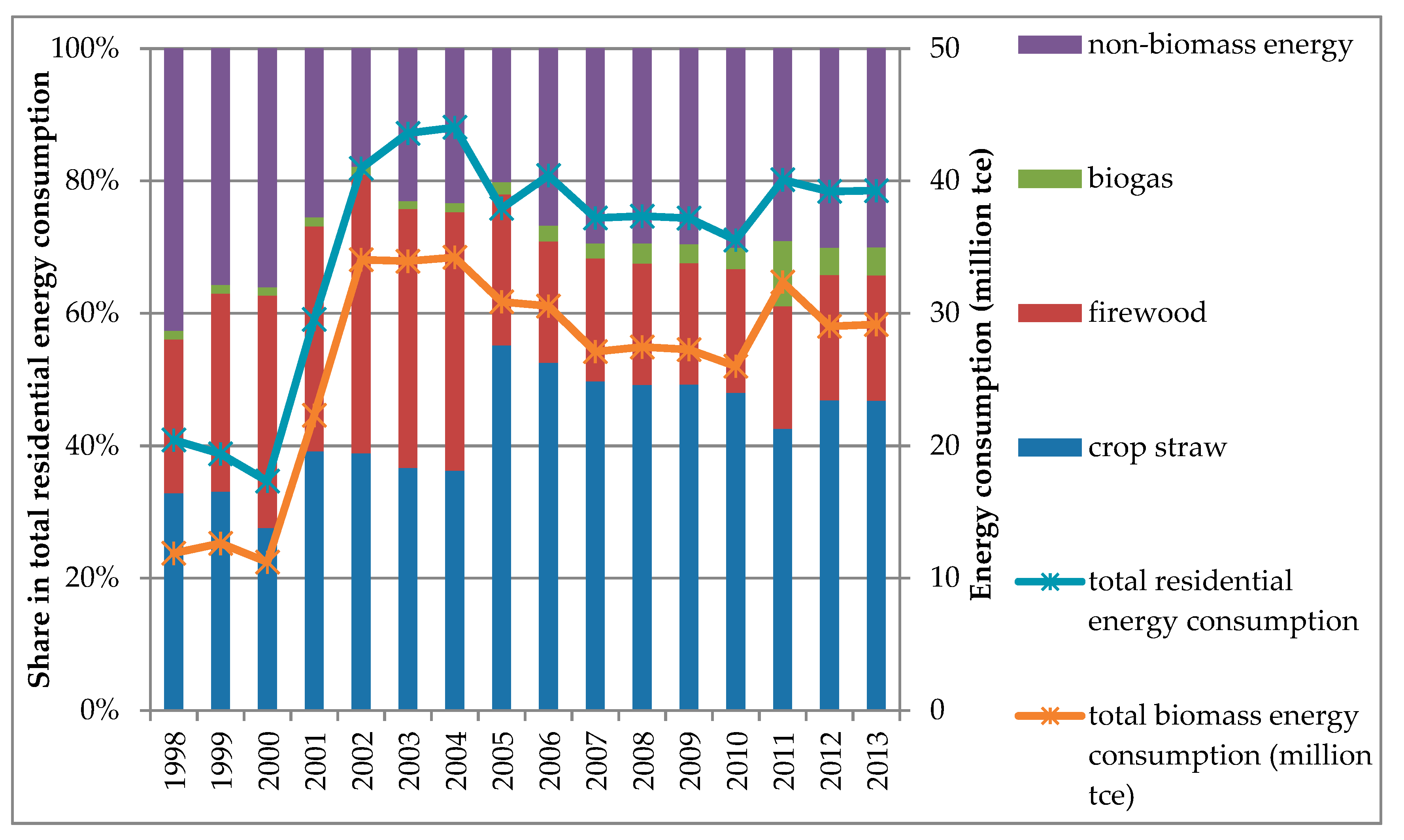
19]. In particular, biomass energy (In this paper, biomass energy is defined as crop straws collected after harvesting, firewood gathered from forestry and biogas mainly produced from pig dung, while commercial energy refers to those energy sources that can be purchased in the market.) is still the principal type of energy utilized for living purposes such as cooking and heating, accounting for around 42% of the total rural residential energy consumption in China [19]. Using biomass energy in the traditional way (i.e., direct combustion of crop straws and firewood in open air) not only lowers energy efficiency, but also destroys the rural environment [20]. Thus, in-depth analysis of the effects of urbanization on rural residential energy consumption, especially on biomass energy intensity, is necessary for providing policy implications on further promotion of the energy transition from traditional biomass energy (i.e., crop residues and firewood) to the advanced energy sources and sustainable development of the rural economy in China.
As little attention has been paid to the influences of urbanization on rural residential energy consumption and its related CO2 emissions in past investigations and few studies in China have focused on this issue at the city level due to data unavailability, the main research objective of this paper is to advance the literature by examining the effects of urbanization on energy intensity in the rural residential sector with the data from 21 prefectural-level cities in Sichuan Province of China. Herein, this paper focuses solely on the case of Sichuan Province in order to reduce the heterogeneities brought about by the variations in climatic and environmental conditions, economic development levels, and cultural and traditional factors across different stages of social development among provinces of China. Furthermore, since most of the rural areas in Sichuan Province are less developed compared to the general level of the whole country, the conclusions and policy implications of this study, to some extent, can be applied to other less developed regions in the world.
The rest of this paper is organized as follows. In Section 2, the mechanism by which urbanization is expected to affect rural residential energy consumption and CO2 emissions is presented. Section 3 provides the research methodology. The statistic information about urbanization, structural change in rural residential energy consumption and CO2 emissions in Sichuan Province, and the data used in this paper are described in Section 4. Section 5 reports and discusses the model estimation results. Section 6 concludes the main findings of this research and proposes some important policy implications for future energy development in rural China.

2. Theory and Hypothesis

Although urbanization is often studied in the context of economic development, it is a demographic indicator that promotes the shift of population concentration from rural to urban settings and changes human behaviors, thereby influencing household energy-using patterns [21]. Nevertheless, as urbanization is a complex dynamic process, the extent to which it affects rural residential energy consumption and its CO2 emissions has not been fully and clearly clarified in a single theory so far. Instead, the possible influences of urbanization on biomass energy use and energy-related CO2 emissions in the rural residential sector are partially discussed based on three basic outcome measurements of urbanization in the existing literature: population concentration, economic modernization and land use change.

2.1. The Effects of Population Concentration on Rural Residential Biomass Energy Consumption and CO2 Emissions

Although rural-to-urban migration is a significant driver of urbanization in the developing world, rapid urbanization reversely causes large-scale migration, resulting in a concentration of population and economic activity in urban areas [22]. One on hand, a reduction in rural population size decreases the total residential energy consumption and its CO2 emissions [23]. On the other hand, the changes in rural family structure can alter household energy using behaviors, especially on biomass energy consumption. In the context of migration, the well-educated younger generations are inclined to leave farms for a better future career, leaving a large rural population with a low education level and poor technical qualifications [24]. Moreover, the proportion of elderly people and children in rural families is also increasing. As a consequence, the total use of residential energy decreases with a degradation in energy consumption structure [20]. In other words, the share of biomass energy consumption in rural total residential energy consumption increases. In addition, urbanization builds strong and effective linkages between rural and urban areas through employment, consumption, marketing, transportation, and other ancillary services [25]. The new concepts on lifestyles and consumption patterns could be delivered back to rural areas by the newly urbanized citizens who prefer to use certain energy-intensive products such as small electrical devices and private vehicles, promoting the residential energy transition from traditional solid biomass energy to the advanced energy sources (e.g., electricity) [26,27].
To summarize, the effects of population changes induced by urbanization on total residential energy consumption are negative, while those effects on CO2 emissions and biomass energy consumption are ambiguous as the existing evidences on how residential energy consumption structural changes respond to the population changes are still insufficient. Thus, the first contribution of this paper is to investigate the influences of rural population size on residential energy consumption and CO2 emissions, with a particular focus on biomass energy consumption by testing the following hypothesis:
Hypothesis 1.
The decreasing rural population in the process of urbanization will reduce residential energy consumption and its related CO2 emissions in the residential sector, and it will push the progress of rural energy modernization by decreasing traditional biomass energy use.

2.2. The Effects of Economic Modernization on Rural Residential Biomass Energy Consumption and CO2 Emissions

Urbanization is usually associated with economic growth and the rapid process of industrialization. Under the dual-economy structure, urbanization can influence rural residential energy use and its CO2 emissions through direct and indirect channels. Many studies have indicated that residential energy consumption grows with the increase in income per capita caused by urbanization [28,29]. The plausible reason for this could be that the increasing disposable income enables rural residents to afford modern energy sources and increases the likelihood for them to purchase more electrical appliances [27,28]. Considering the changes in energy consumption structure, urbanization improves rural living standards by increasing the consumption of clean and high-efficiency energy such as natural gas and electricity. Accordingly, the energy-related CO2 emissions decrease [30].
Turning to the indirect channels by which urbanization impacts rural residential biomass energy consumption, industrialization can be defined as a process that a society transforms itself from a traditional agricultural society to one based on higher value-added manufacturing [27]. The result is the adjustment of the industrial structure (the share of value added of agriculture in GDP decreases, while that of the industrial sector in GDP increases) in rural areas and higher employment in non-agricultural sectors (especially in labor-intensive and service industries) [26,31]. The relationship between industrialization and rural residential energy consumption has been found to follow an inverted U-shape by many scholars [32,33,34]. Their findings revealed that industrialization narrows the urban-rural gap by boosting the rural economy and offering a large number of off-farm job opportunities to farmers so that it increases energy consumption to a peak value. And then, with the further acceleration of urbanization, structural changes at the industrial level and technical innovation increase energy using efficiency, which in turn, decreases residential energy consumption [35]. Regarding biomass energy consumption, it decreases due to the shrinking agriculture resulting from fast industrialization.
The conflicting results provided in existing studies have suggested that the relationship between urbanization, energy consumption and CO2 emissions is complex, since the effects of economic growth and industrialization on total amount of residential energy consumption and energy consumption structure have not been clarified. Thus, another contribution of this paper is to clarify the impacts of economic modernization on residential energy consumption and its CO2 emissions, with consideration of the changes in biomass energy consumption. Thus, the second basic hypothesis of this paper is:
Hypothesis 2.
Urbanization increases rural residential energy consumption and CO2 emissions through increasing the rural income level and the share of value-added of the industrial sector in GDP and non-agricultural employment, while decreasing biomass energy consumption through transforming the agriculture-based society to one based on other industries with higher value-added.

2.3. The Effects of Land Use Change on Rural Residential Biomass Energy Consumption and CO2 Emissions

Urbanization includes a spatial dynamic process of centralizing production factors to urban areas. This means that urbanization inevitably expands the city size and leads to land use change through land expropriation or occupation. Previous researches have indicated that land change use influences rural residential energy consumption and CO2 emissions mainly in two ways [26]. Firstly, the decrease in the area of arable land reduces agricultural production and the landless farmers are more likely to find jobs in nearby cities to increase their incomes. Hence, the total consumption of residential energy increases, while the consumption structure upgrades with a decreasing share of biomass energy [36]. Besides, land use changes for the construction of infrastructures, public services and facilities such as roads, stores and schools also raises the energy consumption in the residential sector [37,38]. On the contrary, if the speed of land urbanization exceeds that of population urbanization, the landless famers who are still left behind in rural areas will lose the indispensable resources for agricultural production and remain trapped in poverty. As a result, their energy consumption decreases and the available biomass resources for their residential energy use derived from agricultural production reduces at the same time [39].
Whereas the effects of land use change in the process of urbanization on rural residential energy consumption and CO2 emissions are still inconclusive, the biomass energy consumption is supposed to be negatively affected by the reduction of arable land caused by urbanization. Thus, the third contribution of this paper is to examine how land use change between urban–rural areas impacts residential energy consumption and its CO2 emissions. The hypothesis can be given as:
Hypothesis 3.
Urbanization reduces biomass energy consumption by decreasing the area of arable land, while simultaneously increasing the consumption of commercial energy to improve rural living qualities and conditions.
Based on these hypotheses, this paper investigates the different channels through which urbanization could impact residential energy intensity and CO2 emissions. Furthermore, the potential influencing mechanisms described in the three hypotheses also form the basis of the model specification and provide the selection criteria for variables used in the model estimation in the following empirical work of this paper.

3. Method

In previous literature, a large number of studies have investigated the effects of economic activities and demographic factors on energy consumption or environment using the IPAT model proposed by Ehrlich and Holdren (1971) [40]. The IPAT model can be written as follows:
I = P A T
In this model, the impact denoted by I is defined as the product of population size P , per capita affluence A (usually expressed in terms of GDP per capita), and technological factor T (such as the impact on environment per unit of GDP). The main limitation of the IPAT model is the over-simplification of the complex problem of energy consumption and the restriction of elasticities of energy consumption to unity [41,42,43]. Therefore, the IPAT model was later reformulated into the STIRPAT model as follows, in which more factors can be included into the model to account for the complex energy consumption pattern and variable elasticities of energy consumption can be modeled [44]:
E I i t = a i P i t α 1 A i t α 2 T i t α 3 e x p ( ε i t )
where a i represents the heterogenous individual effect. In model (2), we proxy energy consumption by energy intensity (EI). Rather than the unitary elasticity in the IPAT model, α 1 , α 2 and α 3 are respectively the elasticities of changes in P, A and T on environment or energy consumption to be estimated. ε i t denotes the disturbance term, subscript i (i = 1,…,N) represents the unit of analysis (prefectural-level cities) and t represents time. By taking natural logarithms to both sides of Equation (2), we can get:
ln E I i t = ln a i + α 1 ln ( P i t ) + α 2 ln ( A i t ) + α 3 ln ( T i t ) + ε i t
Unlike the original IPAT identity, multiple factors which were used to describe T can be included into the STIRPAT model [42]. Several studies used various indicators of urbanization to represent T in the STIRPAT model and estimated its impacts on energy use or energy intensity [1,4,8,10,45]; therefore, in model (4) we replace T with a vector of urbanization indicators URBAN to estimate its effect on energy consumption.
The dependent variable of model (3) refers to either total residential energy intensity (EIe), traditional biomass energy intensity (EItb), biogas intensity (EIg), or non-biomass energy intensity (EInb) (Energy intensity measures the energy requirement per unit of a driving economic variable. It is an indicator of the energy inefficiency of an economy. High energy intensities indicate a high price or cost of converting energy into GDP. In non-productive energy-consuming sectors (e.g., residential or household sector), GDP can be used as the driving economic variable [46]. It is a relative indicator measuring the dependence of rural economic growth on energy consumption. In this paper, it is calculated as a ratio of energy consumption to economic output (GDP)). Corresponding to the three potential impact channels of urbanization described in Section 2, in model (3) we use three groups of variables to represent URBAN: (1) population concentration in urban areas can be measured by the changes in rural population (P) and urbanization rate (UR); (2) economic modernization can be reflected by income level (A), industrialization rate (IND) and non-agricultural employment rate (NAE); (3) land use change is proxied by the area ratio of central urban zones to cultivated land (RL). In order to further investigate the impacts of urbanization on CO2 emissions, the following econometric model is also created based on rearranging the logarithm form of the STIRPAT model:
ln C E i t = β 1 ln E I i t + β 2 i ln ( P i t ) + β 3 ln ( A i t ) + β 4 ln ( U R B A N i t ) + σ i + μ i t
ln C E i t = δ k ln ( E I k i t ) + θ 1 ln ( P i t ) + θ 2 ln ( A i t ) + θ 3 ln ( U R B A N i t ) + π i + ω i t
where σ i and π i denote city-specific effects, and μ i t and ω i t represent stochastic error terms respectively. In model (4) and (5), the dependent variable in both models, CE, denotes the total amount of CO2 emissions from direct residential energy consumption. As mentioned in Section 2, urbanization affects CO2 emissions through influencing both the total amount and the structure of residential energy consumption. Hence, to identify these effects, denotes total residential energy intensity (EIe), while EIk represents the intensities of three different energy categories (i.e., traditional biomass energy (EItb), biogas (EIg) and non-biomass energy (EInb)) which are respectively included in the two models. Besides, the other variables on the right-hand side of model (3–5) are the same. Considering data availability and model simplification, the assumption of homogenous slope coefficients is made for model (3–5) [8,45].

4. Study Region and Data

4.1. Urbanization, Rural Residential Energy Consumption and CO2 Emissions in Sichuan Province

Sichuan Province is located in Southwestern China. It consists of 21 prefectural-level cities. In recent years, with deepening of the economic reform in China, rapid urbanization is an inevitable trend for rural development in Sichuan Province. According to the statistics, the urbanization rate increased dramatically from 18% in 1998 to 45% in 2013. Figure 1 shows the Sichuan cities map and geographic location of Sichuan province in China.
Currently, in Sichuan Province, the rural residential energy consumption still depends on traditional biomass energy generated from crop residues and firewood, due to the slow progress of energy transition towards modern energy [20]. By the end of 2013, the proportion of biomass energy (namely crop straws, firewood and biogas) in rural residential energy consumption was approximately 70% [20]. Figure 2 demonstrates the changes in the residential energy consumption structure of rural Sichuan Province between 1998 and 2013. As it is shown in Figure 2, the total residential energy consumption declined slightly from 20.43 million tce (tce = ton coal equivalent) in 1998 to 17.33 million tce in 2000. It then increased sharply to 44.04 million tce in 2004 and remained relatively stable around 38.24 million tce afterwards. Similarly, the total consumption of biomass energy was on average 11.91 million tce during the period between 1998 and 2000. It tripled from 11.21 million tce in 2000 to 34.23 million tce in 2004 and remained relatively steady at approximately 27.49 million tce from 2005 onwards. Moreover, traditional biomass energy (i.e., firewood and crop straw) takes the largest share in residential energy consumption. Although biogas holds a rather small share, the total proportion of biomass energy consumption peaked in 2002 with an average value of about 71%.
Figure 3 reflects the CO2 emissions from rural residential energy consumption in Sichuan Province from 1998 to 2013. It is illustrated in Figure 3 that the trend of the changes in CO2 emissions is similar to that of the changes in residential energy consumption, implying that the CO2 emissions are determined by total residential energy consumption. It can also be seen from Figure 3 that in most years, non-biomass energy consumption is accountable for more than half of the CO2 emissions in Sichuan Province. In addition, following a downward trend from 31.47 million tons in 1998 to 25.26 million tons in 2000, the total amount of CO2 emissions doubled to 53.73 million tons in 2004 and fluctuated thereafter until reaching 52.03 million tons in 2013. Moving to the CO2 emissions from biomass energy consumption, it steeply grew from 8.66 million tons in 2000 to 25.95 million tons in 2002 and kept around 21.88 million tons during the period from 2003 to 2013 with slight fluctuations.

4.2. Data Description

The data set used in this paper is a strictly balanced panel of 21 prefectural level cities in Sichuan Province covering the period 2006–2013. The data on rural energy consumption including consumption amounts of traditional biomass energy (crop straw and firewood), biogas and non-biomass energy are collected from the Rural Energy Office of Sichuan government (SCREO). The other original data are all collected from Sichuan Statistic Yearbooks (2007–2014).
The definitions of the variables used in the following empirical analysis are listed in Table 1. The CO2 emissions (CE) from direct residential energy consumption are calculated using the carbon-emissions-coefficient method (CECM) [4] (The calculation formula is: C E t = 44 12 × n = 1 N E C n t × c e f n × c o r n , where C E t represents the total CO2 emissions from residential energy consumption in year t; ECnt is the consumption amount of fuel type n (unit: million tce) in year t; cefn denotes the carbon emission coefficient of fuel type n (unit: ton per tce); and corn is the rate of carbon oxidation of fuel type n.). The intensity of energy is measured by energy consumption per real GDP, while the income level is measured as rural net income per capita (NIPC). IND is calculated as the ratio of industrial value added to GDP. Three other indicators are chosen to measure urbanization as follows. First, the percentage of the urban population in total population is computed as UR. A higher urbanization rate is usually associated with a higher urbanization degree. Second, the number of rural workers employed in the non-agricultural sector is divided by total employment to get NAE. With a fast urbanization, non-agricultural employment of rural labor increases as a result of industrial structural change and population concentration. Finally, the area ratio of central urban zones to cultivated land (RL) is taken to reflect the land use change in the process of urbanization. Urbanization drives conversion from cultivated land to urban central built-up areas [47] (As suggested by previous researches, the indicator of the percentage of the total agricultural area that has changed to artificial surfaces compared to a reference period is usually selected as the measurement of land use change from the agricultural sector to non-agricultural sector. However, due to data availability in China, this paper uses RL as a proxy). The area ratio of the two land cover types, therefore, increases.
Table 2 presents the summary statistics of the variables. For the natural logarithm value of the variables, the ratio of land use (RL) has the largest variability, while the urbanization rate (UR) has the smallest. For the complete panel of all the cities, during the period of 2006–2013, the average annual growth rates in intensities of total residential energy, traditional biomass energy, biogas, and non-biomass energy are negative at −19.4%, −21.5%, −26.1% and −15.7%, respectively. The total CO2 emissions (CE) and rural population (POP) decreased by 1.7% and 1.5% on average per year, while income level, industrialization rate, urbanization rate, ratio of land use, and non-agricultural employment rate increased by respectively 13.0%, 3.9%, 3.7%, 6.3%, and 2.0% per year, during the same period.

5. Results and Discussions

In order to investigate the relationship among urbanization, energy intensities and CO2 emissions, the empirical analysis is conducted by estimating models (3–5) (Firstly, for the energy intensity models in Equation (3), standard panel regression techniques including pooled ordinary least squares (POLS), fixed effects (FE), first differences (FD), and fixed effects with instrumental variables (FE-IV) are used. Four types of energy intensity are investigated, namely total residential energy intensity (EIe), traditional biomass energy intensity (EItb), biogas intensity (EIg), and non-biomass energy intensity (EInb). Table 3, Table 4, Table 5 and Table 6 report a series of estimated results for the energy intensity models with each column specified by these four different panel regression methods. POLS is initially run on panel data. Given the heterogeneity in the sample, the FE and FD estimations are applied to alleviate the unobserved heterogeneity bias caused by time-invariant omitted variables. However, by using the Wooldridge test for autocorrelation in panel data [48], serial correlation is found in the residuals from all FD regressions as shown in the last column of each table. This implies that for all models, the FE estimators are more efficient than the FD estimators. Nevertheless, when the assumption of ‘strict exogeneity’ fails (In Equation (3), the potential endogeneity problem is caused by the correlation between energy intensities (EI) and net income capita (NIPC), as GDP and NIPC are highly correlated. We also use Hausman test to check the endogeneity of NIPC. The statistic of the Hausman test in Table 3, Table 4, Table 5 and Table 6 implies that NIPC should be treated as an endogenous variable in each model of Equation (3)), both FE and FD are biased. In this case, instrumental variables (IV) are included in model specification.
On the other hand, in terms of the goodness of fit of each model, two other attributes of residuals, cross-sectional dependence and stationarity should be considered in order to obtain a more accurate estimate [45]. Since the presence of cross-sectional dependence in the residual is viewed as a consequence of model misspecification, classic panel unit root tests that do not take cross-sectional dependence into account can be misleading (have low power) [49,50,51]. Therefore, the Cross-section Dependence (CD) test and Cross-sectional Im-Pesaran-Sin (CIPS) test are adopted to check for cross-sectional independency and stationarity in residuals [52,53,54]. According to the test results presented in Table 3 and Table 4 (residential energy intensity and traditional biomass energy intensity models), only the FE-IV estimators perform well because the high p-values associated with the CD test suggest little evidence of cross-sectional dependence in residuals from the FE-IV regressions, and the rejections of the null hypotheses for the CIP test indicate that the FE-IV regressions are well fitted with stationary residuals. In the case of the biogas intensity model (See Table 5), the CD test reveals the problem of cross-sectional dependence in all specifications, while the CIPS test demonstrates that all estimation results suffer from non-stationary residuals (In this case, the FE-IV specification is relatively better because it addressed the problem caused by the endogenous explanatory variable NIPC). In addition, for the non-biomass energy intensity model (See Table 6), although the CD test results continue to show that there is an issue with cross-sectional dependence, the FE-IV and POLS estimators are more reliable as the CIP test results reflect that they have stationary residuals.
In summary, the estimated coefficients of the FE-IV regressions are preferred for interpretation of the estimation results of the energy intensity models, as they properly address the important econometric concerns including heterogeneity bias, endogeneity, residual cross-sectional dependence, and residual non-stationarity. Hence, our main discussions in this study will focus only on the FE-IV models.
Table 3 lists the estimated effects of urbanization on total rural residential energy intensity, while Table 4, Table 5 and Table 6 illustrate the effects on the intensities of traditional biomass energy, biogas and non-biomass energy, respectively. As it is shown in Table 3, the estimated coefficients of the FE-IV specification reveal that net income per capita, rural population and ratio of land use can significantly and negatively affect total residential energy intensity, while urbanization has a significantly positive impact on it. According to the magnitudes of the coefficients, a 1% increase in net income per capita, rural population, and ratio of land use decreases rural residential energy intensity by 1.15%, 1.46% and 0.76% respectively, whereas a 1% increase in urbanization rate increases it by 1.46%. Additionally, although the estimated coefficients on industrialization rate and non-agricultural employment are not statistically significant in the FE-IV specification, the signs of them are the same in all specifications. This means that industrialization negatively influences residential energy intensity, while non-agricultural employment has a positive effect on it. However, these effects are insignificant.
Table 4 reveals that the effects of net income per capita and rural population on traditional biomass energy intensity are significantly negative in all specifications. Concretely, the FE-IV estimators suggest that a 1% decrease in rural population increases traditional biomass energy intensity by 1.61%, while a 1% increase in net income per capita will reduce the intensity of traditional biomass energy consumption by 1.26%. The results of this model also show that the impacts of urbanization rate and ratio of land use on traditional biomass energy intensity are statistically significant at the 5% level and 1% level, but have opposite signs. A 1% increase in urbanization rate increases traditional biomass energy intensity by 1.68%, while a 1% increase in the ratio of land use reduces the intensity by 0.83%.
For the case of biogas use (See Table 5), the estimated coefficients of rural population and industrialization rate are positive and statistically significant at the 1% level in the FE-IV model. A 1% decrease in rural population decreases biogas intensity by 4.32%, while a 1% increase in industrialization rate increases the intensity of biogas use by 1.05%. Besides, non-agricultural employment also has a positive but insignificant impact on biomass intensity.
Similarly, regarding non-biomass energy intensity, it can be seen from Table 6 that the estimated coefficients net income per capita, industrialization rate and ratio of land use have significant and negative effects on non-biomass energy intensity, while the urbanization rate significantly and positively influences the intensity of non-biomass energy use. The elasticity of non-biomass energy intensity to net income per capita is −0.84, while the elasticity to urbanization rate is 1.43. A 1% increase in industrialization rate and ratio of land use reduces non-biomass energy intensity by 0.30% and 0.87%, respectively.
Likewise, the two CO2 emission models specified in Equations (4) and (5) are estimated using the same estimation techniques, namely POLS, FE, FD, and FE-IV (As little evidence of endogeneity is shown in the statistics of the Hausman test (See Table 7 and Table 8); NIPC in the CO2 emission models can be regarded as exogenous variables. In this case, the FE-IV estimators are included in the CO2 emissions). Table 7 presents the impacts of urbanization on total residential energy use and its CO2 emissions, while Table 8 reflects the indirect effects of urbanization on CO2 emissions occurring through the changes in energy consumption structure (i.e., in the intensities of three energy categories). It should be noted that the estimation results of the CO2 emission models are not robust. This can possibly be attributed to the applied estimation approaches and data. The results of the Wooldridge test for autocorrelation in panel data indicate that for both of these two models, the FE estimators are more efficient than the FD estimators. Nevertheless, the results of the CD and CIPS tests show that the FD estimators are more reliable.
More specifically, in Table 7, the estimated coefficient on total residential energy intensity is positive and statistically significant at the 1% level in each specification. It ranges from 0.323 to 0.580. The estimated coefficients of net income per capita and urbanization rate are positive, but not statistically significant in all specifications. Collectively, these results suggest that increases in total residential energy intensity increase CO2 emissions, whereas net income per capita and urbanization rate have statistically insignificant influences on CO2 emissions. The estimated coefficient on non-agricultural employment is statistically significant in each specification. It is positive and covers a fairly tight range between 0.227 and 0.282 in the FE, FD and FE-IV specifications, indicating that raising non-agricultural employment increases CO2 emissions (As the POLS estimators suffer from the heterogeneity bias, the FE, FD and FE-IV estimators are more preferred for interpreting the model estimation results). In addition, for the rural population, industrialization rate and ratio of land use, the signs of their coefficients are different and only statistically significant in one or two of the four specifications, demonstrating that the estimated coefficients of these variables are more sensitive to the estimation technique than the estimated coefficients of the other variables.
Empirical results for the CO2 emission model with the intensities of three energy categories are provided in Table 8. The estimated coefficient on the intensity of traditional biomass energy is statistically significant in each specification at the 1% level and ranges in value between 0.150 and 0.295. The estimated coefficients on non-biomass energy intensity and urbanization rate are positive and statistically significant in three out of the four specifications. More specifically, the estimated coefficient of non-biomass energy intensity ranges from 0.063 to 0.362, while that of the urbanization rate ranges from 0.457 to 1.128. The estimated coefficient of net income per capita is positive but statistically insignificant in two specifications. These results indicate that the use of traditional biomass energy contributes the most to CO2 emissions. Reducing the intensity of traditional biomass energy can decrease CO2 emissions. Besides, the signs of the parameters on the other variables depend on the adopted estimation methods.
Furthermore, the model estimation results listed in Table 3, Table 4, Table 5, Table 6, Table 7 and Table 8 also allow to test the three aforementioned hypotheses (in Section 2) by identifying how the different measurements of urbanization directly and indirectly impact energy intensities and CO2 emissions via three channels (namely population concentration, economic modernization and land use change). The direct effects come from the changes in the total amount of residential energy consumption, whereas the indirect effects occur through the variations in energy consumption structure.
Hypothesis 4:
the effects of population concentration on residential energy intensity and CO2 emissions.
According to the estimation results, rural population significantly and negatively influences the intensity of rural residential energy, whereas the relationship between urbanization rate and residential energy intensity is positive and statistically significant. In terms of the real situation of China, as the large-scale urban–rural migration caused by urbanization usually results in declines in rural population and increases in urbanization rate at the same time, the findings of this paper also indicate that population concentration in urban areas is associated with an increase in total residential energy intensity and its related CO2 emissions. Regarding the different types of residential energy sources, rural population has a negative and statistically significant impact on traditional biomass energy intensity, while it positively influences biogas intensity. Moreover, the urbanization rate has a positive and statistically significant influence on the intensities of traditional biomass energy and non-biomass energy. These results may be due to the changes in the structure of rural family. Since the proportion of elderly people and children increases, the using efficiency of residential energy decreases and the dependency on traditional biomass energy for living increases. Thus, total residential energy intensity increases in the process of urbanization with increases in the intensities of traditional biomass energy and non-biomass energy.
In short, this paper provides insufficient evidence to support Hypothesis 4 that a decrease in rural population will decrease total residential energy consumption and its related CO2 emissions. On the contrary, population concentration has a positive and statistically significant impact on total residential energy intensity and CO2 emissions, as it can positively and significantly influence traditional biomass energy intensity and non-biomass energy intensity.
Hypothesis 5:
the effects of economic modernization on residential energy intensity and CO2 emissions.
In this paper, the economic modernization is measured by net income per capita, industrialization rate and non-agricultural employment rate. It can be seen from the estimation results that net income per capita is an important factor impacting residential energy use. Generally, it significantly and negatively affects total residential energy intensity. In other words, raising the income level in rural areas can decrease the intensity of residential energy use. The plausible reason for this could be that the increase of income enables rural residents to pay for energy sources with higher efficiency. The model estimation results also show that net income per capita can negatively influence the intensities of traditional biomass energy and non-biomass energy. Although insufficient evidence has been presented in this paper to support a significant relationship between biogas intensity and income level, the total effects of income per capita on biomass energy intensity should be negative due to the rather small share occupied by biogas in total rural residential energy consumption.
The industrialization rate can be regarded as another influencing factor for energy intensities. The strongest evidence comes from the FE-IV regression for non-biomass energy intensity, as the estimated coefficient on industrialization rate is negative and statistically significant in it. The main reason could be that rapid industrialization promotes technical innovation for increases in using efficiency of non-biomass energy such as coal, natural gas and electricity. Moreover, the industrialization rate has a statistically significant and positive influence on biogas intensity. This phenomenon could occur as industrialization pushes forward the economic growth in rural areas, so that the process of energy transition from traditional solid biomass energy to more efficient biofuels (i.e., biogas) accelerates. The demand for rural economic development for biogas therefore increases. Similarly, in this case, the aggregate effects of the industrialization rate on biomass energy intensity should also be negative.
The estimated coefficient of the non-agricultural employment rate is positive in all energy intensity models, though it is statistically insignificant. This provides evidence for believing the correlations between non-agricultural employment and energy intensities are likely to be positive. The possible reason for this could be that non-farm employment increases the total amount of residential energy consumption by boosting the rural economy. To sum up, the study results of this paper can only provide limited information for testing Hypothesis 5. Economic modernization promoted by urbanization could reduce total residential energy intensity and CO2 emissions, as net income per capita has a negative effect on rural residential energy intensity, especially on the intensities of traditional biomass energy and non-biomass energy. Moreover, industrialization could improve the using efficiency of residential energy particularly through increasing that of non-biomass energy, which in turn, decreases the demand of rural economic growth for energy in rural residential sector. Hence, the total residential energy consumption and its CO2 emissions will decline with a rapid industrialization. This is inconsistent with Hypothesis 5.
Hypothesis 6:
the effects of land use change on residential energy intensity and CO2 emissions.
The estimated coefficients on the area ratio of central urban built-up zones to cultivated land are significantly negative in the models of total residential energy intensity, traditional biomass energy intensity and non-biomass energy intensity, implying that the conversion of agricultural land to non-agricultural use reduces total residential energy intensity by decreasing the intensities of traditional biomass energy and non-biomass energy. The underlying reason for these results could be that the shrink of arable land decreases agricultural production, thereby reducing the amount of biomass resources available for energy use. Moreover, landless farmers are more likely to find jobs in cities and to live there. Thus, the consumption of residential energy in rural areas, especially that of non-biomass energy, reduces. Accordingly, the related CO2 emissions decrease.
Hence, the results of this paper can partly support Hypothesis 6, that urbanization reduces biomass energy consumption for residential purposes as it decreases the area of arable land. In a nutshell, land use change with urbanization decreases total residential energy intensity. In particular, it simultaneously reduces the intensities of traditional biomass energy and non-biomass energy.

6. Conclusions

While there has been a lot of work on investigating the effects of urbanization on energy intensity and CO2 emissions, much less is known about how various indicators of urbanization affect intensities of different energy sources and related CO2 emissions in the rural residential sector in developing countries. The urban population is expected to increase rapidly in developing countries. The impact of urbanization on rural residential energy consumption structure and CO2 emissions deserves serious consideration. These issues have been explored in this paper by estimating a variety of panel data models using the standard econometric techniques and the data from Sichuan Province, China.
According to the estimation results of the energy intensity models, urbanization affects rural residential energy intensity through the direct and indirect channels. As a direct result of urbanization, population concentration measured by rural population and urbanization rate positively affects total residential energy intensity by increasing the intensities of traditional biomass energy and non-biomass energy. Indirectly, with respect to the three indicators of economic modernization in the process of urbanization, net income per capita is an important driver of reductions in energy intensity. It significantly and negatively affects total residential energy intensity and the intensities of traditional biomass energy and non-biomass energy. These results are consistent with previous studies that also employed China’s provincial level data [16,20,55,56]. The industrialization rate is another major influencing factor of the intensity of energy use in the rural residential sector. Although it has no statistically significant effect on total residential energy intensity, it negatively impacts non-biomass energy intensity and positively affects biogas intensity. This may be due to cleaner energy utilization benefiting from technology advancement. Besides, the findings of this paper also indicate that non-agricultural employment could have a positive but insignificant impact on energy intensities. In addition, land use change negatively and significantly influences the intensities of total residential energy, traditional biomass energy and non-biomass energy.
On the other hand, the estimation results of the CO2 emission models reveal that the estimated coefficient of total residential energy intensity is positive and statistically significant at the 1% level in each specification. The CO2 emission elasticities of residential energy intensity range from 0.323 to 0.580. These findings confirm that decreasing residential energy intensity can make contributions to climate change mitigation by reducing CO2 emissions. More specifically, traditional biomass energy accounts for most of the CO2 emissions from residential energy use as the estimated coefficient on it is also positive and statistically significant in each specification at the 1% level, and the coefficient ranges from 0.150 to 0.295. The relationship between the intensities of biogas and non-biomass energy and CO2 emissions could be positive but not robust. Relatively, it can be found that biogas use has a lower effect on CO2 emissions by comparing the magnitudes of the coefficients in each specification. The other measurements of urbanization present no consistent sign or significance in all specifications of both models. Nevertheless, the combined effect of increasing all urbanization measurements will lead to higher CO2 emissions. From a policy perspective, the findings of this paper suggest that reducing residential energy intensity, particularly the intensity of traditional biomass energy, is an effective way to mitigate the threat of climate change caused by CO2 emissions, while promoting biogas is another way to control CO2 emissions. Moreover, as the urbanization rate is expected to continually increase in China and many other developing countries, the CO2 emissions from rural residential energy consumption are correspondingly expected to increase. Under this circumstance, policies aiming at accelerating industrialization by upgrading industrial structure and technology will lead to a fall in the intensity of non-biomass energy such as coal, natural gas and electricity, which in turn will reduce CO2 emissions. Furthermore, raising the income level can not only reduce total residential energy intensity and its CO2 emissions, but also potentially optimize the energy consumption structure by decreasing the dependence of rural economic growth on traditional biomass energy and non-biomass energy in residential sector. There are a few limitations of our research. First, we only measured urbanization through indicators of population concentration, economic modernization, and land use change, environmental and ecological indicators of urbanization have mostly been ignored, so the analysis of urbanization on rural residential energy use and CO2 emissions are sort of incomplete. Secondly, due to data availability, we only included Sichuan Province in our study, it is needed to obtained more data to enhance the external validity of the conclusions in the future study.

Author Contributions

Conceptualization, Q.C. and H.Y.; Data curation, Q.C. and W.W.; Formal Analysis, Q.C.; Methodology, Q.C. and T.L.; Writing—original draft, Q.C.; Writing—review & editing, H.Y.

Funding

The research was funded by Hermann Eiselen Doctoral Programm of the Foundation of Fiat Panis, grant number PN30800138.

Acknowledgments

We are grateful for Wanlin He for his enthusiastic support and help in acquiring data. Financial support from SWUPL (Project No. E-7102-16-00004-0112) is acknowledged to make the collaboration between the co-authors possible.

Conflicts of Interest

The authors declare no conflict of interest.

References

  1. Poumanyvong, P.; Kaneko, S.; Dhakal, S. Impacts of urbanization on national transport and road energy use: Evidence from low, middle and high-income countries. Energy Policy 2012, 46, 268–277. [Google Scholar] [CrossRef]
  2. World Bank. World Development Indicator Database. Available online: https://data.worldbank.org/indicator/SP.RUR.TOTL.ZS?view=chart (accessed on 3 April 2019).
  3. UNDESA. 2018 Revision of World Urbanization Prospects. Available online: https://www.un.org/development/desa/publications/2018-revision-of-world-urbanization-prospects.html (accessed on 16 May 2018).
  4. Wang, Q.; Wu, S.D.; Zeng, Y.E.; Wu, B.W. Exploring the relationship between urbanization, energy consumption, and CO2 emissions in different provinces of China. Renew. Sustain. Energy Rev. 2016, 54, 1563–1579. [Google Scholar] [CrossRef]
  5. Poumanyvong, P.; Kaneko, S. Does urbanization lead to less energy use and lower CO2 emissions? A cross-country analysis. Ecol. Econ. 2010, 70, 434–444. [Google Scholar] [CrossRef]
  6. Guo, W.; Sun, T. Impact of urbanization on regional energy consumption and residents’ energy consumption in China. China Environ. Sci. 2015, 35, 3166–3176. [Google Scholar]
  7. Jiang, Z.J.; Lin, B.Q. China’s energy demand and its characteristics in the industrialization and urbanization process. Energy Policy 2012, 49, 608–615. [Google Scholar] [CrossRef]
  8. Sadorsky, P. Do urbanization and industrialization affect energy intensity in developing countries? Energy Econ. 2013, 37, 52–59. [Google Scholar] [CrossRef]
  9. Ribeiro, K.S.; Kobayashi, S.; Beuthe, M.; Gasca, J.; Greene, D.; Lee, D.S.; Muromachi, Y.; Newton, P.J.; Plotkin, S.; Sperling, D.; et al. Transport and its infrastructure. In Climate Change 2007: Mitigation-Contribution of Working Group III to the Fourth Assessment Report of the Intergovernmental Panel on Climate Change; Metz, B., Davidson, O., Bosch, P.R., Dave, R., Meyer, L.A., Eds.; Cambridge University Press: Cambridge, UK, 2008. [Google Scholar]
  10. Salim, R.; Rafiq, S.; Shafiei, S. Urbanization, Energy Consumption and Pollutant Emission in Asian Developing Economies: An Empirical Analysis; ADBI Working Paper Series: Tokyo, Japan, 2017. [Google Scholar]
  11. Jones, D.W. How urbanization affects energy-use in developing countries. Energy Policy 1991, 19, 610–630. [Google Scholar] [CrossRef]
  12. Fan, J.L.; Zhang, Y.J.; Wang, B. The impact of urbanization on residential energy consumption in China: An aggregated and disaggregated analysis. Renew. Sustain. Energy Rev. 2017, 75, 220–233. [Google Scholar] [CrossRef]
  13. Ganesan, P.; Thirugnanasambandam, M.; Rajakarunakaran, S.; Devaraj, D. Specific energy consumption and CO2 emission reduction analysis in a textile industry. Int. J. Green Energy 2015, 12, 685–693. [Google Scholar] [CrossRef]
  14. Hao, Y.; Huang, Y. Exploring the nexus of energy consumption structure and CO2 emission in China: Empirical evidence based on the translog production function. Pol. J. Envion. Stud. 2018, 27, 2541–2551. [Google Scholar] [CrossRef]
  15. NBSC. China Energy Statistical Yearbook 2016; Science Press: Beijing, China, 2016. [Google Scholar]
  16. Zhang, C.G.; Lin, Y. Panel estimation for urbanization, energy consumption and CO2 emissions: A regional analysis in China. Energy Policy 2012, 49, 488–498. [Google Scholar] [CrossRef]
  17. The 13th Five-Year Plan for National Socio-Economic Development of China; Central Committee of the Communist Party of China (CCCPC): Beijing, China, 2015.
  18. State Council of PRC. Work Plan for Controlling Greenhouse Gas Emission during the 13th Five-Year Plan Period. Available online: http://www.gov.cn/zhengce/content/2016-11/04/content_5128619.htm (accessed on 23 April 2019).
  19. Qiu, H.G.; Yan, J.B.; Li, D.W.; Han, W. Residential energy consumption in rural China: Current situation and determinants for future trend: An empirical study based on field survey data of 4 provinces. China Soft Sci. 2015, 11, 28–38. [Google Scholar]
  20. Chen, Q.; Yang, H.R.; Liu, T.B.; Zhang, L. Household biomass energy choice and its policy implications on improving rural livelihoods in Sichuan, China. Energy Policy 2016, 93, 291–302. [Google Scholar] [CrossRef]
  21. Barnes, D.F.; Krutilla, K.; Hyde, W.F. The Urban Household Energy Transition: Social and Environmental Impacts in the Developing World; Routledge: Washington, DC, USA, 2005. [Google Scholar]
  22. Nauman, E.; Vanlandingham, M.; Anglewicz, P. Migration, Urbanization and Health. In International Handbook of Migration and Population Distribution; White, M., Ed.; Springer: Dordrecht, The Netherlands, 2016; Volume 6, pp. 1520–1525. [Google Scholar]
  23. Komatsu, S.; Ha, H.D.; Kaneko, S. The effects of internal migration on residential energy consumption and CO2 emissions: A case study in Hanoi. Energy Sustain. Dev. 2013, 17, 572–580. [Google Scholar] [CrossRef]
  24. Chen, Q.; Liu, T.B. Biogas system in rural China: Upgrading from decentralized to centralized? Renew. Sustain. Energy Rev. 2017, 78, 933–944. [Google Scholar] [CrossRef]
  25. Arshad, F.M.; Shamsudin, M.N. Rural Development Model in Malaysia. Available online: http://econ1.upm.edu.my/~fatimah/rural.pdf (accessed on 3 April 2019).
  26. Li, F.Q.; Sun, F.Y.; Cao, J.H. The mechanism of the effect of urbanization on rural life energy consumption: An empirical analysis based on 1997-2012 provincial panel data of China. Syst. Eng. 2016, 34, 70–75. [Google Scholar]
  27. Elliott, R.J.R.; Sun, P.Y.; Zhu, T. The direct and indirect effect of urbanization on energy intensity: A province-level study for China. Energy 2017, 123, 677–692. [Google Scholar] [CrossRef]
  28. Zhang, M.; Guo, F.Y. Analysis of rural residential commercial energy consumption in China. Energy 2013, 52, 222–229. [Google Scholar] [CrossRef]
  29. Nie, H.G.; Kemp, R.; Xu, J.H.; Vasseur, V.; Fan, Y. Drivers of urban and rural residential energy consumption in China from the perspectives of climate and economic effects. J. Clean. Prod. 2018, 172, 2954–2963. [Google Scholar] [CrossRef]
  30. Rosas, J.; Sheinbaum, C.; Morillon, D. The structure of household energy consumption and related CO2 emissions by income group in Mexico. Energy Sustain. Dev. 2010, 14, 127–133. [Google Scholar] [CrossRef]
  31. Ma, C.; Stern, D.I. China’s changing energy intensity trend: A decomposition analysis. Energy Econ. 2008, 30, 1037–1053. [Google Scholar] [CrossRef]
  32. Saboori, B.; Sulaiman, J.; Mohd, S. Economic growth and CO2 emissions in Malaysia: A co-integration analysis of the environmental Kuznets Curve. Energy Policy 2012, 51, 184–191. [Google Scholar] [CrossRef]
  33. Hao, Y.; Liao, H.; Wei, Y.M. The environmental Kuznets curve for China’s per capita energy consumption and electricity consumption: An empirical estimation on the basis of spatial econometric analysis. China Soft Sci. 2014, 1, 134–147. [Google Scholar]
  34. Ndoricimpa, A. Threshold effects of debt on economic growth in Africa. Afr. Dev. Rev. 2017, 29, 471–484. [Google Scholar] [CrossRef]
  35. Liao, H.; Fan, Y.; Wei, Y.M. What induced China’s energy intensity to fluctuate: 1997-2006? Energy Policy 2007, 35, 4640–4649. [Google Scholar] [CrossRef]
  36. Zhou, Y.; Liu, Y.; Wu, W.; Li, Y. Effects of rural-urban development transformation on energy consumption and CO2 emissions: A regional analysis in China. Renew. Sustain. Energy Rev. 2015, 52, 863–875. [Google Scholar] [CrossRef]
  37. Banuri, T.; Barker, T.; Bashmakov, I. Technical summary. In Climate Change 2001: Mitigation-Contribution of Working Group III to the Third Assessment Report of the Intergovernmental Panel on Climate Change; Metz, B., Davidson, O., Swart, R., Pan, J., Eds.; Cambridge University Press: Cambridge, UK, 2001; p. 762. [Google Scholar]
  38. Chawla, S. Land use changes in India and its impacts on environment. J. Environ. 2012, 1, 14–20. [Google Scholar]
  39. Wang, X.B.; Shao, Y.F. Research on energy consumption and carbon dioxide emissions in China’s urbanization: Empirical study based on the provincial panel data. Technoecon. Manag. Res. 2014, 7, 19–23. [Google Scholar]
  40. Ehrlich, P.R.; Holdren, J.P. Impact of population growth. Science 1971, 171, 1212–1217. [Google Scholar] [CrossRef]
  41. Dietz, T.; Rosa, E.A. Rethinking the environmental impacts of population, affluence and technology. Hum. Ecol. Rev. 1994, 1, 277–300. [Google Scholar]
  42. York, R.; Rosa, E.A.; Dietz, T. STIRPAT, IPAT and ImPACT: Analytic tools for unpacking the driving forces of environmental impacts. Ecol. Econ. 2003, 46, 351–365. [Google Scholar] [CrossRef]
  43. Martínez-Zarzoso, I.; Maruotti, A. The impact of urbanization on CO2 emissions: Evidence from developing countries. Ecol. Econ. 2011, 70, 1344–1353. [Google Scholar] [CrossRef]
  44. Dietz, T.; Rosa, E.A. Effects of population and affluence on CO2 emissions. Proc. Natl. Acad. Sci. USA 1997, 94, 175–179. [Google Scholar] [CrossRef]
  45. Ma, B. Does urbanization affect energy intensities across provinces in China? Long-run elasticities estimation using dynamic panels with heterogeneous slopes. Energy Econ. 2015, 49, 390–401. [Google Scholar] [CrossRef]
  46. Bhattacharyya, S.C. Energy Economics: Concepts, Issues, Markets and Governance; Springer: London, UK, 2011. [Google Scholar]
  47. Yao, X.W.; Wang, Z.Q.; Wang, H. Impact of Urbanization and Land-Use Change on surface climate in Middle and Lower Reaches of the Yangtze River, 1988–2008. Adv. Meteorol. 2015, 4, 395094. [Google Scholar] [CrossRef]
  48. Wooldridge, J.M. Econometric Analysis of Cross Section and Panel Data; MIT Press: Cambridge, UK, 2002. [Google Scholar]
  49. Baltagi, B.H. Analysis of Panel Data, 3rd ed.; John & Wiley, Ltd.: West Sussex, UK, 2005. [Google Scholar]
  50. Sarafidis, V.; Wansbeek, T. Cross-sectional dependence in panel data analysis. J. Economt. Rev. 2012, 31, 483–531. [Google Scholar] [CrossRef]
  51. Sadorsky, P. The effect of urbanization on CO2 emissions in emerging economies. Energy Econ. 2014, 41, 147–153. [Google Scholar] [CrossRef]
  52. Pesaran, M.H. Estimation and inference in large heterogeneous panels with a multifactor error structure. Econometrica 2006, 74, 967–1012. [Google Scholar] [CrossRef]
  53. Pesaran, M.H. A simple panel unit root test in the presence of cross-section dependence. J. Appl. Economet. 2007, 22, 265–312. [Google Scholar] [CrossRef] [Green Version]
  54. Pesaran, M.H. General Diagnostic Tests for Cross Section Dependence in Panels. Available online: http://ftp.iza.org/dp1240.pdf (accessed on 23 April 2019).
  55. Song, F.; Zheng, X. What drives the change in China’s energy intensity: Combining decomposition analysis and econometric analysis at the provincial level. Energy Policy 2012, 51, 445–453. [Google Scholar] [CrossRef]
  56. Jiang, L.; Former, H.; Ji, M. The drivers of energy intensity in China: A spatial panel data approach. China Econ. Rev. 2014, 31, 351–360. [Google Scholar] [CrossRef]
Figure 1. Map of Sichuan. Source: this map is produced by the authors by using the base map from China Highlits and China Discovery.
Sustainability 11 02421 g001
Figure 2. Rural residential energy consumption structure in Sichuan Province (1998–2013). Source: Data from 1998 to 2000 are collected from China Agriculture Statistical Report 1998, 1999 and 2000; data from 2001 to 2005 are collected from China Energy Statistical Yearbook 2000–2002, 2004, 2005 and 2006; data from 2006 to 2013 are collected from Compilation of Sichuan Rural Renewable Energy Statistics (2006–2013).
Sustainability 11 02421 g002
Figure 3. Structure of CO2 emissions from residential energy consumption (1998–2013). Source: Author’s own calculation based on the data collected from China Agricultural Statistical Report 1998, 1999 and 2000; China Energy Statistical Yearbook 2000–2002, 2004, 2005 and 2006; Compilation of Sichuan Rural Renewable Energy Statistics (2006–2013).
Sustainability 11 02421 g003
Table 1. Definition of the variables used in this study over the period 2006–2013.
VariableDefinition
EIeRatio of total residential energy consumption to GDP (Tce per ten thousand CNY 1)
EItbRatio of total traditional biomass energy consumption to GDP (Tce per ten thousand CNY)
EIgRatio of total biogas consumption to GDP (Tce per ten thousand CNY)
EInbRatio of total non-biomass energy consumption to GDP (Tce per ten thousand CNY)
CETotal CO2 emission from rural residential energy consumption (ten thousand ton)
NIPCRural net income per capita per year (CNY)
INDShare of industry sector in GDP
URThe percentage of total population living in urban area (%)
NAEThe percentage of total labor force employed in non-agricultural sector (%).
POPTotal rural population (10 thousand)
RLThe ratio of urban built-up area to cultivated land.
1 Tce (Tonne of coal equivalent), CNY (Chinese Yuan).
Table 2. Summary statistics.
ObsMeanSt.Dev.MinMax
EIe168−1.2230.615−2.7110.106
EItb168−1.5860.717−3.539−0.158
EIg168−4.7020.715−6.399−2.807
EInb168−2.7530.736−4.946−1.247
CE1685.2320.7163.3986.988
POP1685.4010.6363.7076.240
UR1683.581 0.262 2.885 4.240
NAE1683.4980.3981.8304.127
IND1683.7020.321 2.510 4.277
RL168−3.7130.857−5.480−1.247
NIPC1688.5120.4027.3019.472
Growth rate
EIe147−0.1940.223−1.4960.411
EItb147−0.2150.294−1.8500.536
EIg147−0.2610.760−2.8610.734
EInb147−0.1570.160−1.2660.411
CE147−0.0170.181−1.1290.433
POP147−0.0150.015−0.0760.030
UR1470.0370.023−0.0310.109
NAE1470.0200.149−1.2980.552
IND1470.0390.088−0.7670.319
RL1470.0630.086−0.2700.430
NIPC1470.1300.065−0.4470.508
Table 3. Effects of urbanization on residential energy intensity.
POLSFEFE-IVFD
NIPCa−0.744 *** (0.107)−0.789 *** (0.120)−1.150 *** (0.158)−0.564 ** (0.269)
POP−0.067 (0.054)−1.431 ** (0.663)−1.462 ** (0.739)−0.586 (0.508)
UR−1.847 *** (0.304)0.011 (0.458)1.464 *** (0.690)−0.841 (0.808)
IND−0.269 ** (0.118)−0.170 (0.181)−0.046 (0.178)−0.601 ** (0.254)
NAE0.502 *** (0.116)0.035 (0.168)0.061 (0.166)0.128 * (0.071)
RL0.213 ** (0.085)−0.825 *** (0.127)−0.761 *** (0.131)−0.280 (0.175)
CD test (p-value) 0.1870.0070.4070.165
CIPS test−1.707−1.599−2.377 **−1.836
Wooldridge test for autocorrelation in panel data 171.852 ***
Hausman test 210.76 ***
Observations168168147147
Cities21212121
Note: Estimation is based on a balanced panel of 21 prefectural level cities covering the period 2006–2013. Four estimation models, i.e., POLS (Pooled OLS), FE (Fixed effects), FE-IV (Fixed effects with instrument variables), and FD (First differences) are specified. For the FE-IV estimation, the superscript “a” denotes the endogenous variable. The selected instruments are time variable and have one period lag of net income per capita. Standard errors are reported in parentheses. *, **, *** denote significance at the 10%, 5% and 1% levels respectively. For the CD test, the null hypothesis is cross-sectional independence, while for the CIPS test, the null hypothesis is non-stationarity. Year dummy variables are included in all specifications. Particularly, the CIPS tests are estimated with constant and zero lag. Moreover, the null hypothesis for the Wooldridge test for autocorrelation in panel data has no serial correlation in the idiosyncratic errors of the linear panel-data model.
Table 4. Effects of urbanization on residential traditional biomass energy (crop straw and firewood) intensity.
POLSFEFE-IVFD
NIPCa−0.862 *** (0.123)−0.812 *** (0.152)−1.260 *** (0.197)−0.599 * (0.329)
POP−0.158 ** (0.070)−1.607 * (0.836)−1.613 * (0.921)−1.152 ** (0.512)
UR−1.771 *** (0.360)−0.165 (0.578)1.681 ** (0.690)−1.208 (0.973)
IND−0.150 (0.129)−0.132 (0.229)−0.016 (0.222)−0.621 * (0.305)
NAE0.391 *** (0.143)0.064 (0.212)0.071 (0.207)0.162 (0.115)
RL0.123 (0.099)−0.926 *** (0.160)−0.833 *** (0.164)−0.291 (0.223)
CD test (p-value)0.0720.0010.2120.043
CIPS test−1.864−2.314 *−2.803 ***−2.909 ***
Wooldridge test for autocorrelation in panel data 262.448 ***
Hausman test 104.81 ***
Observations168168147147
Cities21212121
Note: Estimation is based on a balanced panel of 21 prefectural level cities covering the period 2006–2013. Four estimation models, i.e., POLS (Pooled OLS), FE (Fixed effects), FE-IV (Fixed effects with instrument variables), and FD (First difference) are specified. For the FE-IV estimation, the superscript “a” denotes the endogenous variable. The selected instruments are time variable and one period lag of net income per capita. Standard errors are reported in parentheses. *, **, *** denote significance at the 10%, 5% and 1% levels respectively. For the CD test, the null hypothesis is cross-sectional independence, while for the CIPS test, the null hypothesis is non-stationarity. Year dummy variables are included in all specifications. Particularly, the CIPS tests are estimated with constant and zero lag. Moreover, the null hypothesis for the Wooldridge test for autocorrelation in panel data is no serial correlation in the idiosyncratic errors of the linear panel-data model.
Table 5. Effects of urbanization on residential biogas intensity.
POLSFEFE-IVFD
NIPCa−0.008 (0.195)0.079 (0.226)0.340 (0.342)−0.294 (0.323)
POP0.081 (0.100)3.830 *** (1.244)4.319 *** (1.601)6.527 *** (2.113)
UR−2.410 *** (0.586)−0.258 (0.860)−0.634 (1.200)1.128 (1.041)
IND0.314 (0.265)1.049 *** (0.340)1.049 *** (0.385)0.723 ** (0.328)
NAE1.026 *** (0.166)0.137 (0.315)0.227 (0.359)0.320 ** (0.133)
RL0.184 (0.138)−0.275 (0.238)−0.286 (0.285)−0.052 (0.322)
CD test (p-value)0.0000.0000.0000.000
CIPS test−1.151−1.369−0.905−1.300
Wooldridge test for autocorrelation in panel data 4.178 *
Hausman test 30.69 ***
Observations168168147147
Cities21212121
Note: Estimation is based on a balanced panel of 21 prefectural level cities covering the period 2006–2013. Four estimation models, i.e., POLS (Pooled OLS), FE (Fixed effects), FE-IV (Fixed effects with instrument variables), and FD (First differences) are specified. For the FE-IV estimation, the superscript “a” denotes the endogenous variable. The selected instruments are time variable and have one period lag of net income per capita. Standard errors are reported in parentheses. *, **, *** denote significance at the 10%, 5% and 1% levels respectively. For the CD test, the null hypothesis is cross-sectional independence, while for the CIPS test, the null hypothesis is non-stationarity. Year dummy variables are included in all specifications. Particularly, the CIPS tests are estimated with constant and zero lag. Moreover, the null hypothesis for the Wooldridge test for autocorrelation in panel data has no serial correlation in the idiosyncratic errors of the linear panel-data model.
Table 6. Effects of urbanization on residential non-biomass energy intensity.
POLSFEFE-IVFD
NIPCa−0.376 ** (0.167)−0.634 *** (0.101)−0.844 *** (0.133)−0.504 ** (0.209)
POP0.216 *** (0.080)−0.364 (0.556)−0.860 (0.621)0.137 (0.493)
UR−3.285 *** (0.438)0.829 ** (0.384)1.425 *** (0.466)0.271 (0.720)
IND−0.488 *** (0.143)−0.528 *** (0.152)−0.299 ** (0.150)−0.805 *** (0.177)
NAE1.195 *** (0.147)0.129 (0.141)0.165 (0.139)0.153 ** (0.054)
RL0.649 *** (0.108)−0.840 *** (0.106)−0.873 *** (0.110)−0.355 ** (0.127)
CD test (p-value)0.0000.0000.0040.001
CIPS test−2.245 **−1.903−2.755 ***−1.792
Wooldridge test for autocorrelation in panel data 79.360 ***
Hausman test 33.75 ***
Observations168168147147
Cities21212121
Note: Estimation is based on a balanced panel of 21 prefectural level cities covering the period 2006–2013. Four estimation models, i.e., POLS (Pooled OLS), FE (Fixed effects), FE-IV (Fixed effects with instrument variables), and FD (First differences) are specified. Standard errors are reported in parentheses. The selected instruments are time variable and have one period lag of net income per capita. Standard errors are reported in parentheses. *, **, *** denote significance at the 10%, 5% and 1% levels respectively. For the CD test, the null hypothesis is cross-sectional independence, while for the CIPS test, the null hypothesis is non-stationarity. Year dummy variables are included in all specifications. Particularly, the CIPS tests are estimated with constant and zero lag. Moreover, the null hypothesis for the Wooldridge test for autocorrelation in panel data has no serial correlation in the idiosyncratic errors of the linear panel-data model.
Table 7. Effects of urbanization on total energy intensity and CO2 emissions.
POLSFEFE-IVFD
EIe0.580 *** (0.074)0.323 *** (0.067)0.448 *** (0.080)0.326 *** (0.100)
NIPCa0.591 *** (0.112)0.120 (0.107)0.334 *** (0.129)0.082 (0.105)
POP0.916 *** (0.049)−0.223 (0.524)0.789 *** (0.117)0.407 (0.583)
UR0.962 *** (0.310)0.866 ** (0.356)0.381 (0.388)1.105 *** (0.330)
IND−0.248 ** (0.110)−0.116 (0.141)−0.128 (0.140)0.116 (0.093)
NAE−0.196 * (0.112)0.282 ** (0.130)0.249 * (0.132)0.227 ** (0.083)
RL0.239 ***(0.079)−0.044 (0.113)0.210 ** (0.101)−0.153(0.107)
CD test (p-value)0.0000.0000.0000.001
CIPS test−1.872−1.885−1.321−2.536 **
Wooldridge test for autocorrelation in panel data 19.779 ***
Hausman test 9.56
Observations168168147147
Cities21212121
Note: Estimation is based on a balanced panel of 21 prefectural level cities covering the period 2006–2013. Four estimation models, i.e., POLS (Pooled OLS), FE (Fixed effects), FE-IV (Fixed effects with instrument variables), and FD (First differences) are specified. Standard errors are reported in parentheses. The selected instruments are time variable and have one period lag of net income per capita. Standard errors are reported in parentheses. *, **, *** denote significance at the 10%, 5% and 1% levels respectively. For the CD test, the null hypothesis is cross-sectional independence, while for the CIPS test, the null hypothesis is non-stationarity. Year dummy variables are included in all specifications. Particularly, the CIPS tests are estimated with constant and zero lag. Moreover, the null hypothesis for the Wooldridge test for autocorrelation in panel data has no serial correlation in the idiosyncratic errors of the linear panel-data model.
Table 8. Effects of urbanization on intensities of three energy categories and CO2 emissions.
POLSFEFE-IVFD
EItb0.295 *** (0.057)0.206 *** (0.068)0.242 *** (0.078)0.150 *** (0.059)
EIg−0.197 *** (0.037)0.079 ** (0.036)0.029 (0.037)0.062 *** (0.015)
EInb0.362 *** (0.050)0.063 * (0.102)0.158 *** (0.078)0.202 (0.121)
NIPCa0.548 *** (0.113)0.066 (0.107)0.287 ** (0.119)0.108 (0.118)
POP0.863 *** (0.053)−0.633 (0.540)0.766 *** (0.104)−0.040 (0.563)
UR1.128 *** (0.289)0.872 ** (0.368)0.457 (0.374)0.888 ** (0.327)
IND−0.120 (0.106)−0.193 (0.155)−0.151 (0.147)0.132 (0.120)
Non-agricultural employment (NAE)−0.251 ** (0.111)0.262 ** (0.131)0.162 (0.138)0.194 ** (0.091)
Ratio of land use (RL)0.127 * (0.067)−0.045 (0.120)0.218 ** (0.100)−0.125 (0.106)
CD test (p-value)0.0000.0020.0000.128
CIPS test −1.954−2.048−1.437−2.911 ***
Wooldridge test for autocorrelation in panel data 17.395 ***
Hausman test 13.00
Observations168168147147
Cities21212121
Note: Estimation is based on a balanced panel of 21 prefectural level cities covering the period 2006–2013. Four estimation models, i.e., POLS (Pooled OLS), FE (Fixed effects), FE-IV (Fixed effects with instrument variables), and FD (First differences) are specified. Standard errors are reported in parentheses. The selected instruments are time variable and have one period lag of net income per capita. Standard errors are reported in parentheses. *, **, *** denote significance at the 10%, 5% and 1% levels respectively. For the CD test, the null hypothesis is cross-sectional independence, while for the CIPS test, the null hypothesis is non-stationarity. Year dummy variables are included in all specifications. Particularly, the CIPS tests are estimated with constant and zero lag. Moreover, the null hypothesis for the Wooldridge test for autocorrelation in panel data has no serial correlation in the idiosyncratic errors of the linear panel-data model.

