Studying the Reduction of Water Use in Integrated Solar Combined-Cycle Plants

Abstract
1. Introduction
2. Methodology
2.1. Exergetic Analysis
2.2. Economic Analysis
2.3. Exergoeconomic Analysis
3. Simulations
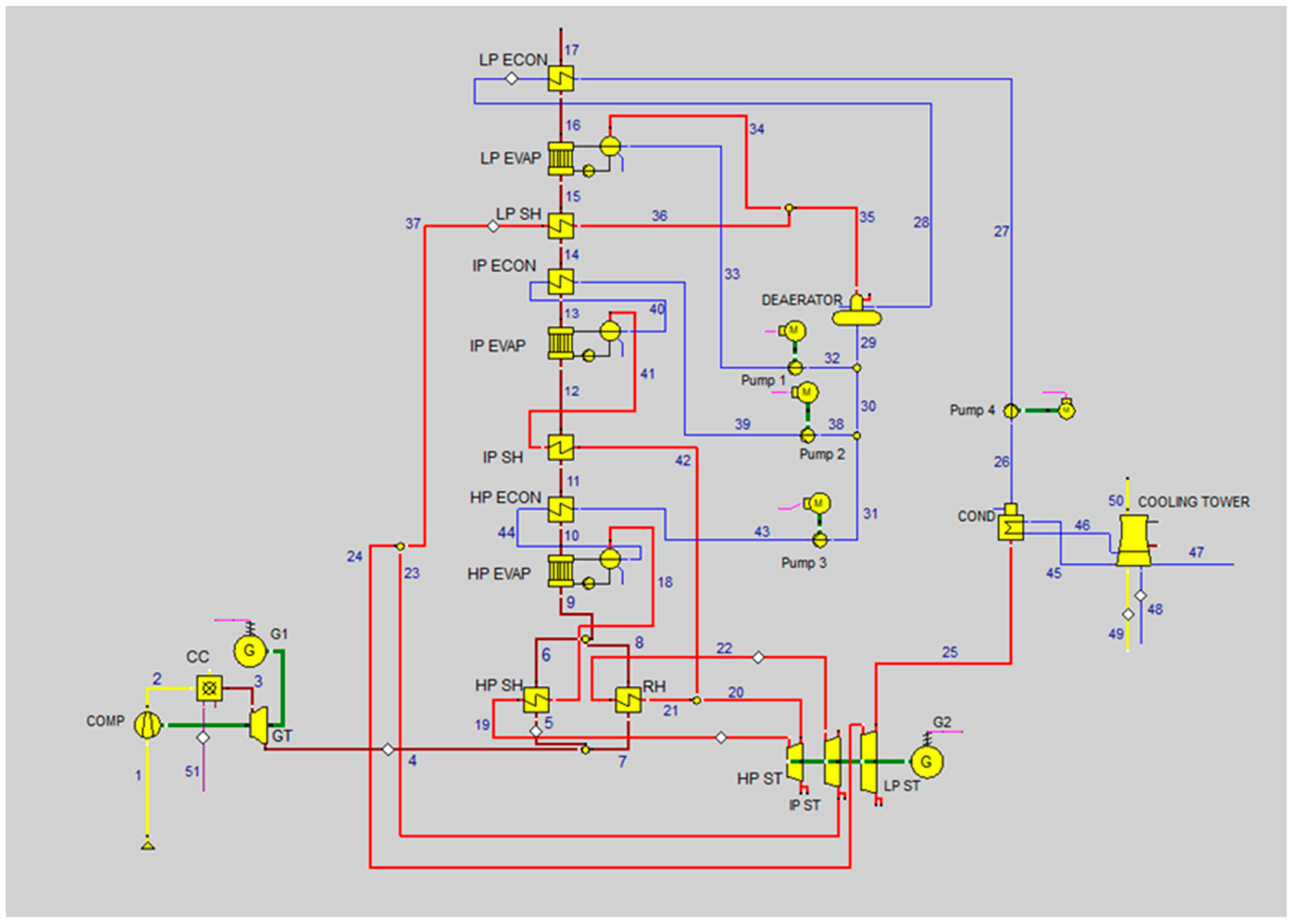
3.1. Simulation of the NGCC
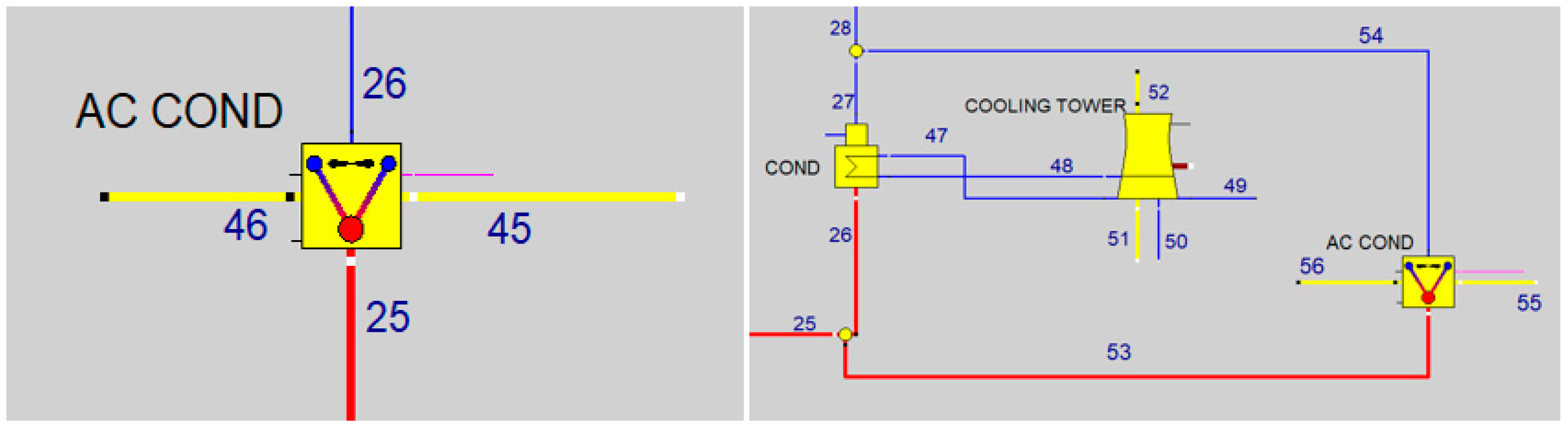
3.2. Simulation of the ISCC
4. Results
4.1. Exergetic Analysis
4.2. Economic Analysis
4.3. Exergoeconomic Analysis
5. Conclusions
Author Contributions
Funding
Acknowledgments
Conflicts of Interest
Nomenclature
| Abbreviations | |
| NGCC | natural gas combined-cycle |
| CSP | concentrated solar power |
| GT | gas turbine |
| ST | steam turbine |
| HRSG | heat recovery steam generator |
| HP | high pressure |
| ISCC | integrated solar combined-cycle |
| IP | intermediate pressure |
| LP | low pressure |
| SH | superheater |
| EVAP | evaporator |
| ECON | economizer |
| RH | reheater |
| COMP | compressor |
| CC | combustion chamber |
| G | generator |
| COND | condenser |
| AC COND | air-cooled condenser |
| DNI | direct normal irradiance |
| FCI | fixed capital investment |
| PEC | purchase equipment cost |
| O&M | operating and maintenance |
| TRR | total rate of return |
| COE | cost of electricity |
| Symbols | |
| exergy | |
| exergy rate | |
| cost per exergy unit | |
| cost rate of exergy stream/component | |
| temperature | |
| pressure | |
| mass flow rate | |
| ε | exergetic efficiency |
| exergy destruction ratio | |
| investment cost rate | |
| f | exergoeconomic factor |
| r | relative cost difference |
| Subscripts | |
| k | component index |
| D | destruction (exergy) |
| F | fuel (exergy) |
| P | product (exergy) |
| CH | chemical (exergy) |
| PH | physical (exergy) |
| TOT | total |
Appendix A

| Component | Exergy of the Fuel | Exergy of the Product | Exergy Destruction |
|---|---|---|---|
| Compressor | |||
| CC | |||
| GT | |||
| HPSH | |||
| RH | |||
| HPEvap | |||
| HPEcon | |||
| IPSH | |||
| IPEvap | |||
| IPEcon | |||
| LPSH | |||
| LPEvap | |||
| LPEcon | |||
| HPST | |||
| MPST | |||
| LPST | |||
| P1 | |||
| P2 | |||
| P3 | |||
| P4 | |||
| Cond | - | - | |
| Cooling Tower | - | - | |
| Deaerator | |||
| mixer 1 | |||
| mixer 2 | |||
| mixer 3 | |||
| Total |
| Component | Exergy of the Fuel | Exergy of the Product | Exergy Destruction |
|---|---|---|---|
| Compressor | |||
| CC | |||
| GT | |||
| HP2 SH | |||
| HP2 Evap | |||
| IP2 SH | |||
| HP2 Econ | |||
| IP2 Evap | |||
| IP2 Econ | |||
| LP2 Evap | |||
| LP2 Econ | |||
| Preheater | |||
| HP1 SH | |||
| HP1 Evap | |||
| HP1 Econ | |||
| IP1 SH | |||
| IP1 Evap | |||
| IP1 Econ | |||
| P1 | |||
| Solar field | |||
| ST1 | |||
| ST2 | |||
| ST3 | |||
| ST4 | |||
| P2 | |||
| P3 | |||
| P4 | |||
| P5 | |||
| Cond | - | - | |
| Cooling Tower | - | - | |
| Deaerator | |||
| mixer 1 | |||
| mixer 2 | |||
| mixer 3 | |||
| mixer 4 | |||
| mixer 5 | |||
| Total |
| Nr. | c (Cent/MJ) | (Cent/s) | (kg/s) | (°C) | p (bar) | |||
|---|---|---|---|---|---|---|---|---|
| 1 | 0.000 | 1.06 | 1.06 | 0.00 | 0.00 | 679.09 | 15.00 | 1.01 |
| 2 | 258.135 | 1.06 | 259.19 | 1.60 | 414.15 | 679.09 | 398.97 | 17.00 |
| 3 | 792.079 | 5.40 | 797.47 | 1.28 | 1017.96 | 693.75 | 1239.86 | 16.50 |
| 4 | 204.133 | 5.40 | 209.53 | 1.28 | 267.46 | 693.75 | 582.98 | 1.06 |
| 5 | 85.331 | 2.26 | 87.59 | 1.28 | 111.80 | 290.00 | 582.98 | 1.06 |
| 6 | 46.641 | 2.26 | 48.90 | 1.28 | 62.42 | 290.00 | 397.16 | 1.05 |
| 7 | 118.803 | 3.14 | 121.94 | 1.28 | 155.66 | 403.75 | 582.98 | 1.06 |
| 8 | 89.523 | 3.14 | 92.66 | 1.28 | 118.28 | 403.75 | 486.71 | 1.05 |
| 9 | 135.732 | 5.40 | 141.13 | 1.28 | 180.70 | 693.75 | 449.51 | 1.05 |
| 10 | 87.461 | 5.40 | 92.86 | 1.28 | 118.89 | 693.75 | 341.49 | 1.05 |
| 11 | 55.054 | 5.40 | 60.45 | 1.28 | 77.40 | 693.75 | 256.63 | 1.04 |
| 12 | 54.527 | 5.40 | 59.92 | 1.28 | 76.72 | 693.75 | 255.92 | 1.04 |
| 13 | 47.798 | 5.40 | 53.19 | 1.28 | 68.11 | 693.75 | 236.74 | 1.03 |
| 14 | 46.321 | 5.40 | 51.72 | 1.28 | 66.22 | 693.75 | 233.07 | 1.03 |
| 15 | 44.736 | 5.40 | 50.13 | 1.28 | 64.19 | 693.75 | 229.04 | 1.02 |
| 16 | 25.269 | 5.40 | 30.66 | 1.28 | 39.26 | 693.75 | 162.21 | 1.02 |
| 17 | 11.878 | 5.40 | 17.27 | 1.28 | 22.12 | 693.75 | 100.15 | 1.01 |
| 18 | 80.543 | 0.18 | 80.73 | 1.62 | 131.14 | 73.31 | 330.98 | 130.21 |
| 19 | 116.512 | 0.18 | 116.69 | 1.61 | 187.74 | 73.31 | 562.98 | 125.00 |
| 20 | 82.373 | 0.18 | 82.56 | 1.61 | 132.82 | 73.31 | 322.63 | 25.00 |
| 21 | 90.404 | 0.20 | 90.61 | 1.64 | 148.76 | 81.15 | 314.77 | 25.00 |
| 22 | 117.165 | 0.20 | 117.37 | 1.61 | 189.10 | 81.15 | 562.98 | 25.00 |
| 23 | 76.987 | 0.20 | 77.19 | 1.61 | 124.37 | 81.15 | 330.82 | 5.00 |
| 24 | 95.461 | 0.26 | 95.72 | 1.68 | 160.97 | 103.59 | 305.20 | 5.00 |
| 25 | 13.574 | 0.26 | 13.83 | 1.68 | 23.26 | 103.59 | 32.87 | 0.05 |
| 26 | 0.221 | 0.26 | 0.48 | 1.68 | 0.81 | 103.59 | 32.87 | 0.05 |
| 27 | 0.262 | 0.26 | 0.52 | 1.94 | 1.01 | 103.59 | 32.89 | 4.00 |
| 28 | 9.019 | 0.26 | 9.28 | 2.24 | 20.74 | 103.59 | 138.00 | 3.80 |
| 29 | 9.597 | 0.26 | 9.86 | 2.31 | 22.79 | 104.37 | 141.77 | 3.80 |
| 30 | 7.462 | 0.20 | 7.66 | 2.31 | 17.72 | 81.15 | 141.77 | 3.80 |
| 31 | 6.741 | 0.18 | 6.92 | 2.31 | 16.01 | 73.31 | 141.77 | 3.80 |
| 32 | 2.135 | 0.06 | 2.19 | 2.31 | 5.07 | 23.21 | 141.77 | 3.80 |
| 33 | 2.138 | 0.06 | 2.20 | 2.37 | 5.20 | 23.21 | 141.79 | 5.05 |
| 34 | 18.242 | 0.06 | 18.30 | 1.92 | 35.20 | 23.21 | 152.21 | 5.05 |
| 35 | 0.612 | 0.00 | 0.61 | 1.92 | 1.18 | 0.78 | 152.21 | 5.05 |
| 36 | 17.630 | 0.06 | 17.69 | 1.92 | 34.02 | 22.44 | 152.21 | 5.05 |
| 37 | 18.712 | 0.06 | 18.77 | 1.95 | 36.60 | 22.44 | 213.07 | 5.00 |
| 38 | 0.720 | 0.02 | 0.74 | 2.31 | 1.71 | 7.83 | 141.77 | 3.80 |
| 39 | 0.740 | 0.02 | 0.76 | 2.53 | 1.92 | 7.83 | 142.05 | 26.36 |
| 40 | 1.749 | 0.02 | 1.77 | 2.26 | 3.99 | 7.83 | 221.70 | 26.31 |
| 41 | 7.891 | 0.02 | 7.91 | 1.90 | 15.05 | 7.83 | 226.70 | 26.31 |
| 42 | 8.078 | 0.02 | 8.10 | 1.97 | 15.94 | 7.83 | 246.63 | 25.00 |
| 43 | 7.823 | 0.18 | 8.01 | 2.43 | 19.46 | 73.31 | 143.41 | 137.06 |
| 44 | 35.867 | 0.18 | 36.05 | 1.77 | 63.76 | 73.31 | 325.98 | 130.21 |
| 45 | 0.361 | 24.32 | 24.68 | 6.18 | 152.47 | 9736.49 | 17.26 | 1.01 |
| 46 | 4.307 | 24.32 | 28.63 | 6.18 | 176.85 | 9736.49 | 22.87 | 1.01 |
| 47 | 0.001 | 0.06 | 0.06 | 6.18 | 0.40 | 25.61 | 17.26 | 1.01 |
| 48 | 0.000 | 0.26 | 0.26 | 0.00 | 0.00 | 102.82 | 15.00 | 1.01 |
| 49 | 0.000 | 13.80 | 13.80 | 0.00 | 0.00 | 4868.20 | 15.00 | 1.01 |
| 50 | 1.061 | 7.15 | 8.21 | 3.20 | 26.29 | 4945.41 | 21.46 | 1.01 |
| 51 | 6.180 | 755.48 | 761.66 | 0.76 | 578.48 | 14.66 | 25.00 | 17.00 |
| Nr. | c (Cent/MJ) | (Cent/s) | (kg/s) | (°C) | (bar) | |||
|---|---|---|---|---|---|---|---|---|
| 1 | 0.000 | 1.07 | 1.07 | 0.00 | 0.00 | 690.55 | 15.00 | 1.01 |
| 2 | 262.489 | 1.07 | 263.56 | 1.59 | 418.28 | 690.55 | 398.97 | 17.00 |
| 3 | 805.440 | 5.49 | 810.93 | 1.27 | 1031.54 | 705.46 | 1239.86 | 16.50 |
| 4 | 207.577 | 5.49 | 213.06 | 1.27 | 271.03 | 705.46 | 582.98 | 1.06 |
| 5 | 85.331 | 2.26 | 87.59 | 1.27 | 111.41 | 290.00 | 582.98 | 1.06 |
| 6 | 46.045 | 2.26 | 48.30 | 1.27 | 61.44 | 290.00 | 393.95 | 1.05 |
| 7 | 122.246 | 3.23 | 125.48 | 1.27 | 159.61 | 415.46 | 582.98 | 1.06 |
| 8 | 92.458 | 3.23 | 95.69 | 1.27 | 121.72 | 415.46 | 487.86 | 1.05 |
| 9 | 138.022 | 5.49 | 143.51 | 1.28 | 183.16 | 705.46 | 449.51 | 1.05 |
| 10 | 88.936 | 5.49 | 94.42 | 1.28 | 120.51 | 705.46 | 341.49 | 1.05 |
| 11 | 55.982 | 5.49 | 61.47 | 1.28 | 78.45 | 705.46 | 256.63 | 1.04 |
| 12 | 55.446 | 5.49 | 60.93 | 1.28 | 77.77 | 705.46 | 255.92 | 1.04 |
| 13 | 48.605 | 5.49 | 54.09 | 1.28 | 69.04 | 705.46 | 236.74 | 1.03 |
| 14 | 47.102 | 5.49 | 52.59 | 1.28 | 67.12 | 705.46 | 233.07 | 1.03 |
| 15 | 45.491 | 5.49 | 50.98 | 1.28 | 65.06 | 705.46 | 229.04 | 1.02 |
| 16 | 25.695 | 5.49 | 31.18 | 1.28 | 39.80 | 705.46 | 162.21 | 1.02 |
| 17 | 12.079 | 5.49 | 17.56 | 1.28 | 22.42 | 705.46 | 100.15 | 1.01 |
| 18 | 81.902 | 0.19 | 82.09 | 1.62 | 132.77 | 74.55 | 330.98 | 130.21 |
| 19 | 118.477 | 0.19 | 118.66 | 1.60 | 189.86 | 74.55 | 562.98 | 125.00 |
| 20 | 83.762 | 0.19 | 83.95 | 1.60 | 134.32 | 74.55 | 322.63 | 25.00 |
| 21 | 91.929 | 0.21 | 92.13 | 1.63 | 150.44 | 82.52 | 314.77 | 25.00 |
| 22 | 119.141 | 0.21 | 119.35 | 1.60 | 191.49 | 82.52 | 562.98 | 25.00 |
| 23 | 78.286 | 0.21 | 78.49 | 1.60 | 125.94 | 82.52 | 330.82 | 5.00 |
| 24 | 97.071 | 0.26 | 97.33 | 1.67 | 162.96 | 105.33 | 305.20 | 5.00 |
| 25 | 13.802 | 0.26 | 14.07 | 1.67 | 23.55 | 105.33 | 32.87 | 0.05 |
| 26 | 0.224 | 0.26 | 0.49 | 1.67 | 0.82 | 105.33 | 32.87 | 0.05 |
| 27 | 0.266 | 0.26 | 0.53 | 1.93 | 1.02 | 105.33 | 32.89 | 4.00 |
| 28 | 9.171 | 0.26 | 9.43 | 2.23 | 21.00 | 105.33 | 138.00 | 3.80 |
| 29 | 9.758 | 0.27 | 10.02 | 2.30 | 23.05 | 106.13 | 141.77 | 3.80 |
| 30 | 7.588 | 0.21 | 7.79 | 2.30 | 17.92 | 82.52 | 141.77 | 3.80 |
| 31 | 6.855 | 0.19 | 7.04 | 2.30 | 16.19 | 74.55 | 141.77 | 3.80 |
| 32 | 2.171 | 0.06 | 2.23 | 2.30 | 5.13 | 23.61 | 141.77 | 3.80 |
| 33 | 2.174 | 0.06 | 2.23 | 2.35 | 5.25 | 23.61 | 141.79 | 5.05 |
| 34 | 18.549 | 0.06 | 18.61 | 1.91 | 35.61 | 23.61 | 152.21 | 5.05 |
| 35 | 0.622 | 0.00 | 0.62 | 1.91 | 1.19 | 0.79 | 152.21 | 5.05 |
| 36 | 17.928 | 0.06 | 17.98 | 1.91 | 34.42 | 22.81 | 152.21 | 5.05 |
| 37 | 19.027 | 0.06 | 19.08 | 1.94 | 37.02 | 22.81 | 213.07 | 5.00 |
| 38 | 0.733 | 0.02 | 0.75 | 2.30 | 1.73 | 7.97 | 141.77 | 3.80 |
| 39 | 0.753 | 0.02 | 0.77 | 2.51 | 1.94 | 7.97 | 142.05 | 26.36 |
| 40 | 1.779 | 0.02 | 1.80 | 2.24 | 4.04 | 7.97 | 221.70 | 26.31 |
| 41 | 8.025 | 0.02 | 8.04 | 1.89 | 15.22 | 7.97 | 226.70 | 26.31 |
| 42 | 8.215 | 0.02 | 8.23 | 1.96 | 16.12 | 7.97 | 246.63 | 25.00 |
| 43 | 7.955 | 0.19 | 8.14 | 2.42 | 19.67 | 74.55 | 143.41 | 137.06 |
| 44 | 36.472 | 0.19 | 36.66 | 1.76 | 64.53 | 74.55 | 325.98 | 130.21 |
| 45 | 0.000 | 85.80 | 85.80 | 0.00 | 0.00 | 30273.16 | 15.00 | 1.01 |
| 46 | 3.214 | 85.80 | 89.01 | 0.53 | 46.94 | 30273.16 | 22.87 | 1.01 |
| 47 | 6.284 | 768.23 | 774.51 | 0.76 | 588.24 | 14.91 | 25.00 | 17.00 |
| Nr. | c (Cent/MJ) | (Cent/s) | (kg/s) | (°C) | (bar) | |||
|---|---|---|---|---|---|---|---|---|
| 1 | 0.000 | 0.77 | 1.29 | 0.00 | 0.00 | 533.39 | 33.40 | 1.01 |
| 2 | 203.878 | 0.77 | 204.65 | 1.52 | 312.04 | 533.39 | 412.78 | 15.00 |
| 3 | 619.519 | 4.19 | 623.71 | 1.24 | 776.47 | 544.75 | 1231.88 | 14.50 |
| 4 | 171.565 | 4.19 | 175.76 | 1.24 | 218.80 | 544.75 | 604.99 | 1.03 |
| 5 | 103.974 | 4.19 | 108.17 | 1.24 | 134.66 | 544.75 | 439.19 | 1.02 |
| 6 | 69.503 | 4.19 | 73.70 | 1.24 | 91.75 | 544.75 | 340.68 | 1.02 |
| 7 | 67.692 | 4.19 | 71.88 | 1.24 | 89.49 | 544.75 | 335.35 | 1.02 |
| 8 | 52.306 | 4.19 | 56.50 | 1.24 | 70.34 | 544.75 | 285.61 | 1.02 |
| 9 | 45.039 | 4.19 | 49.23 | 1.24 | 61.29 | 544.75 | 260.06 | 1.02 |
| 10 | 35.797 | 4.19 | 39.99 | 1.24 | 49.78 | 544.75 | 225.39 | 1.02 |
| 11 | 21.034 | 4.19 | 25.23 | 1.24 | 31.41 | 544.75 | 159.84 | 1.02 |
| 12 | 20.390 | 4.19 | 24.58 | 1.24 | 30.60 | 544.75 | 157.01 | 1.02 |
| 13 | 5.482 | 4.19 | 9.67 | 1.24 | 12.04 | 544.75 | 46.10 | 1.01 |
| 14 | 344.442 | 3.88 | 344.44 | 0.96 | 330.35 | 1047.71 | 395.00 | 35.00 |
| 15 | 344.442 | 3.88 | 344.44 | 0.96 | 330.35 | 1047.71 | 395.00 | 35.00 |
| 16 | 329.205 | 3.88 | 329.20 | 0.96 | 315.74 | 1047.71 | 385.48 | 35.00 |
| 17 | 262.472 | 3.88 | 262.47 | 0.96 | 251.73 | 1047.71 | 340.83 | 35.00 |
| 18 | 226.053 | 3.88 | 226.05 | 0.96 | 216.80 | 1047.71 | 314.10 | 35.00 |
| 19 | 224.367 | 3.88 | 224.37 | 0.96 | 215.19 | 1047.71 | 312.82 | 34.99 |
| 20 | 204.434 | 3.88 | 204.43 | 0.96 | 196.07 | 1047.71 | 297.28 | 34.99 |
| 21 | 199.482 | 3.88 | 199.48 | 0.96 | 191.32 | 1047.71 | 293.32 | 34.99 |
| 22 | 201.636 | 3.88 | 201.64 | 0.98 | 197.85 | 1047.71 | 294.31 | 50.00 |
| 23 | 2.341 | 0.05 | 2.40 | 2.17 | 5.20 | 21.87 | 150.44 | 40.00 |
| 24 | 6.047 | 0.05 | 6.10 | 1.67 | 10.19 | 21.87 | 247.28 | 39.95 |
| 25 | 23.040 | 0.05 | 23.10 | 1.35 | 31.11 | 21.87 | 250.28 | 39.95 |
| 26 | 24.521 | 0.05 | 24.58 | 1.35 | 33.18 | 21.87 | 294.10 | 39.90 |
| 27 | 15.797 | 0.24 | 16.04 | 2.11 | 33.83 | 97.45 | 181.89 | 130.00 |
| 28 | 45.964 | 0.24 | 46.21 | 1.53 | 70.84 | 97.45 | 320.83 | 129.95 |
| 29 | 107.070 | 0.24 | 107.31 | 1.35 | 144.92 | 97.45 | 330.83 | 129.95 |
| 30 | 120.980 | 0.24 | 121.22 | 1.34 | 162.92 | 97.45 | 375.00 | 129.90 |
| 31 | 49.738 | 0.11 | 49.85 | 1.58 | 78.65 | 45.26 | 330.68 | 129.70 |
| 32 | 170.563 | 0.36 | 170.92 | 1.41 | 241.57 | 142.71 | 357.15 | 129.70 |
| 33 | 234.789 | 0.36 | 235.15 | 1.43 | 336.65 | 142.71 | 594.99 | 129.65 |
| 34 | 236.509 | 0.38 | 236.89 | 1.45 | 344.45 | 153.79 | 532.00 | 129.65 |
| 35 | 185.785 | 0.38 | 186.17 | 1.45 | 270.70 | 153.79 | 358.10 | 39.75 |
| 36 | 219.830 | 0.46 | 220.29 | 1.45 | 320.03 | 183.23 | 351.21 | 39.75 |
| 37 | 139.923 | 0.46 | 140.38 | 1.45 | 203.95 | 183.23 | 150.30 | 4.80 |
| 38 | 145.036 | 0.47 | 145.51 | 1.47 | 213.38 | 189.79 | 150.30 | 4.80 |
| 39 | 96.766 | 0.47 | 97.24 | 1.47 | 142.59 | 189.79 | 99.60 | 1.00 |
| 40 | 22.423 | 0.47 | 22.90 | 1.47 | 33.58 | 189.79 | 32.87 | 0.05 |
| 41 | 0.404 | 0.47 | 0.88 | 1.47 | 1.29 | 189.79 | 32.87 | 0.05 |
| 42 | 0.491 | 0.47 | 0.97 | 1.65 | 1.60 | 189.79 | 32.91 | 4.55 |
| 43 | 11.772 | 0.47 | 12.25 | 2.07 | 25.33 | 189.79 | 117.01 | 4.50 |
| 44 | 20.199 | 0.50 | 20.70 | 2.11 | 43.73 | 201.58 | 147.91 | 4.50 |
| 45 | 20.212 | 0.50 | 20.72 | 2.12 | 43.86 | 201.58 | 147.92 | 5.05 |
| 46 | 20.740 | 0.50 | 21.24 | 2.12 | 45.11 | 201.58 | 149.84 | 5.00 |
| 47 | 18.852 | 0.46 | 19.31 | 2.12 | 41.00 | 183.23 | 149.84 | 5.00 |
| 48 | 1.888 | 0.05 | 1.93 | 2.12 | 4.11 | 18.35 | 149.84 | 5.00 |
| 49 | 14.392 | 0.05 | 14.44 | 1.83 | 26.37 | 18.35 | 151.84 | 5.00 |
| 50 | 5.147 | 0.02 | 5.16 | 1.83 | 9.43 | 6.56 | 151.84 | 5.00 |
| 51 | 9.245 | 0.03 | 9.27 | 1.83 | 16.94 | 11.79 | 151.84 | 5.00 |
| 52 | - | - | - | - | - | 11.79 | 149.90 | 4.50 |
| 53 | 19.606 | 0.46 | 20.06 | 2.17 | 43.54 | 183.23 | 150.44 | 40.00 |
| 54 | 17.266 | 0.40 | 17.67 | 2.17 | 38.35 | 161.35 | 150.44 | 40.00 |
| 55 | 24.374 | 0.40 | 24.78 | 2.03 | 50.39 | 161.35 | 180.06 | 39.80 |
| 56 | 1.143 | 0.02 | 1.16 | 2.03 | 2.36 | 7.56 | 180.06 | 39.80 |
| 57 | 7.965 | 0.02 | 7.98 | 1.68 | 13.40 | 7.56 | 250.06 | 39.80 |
| 58 | 32.462 | 0.07 | 32.54 | 1.43 | 46.58 | 29.44 | 281.44 | 39.80 |
| 59 | 34.079 | 0.07 | 34.15 | 1.44 | 49.34 | 29.44 | 320.68 | 39.75 |
| 60 | 23.231 | 0.38 | 23.62 | 2.03 | 48.03 | 153.79 | 180.06 | 39.80 |
| 61 | 24.930 | 0.38 | 25.31 | 2.11 | 53.39 | 153.79 | 181.89 | 130.00 |
| 62 | 9.133 | 0.14 | 9.27 | 2.11 | 19.56 | 56.34 | 181.89 | 130.00 |
| 63 | 22.343 | 0.14 | 22.48 | 1.76 | 39.66 | 56.34 | 295.35 | 129.70 |
| 64 | 17.949 | 0.11 | 18.06 | 1.76 | 31.86 | 45.26 | 295.35 | 129.70 |
| 65 | 4.394 | 0.03 | 4.42 | 1.76 | 7.80 | 11.08 | 295.35 | 129.70 |
| 66 | 6.189 | 40.48 | 46.67 | 2.75 | 128.42 | 16207.28 | 22.31 | 1.01 |
| 67 | 18.858 | 40.48 | 59.34 | 2.75 | 163.28 | 16207.28 | 27.87 | 0.96 |
| 68 | 0.022 | 0.15 | 0.17 | 2.75 | 0.46 | 58.24 | 22.31 | 1.01 |
| 69 | 0.551 | 0.58 | 1.13 | 0.00 | 0.00 | 233.62 | 33.40 | 1.01 |
| 70 | 4.589 | 22.97 | 27.56 | 0.00 | 0.00 | 8103.56 | 33.40 | 1.01 |
| 71 | 6.476 | 12.02 | 18.49 | 2.01 | 37.14 | 8278.93 | 26.49 | 1.01 |
| 72 | 4.578 | 585.66 | 590.23 | 0.76 | 448.28 | 11.36 | 25.00 | 15.00 |
| Nr. | (MW) | (MW) | (MW) | c (Cent/MJ) | (Cent/s) | (kg/s) | (°C) | (bar) |
|---|---|---|---|---|---|---|---|---|
| 1 | 0.000 | 0.83 | 1.38 | 0.00 | 0.00 | 437.14 | 33.40 | 1.01 |
| 2 | 234.268 | 0.83 | 235.10 | 1.51 | 355.34 | 437.14 | 437.15 | 17.00 |
| 3 | 685.155 | 4.51 | 689.66 | 1.24 | 855.32 | 585.91 | 1251.70 | 16.50 |
| 4 | 179.669 | 4.51 | 184.18 | 1.24 | 228.42 | 585.91 | 594.64 | 1.03 |
| 5 | 112.354 | 4.51 | 116.86 | 1.24 | 144.93 | 585.91 | 440.50 | 1.02 |
| 6 | 74.754 | 4.51 | 79.26 | 1.24 | 98.30 | 585.91 | 340.68 | 1.02 |
| 7 | 72.818 | 4.51 | 77.33 | 1.24 | 95.90 | 585.91 | 335.39 | 1.02 |
| 8 | 56.706 | 4.51 | 61.21 | 1.24 | 75.92 | 585.91 | 287.04 | 1.02 |
| 9 | 48.442 | 4.51 | 52.95 | 1.24 | 65.67 | 585.91 | 260.06 | 1.02 |
| 10 | 38.969 | 4.51 | 43.48 | 1.24 | 53.92 | 585.91 | 227.12 | 1.02 |
| 11 | 22.623 | 4.51 | 27.13 | 1.24 | 33.65 | 585.91 | 159.84 | 1.02 |
| 12 | 21.957 | 4.51 | 26.47 | 1.24 | 32.82 | 585.91 | 157.13 | 1.02 |
| 13 | 7.791 | 4.51 | 12.30 | 1.24 | 15.25 | 585.91 | 67.07 | 1.01 |
| 14 | 344.442 | 3.88 | 344.44 | 0.95 | 326.08 | 1047.71 | 395.00 | 35.00 |
| 15 | 344.442 | 3.88 | 344.44 | 0.95 | 326.08 | 1047.71 | 395.00 | 35.00 |
| 16 | 329.205 | 3.88 | 329.20 | 0.95 | 311.66 | 1047.71 | 385.48 | 35.00 |
| 17 | 262.472 | 3.88 | 262.47 | 0.95 | 248.48 | 1047.71 | 340.83 | 35.00 |
| 18 | 226.053 | 3.88 | 226.05 | 0.95 | 214.00 | 1047.71 | 314.10 | 35.00 |
| 19 | 224.367 | 3.88 | 224.37 | 0.95 | 212.41 | 1047.71 | 312.82 | 34.99 |
| 20 | 204.434 | 3.88 | 204.43 | 0.95 | 193.54 | 1047.71 | 297.28 | 34.99 |
| 21 | 199.482 | 3.88 | 199.48 | 0.95 | 188.85 | 1047.71 | 293.32 | 34.99 |
| 22 | 201.636 | 3.88 | 201.64 | 0.97 | 195.27 | 1047.71 | 294.31 | 50.00 |
| 23 | 2.341 | 0.05 | 2.40 | 2.09 | 5.00 | 21.87 | 150.44 | 40.00 |
| 24 | 6.047 | 0.05 | 6.10 | 1.63 | 9.92 | 21.87 | 247.28 | 39.95 |
| 25 | 23.040 | 0.05 | 23.10 | 1.32 | 30.57 | 21.87 | 250.28 | 39.95 |
| 26 | 24.521 | 0.05 | 24.58 | 1.33 | 32.61 | 21.87 | 294.10 | 39.90 |
| 27 | 15.797 | 0.24 | 16.04 | 2.05 | 32.86 | 97.45 | 181.89 | 130.00 |
| 28 | 45.964 | 0.24 | 46.21 | 1.50 | 69.39 | 97.45 | 320.83 | 129.95 |
| 29 | 107.070 | 0.24 | 107.31 | 1.33 | 142.52 | 97.45 | 330.83 | 129.95 |
| 30 | 120.980 | 0.24 | 121.22 | 1.32 | 160.29 | 97.45 | 375.00 | 129.90 |
| 31 | 54.220 | 0.12 | 54.34 | 1.56 | 84.91 | 49.34 | 330.68 | 129.70 |
| 32 | 175.037 | 0.37 | 175.40 | 1.40 | 245.20 | 146.79 | 356.20 | 129.70 |
| 33 | 238.907 | 0.37 | 239.27 | 1.42 | 339.30 | 146.79 | 584.64 | 129.65 |
| 34 | 240.434 | 0.39 | 240.82 | 1.44 | 345.92 | 156.34 | 532.00 | 129.65 |
| 35 | 188.868 | 0.39 | 189.26 | 1.44 | 271.85 | 156.34 | 358.10 | 39.75 |
| 36 | 224.101 | 0.47 | 224.57 | 1.44 | 322.39 | 186.81 | 351.82 | 39.75 |
| 37 | 142.646 | 0.47 | 143.11 | 1.44 | 205.45 | 186.81 | 150.30 | 4.80 |
| 38 | 149.034 | 0.49 | 149.52 | 1.45 | 217.09 | 195.00 | 150.30 | 4.80 |
| 39 | 99.432 | 0.49 | 99.92 | 1.45 | 145.07 | 195.00 | 99.60 | 1.00 |
| 40 | 43.316 | 0.49 | 43.80 | 1.45 | 63.60 | 195.00 | 49.42 | 0.12 |
| 41 | 1.418 | 0.49 | 1.90 | 1.45 | 2.77 | 195.00 | 48.04 | 0.11 |
| 42 | 1.508 | 0.49 | 1.99 | 1.54 | 3.06 | 195.00 | 48.08 | 4.55 |
| 43 | 12.123 | 0.49 | 12.61 | 1.94 | 24.48 | 195.00 | 117.13 | 4.50 |
| 44 | 20.749 | 0.52 | 21.27 | 2.03 | 43.09 | 207.06 | 147.91 | 4.50 |
| 45 | 20.763 | 0.52 | 21.28 | 2.03 | 43.22 | 207.06 | 147.92 | 5.05 |
| 46 | 21.305 | 0.52 | 21.82 | 2.04 | 44.50 | 207.06 | 149.84 | 5.00 |
| 47 | 19.220 | 0.47 | 19.69 | 2.04 | 40.14 | 186.81 | 149.84 | 5.00 |
| 48 | 2.084 | 0.05 | 2.13 | 2.04 | 4.35 | 20.26 | 149.84 | 5.00 |
| 49 | 15.890 | 0.05 | 15.94 | 1.80 | 28.76 | 20.26 | 151.84 | 5.00 |
| 50 | 6.430 | 0.02 | 6.45 | 1.80 | 11.64 | 8.20 | 151.84 | 5.00 |
| 51 | 9.460 | 0.03 | 9.49 | 1.80 | 17.12 | 12.06 | 151.84 | 5.00 |
| 52 | - | - | - | - | - | 12.06 | 149.90 | 4.50 |
| 53 | 19.989 | 0.47 | 20.46 | 2.09 | 42.69 | 186.81 | 150.44 | 40.00 |
| 54 | 17.649 | 0.41 | 18.06 | 2.09 | 37.69 | 164.93 | 150.44 | 40.00 |
| 55 | 24.914 | 0.41 | 25.33 | 1.97 | 49.98 | 164.93 | 180.06 | 39.80 |
| 56 | 1.298 | 0.02 | 1.32 | 1.97 | 2.60 | 8.59 | 180.06 | 39.80 |
| 57 | 9.046 | 0.02 | 9.07 | 1.65 | 15.00 | 8.59 | 250.06 | 39.80 |
| 58 | 33.542 | 0.08 | 33.62 | 1.42 | 47.62 | 30.46 | 280.26 | 39.80 |
| 59 | 35.267 | 0.08 | 35.34 | 1.43 | 50.54 | 30.46 | 320.68 | 39.75 |
| 60 | 23.616 | 0.39 | 24.01 | 1.97 | 47.37 | 156.34 | 180.06 | 39.80 |
| 61 | 25.344 | 0.39 | 25.73 | 2.05 | 52.72 | 156.34 | 181.89 | 130.00 |
| 62 | 9.547 | 0.15 | 9.69 | 2.05 | 19.86 | 58.89 | 181.89 | 130.00 |
| 63 | 23.361 | 0.15 | 23.51 | 1.74 | 40.81 | 58.89 | 295.39 | 129.70 |
| 64 | 19.571 | 0.12 | 19.69 | 1.74 | 34.19 | 49.34 | 295.39 | 129.70 |
| 65 | 3.790 | 0.02 | 3.81 | 1.74 | 6.62 | 9.55 | 295.39 | 129.70 |
| 66 | 23.541 | 117.81 | 141.35 | 0.00 | 0.00 | 41567.60 | 33.40 | 1.01 |
| 67 | 53.564 | 117.81 | 171.37 | 0.57 | 98.52 | 41567.60 | 43.04 | 1.01 |
| 68 | 5.153 | 629.90 | 635.05 | 0.76 | 482.32 | 12.22 | 25.00 | 17.00 |
| Component | (MW) | (MW) | (%) | (%) | (%) | |||||||
|---|---|---|---|---|---|---|---|---|---|---|---|---|
| Compressor | 269.93 | 258.13 | 11.80 | 1.55 | 3.76 | 95.63 | 1.40 | 1.60 | 16.55 | 35.45 | 68.17 | 14.29 |
| CC | 761.66 | 538.28 | 223.38 | 29.29 | 71.15 | 70.67 | 0.76 | 1.12 | 169.66 | 25.32 | 12.99 | 47.37 |
| GT | 587.95 | 563.85 | 24.09 | 3.16 | 7.67 | 95.90 | 1.28 | 1.40 | 30.75 | 40.51 | 56.85 | 9.38 |
| HPSH | 38.69 | 35.97 | 2.72 | 0.36 | 0.87 | 93.03 | 1.28 | 1.57 | 3.47 | 7.20 | 67.48 | 22.66 |
| RH | 29.28 | 26.76 | 2.52 | 0.33 | 0.80 | 91.38 | 1.28 | 1.51 | 3.22 | 2.97 | 47.98 | 17.97 |
| HPEvap | 48.27 | 44.68 | 3.59 | 0.47 | 1.15 | 92.55 | 1.28 | 1.51 | 4.60 | 5.58 | 54.81 | 17.97 |
| HPEcon | 32.41 | 28.04 | 4.36 | 0.57 | 1.39 | 86.53 | 1.28 | 1.58 | 5.59 | 2.79 | 33.29 | 23.44 |
| IPSH | 0.53 | 0.19 | 0.34 | 0.04 | 0.11 | 35.48 | 1.28 | 4.78 | 0.44 | 0.22 | 33.33 | 273.44 |
| IPEvap | 6.73 | 6.14 | 0.59 | 0.08 | 0.19 | 91.29 | 1.28 | 1.80 | 0.75 | 2.44 | 76.49 | 40.63 |
| IPEcon | 1.48 | 1.01 | 0.47 | 0.06 | 0.15 | 68.31 | 1.28 | 2.05 | 0.60 | 0.18 | 23.08 | 60.16 |
| LPSH | 1.58 | 1.08 | 0.50 | 0.07 | 0.16 | 68.27 | 1.28 | 2.38 | 0.64 | 0.55 | 46.22 | 85.94 |
| LPEvap | 19.47 | 16.10 | 3.36 | 0.44 | 1.07 | 82.72 | 1.28 | 1.86 | 4.31 | 5.08 | 54.10 | 45.31 |
| LPEcon | 13.39 | 8.76 | 4.63 | 0.61 | 1.48 | 65.40 | 1.28 | 2.25 | 5.93 | 2.59 | 30.40 | 75.78 |
| HPST | 34.14 | 32.25 | 1.89 | 0.25 | 0.60 | 94.47 | 1.61 | 1.91 | 3.04 | 6.55 | 68.30 | 18.63 |
| MPST | 40.18 | 37.97 | 2.20 | 0.29 | 0.70 | 94.51 | 1.61 | 1.89 | 3.55 | 7.22 | 67.04 | 17.39 |
| LPST | 81.89 | 74.55 | 7.33 | 0.96 | 2.34 | 91.05 | 1.68 | 1.99 | 12.33 | 10.82 | 46.74 | 18.45 |
| P1 | 0.004 | 0.003 | 0.001 | 0.0001 | 0.0003 | 80.27 | 1.58 | 39.21 | 0.00 | 0.12 | 100.00 | 2381.65 |
| P2 | 0.02 | 0.02 | 0.005 | 0.001 | 0.002 | 80.28 | 1.58 | 10.63 | 0.01 | 0.17 | 94.44 | 572.78 |
| P3 | 1.35 | 1.08 | 0.27 | 0.03 | 0.08 | 80.29 | 1.58 | 3.19 | 0.42 | 1.32 | 75.86 | 101.90 |
| P4 | 0.05 | 0.04 | 0.01 | 0.002 | 0.00 | 78.35 | 1.58 | 4.92 | 0.02 | 0.12 | 85.71 | 211.39 |
| Cond | - | - | 9.41 | 1.23 | 3.00 | - | 22.46 | - | 211.24 | 1.92 | 0.90 | - |
| Cooling Tower | - | - | 9.72 | 1.27 | 3.10 | - | 24.38 | - | 237.02 | 2.32 | 0.97 | - |
| Deaerator | 0.54 | 0.51 | 0.03 | 0.004 | 0.01 | 93.77 | 1.92 | 3.77 | 0.06 | 0.87 | 93.55 | 96.35 |
| mixer 1 | 2.20 | 1.96 | 0.24 | 0.03 | 0.08 | 89.19 | 1.61 | 1.81 | 0.38 | - | - | 12.42 |
| mixer 2 | 0.70 | 0.65 | 0.05 | 0.01 | 0.02 | 93.18 | 1.61 | 1.73 | 0.08 | - | - | 7.45 |
| mixer 3 | 10.53 | 10.10 | 0.43 | 0.06 | 0.14 | 95.80 | 1.28 | 1.33 | 0.55 | - | - | 3.91 |
| TOTAL | 762.72 | 437.27 | 313.95 | 41.16 | 100.00 | 57.33 | 0.76 | 1.69 | 238.12 | 162.30 | - | - |
| Component | (MW) | (MW) | (MW) | (%) | (%) | (%) | (Cent/MJ) | (Cent/MJ) | (Cent/s) | (Cent/s) | (%) | (%) |
|---|---|---|---|---|---|---|---|---|---|---|---|---|
| Compressor | 274.49 | 262.49 | 12.00 | 1.55 | 3.78 | 95.63 | 1.40 | 1.59 | 16.75 | 35.02 | 67.65 | 13.57 |
| CC | 774.51 | 547.36 | 227.15 | 29.29 | 71.57 | 70.67 | 0.76 | 1.12 | 172.52 | 25.01 | 12.66 | 47.37 |
| GT | 597.86 | 573.37 | 24.50 | 3.16 | 7.72 | 95.90 | 1.27 | 1.40 | 31.16 | 40.02 | 56.22 | 10.24 |
| HPSH | 39.29 | 36.58 | 2.71 | 0.35 | 0.85 | 93.10 | 1.27 | 1.56 | 3.45 | 7.12 | 67.36 | 22.83 |
| RH | 29.79 | 27.21 | 2.58 | 0.33 | 0.81 | 91.35 | 1.27 | 1.51 | 3.28 | 3.16 | 49.07 | 18.90 |
| HPEvap | 49.09 | 45.43 | 3.66 | 0.47 | 1.15 | 92.55 | 1.28 | 1.50 | 4.67 | 5.59 | 54.48 | 17.19 |
| HPEcon | 32.95 | 28.52 | 4.44 | 0.57 | 1.40 | 86.53 | 1.28 | 1.57 | 5.66 | 2.80 | 33.10 | 22.66 |
| IPSH | 0.54 | 0.19 | 0.35 | 0.04 | 0.11 | 35.48 | 1.28 | 4.75 | 0.44 | 0.22 | 33.33 | 271.09 |
| IPEvap | 6.84 | 6.25 | 0.60 | 0.08 | 0.19 | 91.29 | 1.28 | 1.79 | 0.76 | 2.45 | 76.32 | 39.84 |
| IPEcon | 1.50 | 1.03 | 0.48 | 0.06 | 0.15 | 68.31 | 1.28 | 2.04 | 0.61 | 0.18 | 22.78 | 59.38 |
| LPSH | 1.61 | 1.10 | 0.51 | 0.07 | 0.16 | 68.27 | 1.28 | 2.37 | 0.65 | 0.55 | 45.83 | 85.16 |
| LPEvap | 19.80 | 16.38 | 3.42 | 0.44 | 1.08 | 82.72 | 1.28 | 1.85 | 4.37 | 5.09 | 53.81 | 44.53 |
| LPEcon | 13.62 | 8.90 | 4.71 | 0.61 | 1.48 | 65.40 | 1.28 | 2.24 | 6.01 | 2.59 | 30.12 | 75.00 |
| HPST | 34.71 | 32.80 | 1.92 | 0.25 | 0.60 | 94.47 | 1.60 | 1.89 | 3.07 | 6.47 | 67.82 | 18.13 |
| MPST | 40.86 | 38.61 | 2.24 | 0.29 | 0.71 | 94.51 | 1.60 | 1.88 | 3.60 | 7.13 | 66.45 | 17.50 |
| LPST | 83.27 | 75.81 | 7.46 | 0.96 | 2.35 | 91.05 | 1.67 | 1.98 | 12.48 | 10.69 | 46.14 | 18.56 |
| P1 | 0.004 | 0.003 | 0.001 | 0.0001 | 0.0003 | 80.26 | 1.57 | 38.58 | 0.00 | 0.12 | 100.00 | 2357.32 |
| P2 | 0.02 | 0.02 | 0.005 | 0.001 | 0.002 | 80.28 | 1.57 | 10.48 | 0.01 | 0.17 | 94.44 | 567.52 |
| P3 | 1.37 | 1.10 | 0.27 | 0.03 | 0.09 | 80.29 | 1.57 | 3.16 | 0.42 | 1.32 | 75.86 | 101.27 |
| P4 | 0.05 | 0.04 | 0.01 | 0.002 | 0.004 | 78.36 | 1.57 | 4.86 | 0.02 | 0.12 | 85.71 | 209.55 |
| AC cond | 107.06 | - | 17.57 | 2.26 | 5.53 | - | 0.32 | - | 5.59 | 12.86 | 69.70 | - |
| Deaerator | 0.55 | 0.51 | 0.03 | 0.004 | 0.01 | 93.77 | 1.91 | 3.71 | 0.07 | 0.86 | 92.47 | 94.24 |
| mixer 1 | 2.24 | 2.00 | 0.24 | 0.03 | 0.08 | 89.19 | 1.60 | 1.80 | 0.39 | - | - | 12.50 |
| mixer 2 | 0.71 | 0.66 | 0.05 | 0.01 | 0.02 | 93.18 | 1.60 | 1.72 | 0.08 | - | - | 7.50 |
| mixer 3 | 11.17 | 10.69 | 0.48 | 0.06 | 0.15 | 95.69 | 1.27 | 1.33 | 0.61 | - | - | 4.72 |
| TOTAL | 775.59 | 437.45 | 317.36 | 40.92 | 100.00 | 56.40 | 0.76 | 1.73 | 240.70 | 169.53 | - | - |
| Component | (MW) | (MW) | (MW) | (%) | (%) | (%) | (Cent/MJ) | (Cent/MJ) | (Cent/s) | (Cent/s) | (%) | (%) |
|---|---|---|---|---|---|---|---|---|---|---|---|---|
| Compressor | 212.46 | 203.36 | 9.09 | 1.54 | 5.85 | 95.72 | 1.36 | 1.53 | 12.39 | 22.61 | 64.60 | 12.50 |
| CC | 590.23 | 419.06 | 171.17 | 28.94 | 110.17 | 71.00 | 0.76 | 1.11 | 130.01 | 16.15 | 11.05 | 46.05 |
| GT | 447.95 | 428.33 | 19.62 | 3.32 | 12.63 | 95.62 | 1.24 | 1.36 | 24.43 | 25.84 | 51.40 | 9.68 |
| HP2 SH | 67.59 | 64.23 | 3.36 | 0.57 | 2.17 | 95.02 | 1.24 | 1.48 | 4.19 | 10.94 | 72.31 | 19.35 |
| HP2 Evap | 34.47 | 31.79 | 2.68 | 0.45 | 1.73 | 92.22 | 1.24 | 1.47 | 3.34 | 3.87 | 53.68 | 18.55 |
| IP2 SH | 1.81 | 1.62 | 0.19 | 0.03 | 0.13 | 89.24 | 1.24 | 1.70 | 0.24 | 0.50 | 67.57 | 37.10 |
| HP2 Econ | 15.39 | 13.21 | 2.18 | 0.37 | 1.40 | 85.85 | 1.24 | 1.52 | 2.71 | 0.95 | 25.96 | 22.58 |
| IP2 Evap | 7.27 | 6.82 | 0.44 | 0.08 | 0.29 | 93.89 | 1.24 | 1.62 | 0.55 | 1.99 | 78.35 | 30.65 |
| IP2 Econ | 9.24 | 7.11 | 2.13 | 0.36 | 1.37 | 76.90 | 1.24 | 1.69 | 2.66 | 0.54 | 16.88 | 36.29 |
| LP2 Evap | 14.76 | 12.50 | 2.26 | 0.38 | 1.45 | 84.70 | 1.24 | 1.78 | 2.81 | 3.89 | 58.06 | 43.55 |
| LP2 Econ | 0.64 | 0.53 | 0.12 | 0.02 | 0.08 | 81.88 | 1.24 | 2.37 | 0.15 | 0.45 | 75.00 | 91.13 |
| Preheater | 14.91 | 11.28 | 3.63 | 0.61 | 2.33 | 75.67 | 1.24 | 2.10 | 4.52 | 5.17 | 53.35 | 69.35 |
| HP1 SH | 15.24 | 13.91 | 1.33 | 0.22 | 0.85 | 91.29 | 0.96 | 1.29 | 1.27 | 3.39 | 72.75 | 34.38 |
| HP1 Evap | 66.73 | 61.11 | 5.63 | 0.95 | 3.62 | 91.57 | 0.96 | 1.21 | 5.40 | 10.08 | 65.12 | 26.04 |
| HP1 Econ | 36.42 | 30.17 | 6.25 | 1.06 | 4.02 | 82.83 | 0.96 | 1.23 | 6.00 | 2.08 | 25.74 | 28.13 |
| IP1 SH | 1.69 | 1.48 | 0.20 | 0.03 | 0.13 | 87.85 | 0.96 | 1.40 | 0.20 | 0.46 | 69.70 | 45.83 |
| IP1 Evap | 19.93 | 16.99 | 2.94 | 0.50 | 1.89 | 85.25 | 0.96 | 1.23 | 2.82 | 1.80 | 38.96 | 28.13 |
| IP1 Econ | 4.95 | 3.71 | 1.25 | 0.21 | 0.80 | 74.85 | 0.96 | 1.35 | 1.19 | 0.24 | 16.78 | 40.63 |
| P1 | 2.84 | 2.15 | 0.69 | 0.12 | 0.44 | 75.87 | 1.57 | 3.03 | 1.08 | 2.07 | 65.71 | 92.99 |
| Solar field | 263.99 | 142.81 | 121.18 | - | - | 54.10 | - | 0.93 | - | 132.50 | - | - |
| ST1 | 50.72 | 47.00 | 3.73 | 0.63 | 2.40 | 92.65 | 1.45 | 1.72 | 5.42 | 7.13 | 56.81 | 18.62 |
| ST2 | 79.91 | 72.02 | 7.88 | 1.33 | 5.07 | 90.14 | 1.45 | 1.74 | 11.45 | 9.22 | 44.61 | 20.00 |
| ST3 | 48.27 | 43.01 | 5.26 | 0.89 | 3.38 | 89.11 | 1.47 | 1.80 | 7.71 | 6.76 | 46.72 | 22.45 |
| ST4 | 74.34 | 64.89 | 9.45 | 1.60 | 6.08 | 87.29 | 1.47 | 1.81 | 13.85 | 8.60 | 38.31 | 23.13 |
| P2 | 0.02 | 0.01 | 0.005 | 0.001 | 0.003 | 73.36 | 1.57 | 9.82 | 0.01 | 0.10 | 90.91 | 525.48 |
| P3 | 1.03 | 0.75 | 0.27 | 0.05 | 0.18 | 73.43 | 1.57 | 3.37 | 0.43 | 0.93 | 68.38 | 114.65 |
| P4 | 2.29 | 1.70 | 0.59 | 0.10 | 0.38 | 74.23 | 1.57 | 3.15 | 0.93 | 1.76 | 65.43 | 100.64 |
| P5 | 0.13 | 0.09 | 0.04 | 0.01 | 0.03 | 68.99 | 1.57 | 3.54 | 0.06 | 0.11 | 64.71 | 125.48 |
| Cond | - | - | 9.35 | 1.58 | 6.02 | - | 32.29 | - | 301.89 | 2.57 | 0.84 | - |
| Cooling Tower | - | - | 22.70 | 3.84 | 14.61 | - | 34.86 | - | 791.16 | 2.74 | 0.35 | - |
| Deaerator | 8.06 | 7.25 | 0.82 | 0.14 | 0.53 | 89.86 | 1.83 | 2.23 | 1.49 | 1.46 | 49.49 | 21.86 |
| mixer 1 | 0.40 | 0.38 | 0.02 | 0.004 | 0.02 | 94.00 | 1.35 | 1.44 | 0.03 | - | - | 6.67 |
| mixer 2 | 4.51 | 4.36 | 0.15 | 0.03 | 0.10 | 96.58 | 1.34 | 1.39 | 0.21 | - | - | 3.73 |
| mixer 3 | 15.32 | 12.65 | 2.67 | 0.45 | 1.72 | 82.55 | 1.43 | 1.73 | 3.83 | - | - | 20.98 |
| mixer 4 | 1.27 | 1.24 | 0.03 | 0.01 | 0.02 | 97.36 | 1.45 | 1.49 | 0.05 | - | - | 2.76 |
| mixer 5 | 0.13 | 0.10 | 0.03 | 0.01 | 0.02 | 74.15 | 1.83 | 2.46 | 0.06 | - | - | 34.43 |
| TOTAL | 591.52 | 436.50 | 155.37 | 26.27 | 100.00 | 73.79 | 0.76 | 1.68 | 117.75 | 286.92 | - | - |
| Component | (MW) | (MW) | (MW) | (%) | (%) | (%) | (Cent/MJ) | (Cent/MJ) | (Cent/s) | (Cent/s) | (%) | (%) |
|---|---|---|---|---|---|---|---|---|---|---|---|---|
| Compressor | 243.80 | 233.72 | 10.09 | 1.58 | 6.42 | 95.86 | 1.36 | 1.52 | 13.68 | 24.73 | 64.38 | 11.76 |
| CC | 635.05 | 454.56 | 180.49 | 28.36 | 114.97 | 71.58 | 0.76 | 1.10 | 137.08 | 17.66 | 11.41 | 44.74 |
| GT | 505.49 | 483.14 | 22.35 | 3.51 | 14.24 | 95.58 | 1.24 | 1.36 | 27.72 | 28.26 | 50.48 | 9.68 |
| HP2 SH | 67.32 | 63.87 | 3.45 | 0.54 | 2.19 | 94.88 | 1.24 | 1.47 | 4.27 | 10.62 | 71.32 | 18.55 |
| HP2 Evap | 37.60 | 34.65 | 2.95 | 0.46 | 1.88 | 92.15 | 1.24 | 1.46 | 3.66 | 4.09 | 52.77 | 17.74 |
| IP2 SH | 1.94 | 1.73 | 0.21 | 0.03 | 0.13 | 89.12 | 1.24 | 1.69 | 0.26 | 0.52 | 66.67 | 36.29 |
| HP2 Econ | 16.11 | 13.81 | 2.30 | 0.36 | 1.46 | 85.74 | 1.24 | 1.52 | 2.85 | 0.97 | 25.39 | 22.58 |
| IP2 Evap | 8.26 | 7.75 | 0.52 | 0.08 | 0.33 | 93.76 | 1.24 | 1.60 | 0.64 | 2.15 | 77.06 | 29.03 |
| IP2 Econ | 9.47 | 7.27 | 2.21 | 0.35 | 1.41 | 76.70 | 1.24 | 1.69 | 2.74 | 0.54 | 16.46 | 36.29 |
| LP2 Evap | 16.35 | 13.81 | 2.54 | 0.40 | 1.62 | 84.46 | 1.24 | 1.77 | 3.15 | 4.13 | 56.73 | 42.74 |
| LP2 Econ | 0.67 | 0.54 | 0.12 | 0.02 | 0.08 | 81.32 | 1.24 | 2.36 | 0.15 | 0.45 | 75.00 | 90.32 |
| Preheater | 14.17 | 10.62 | 3.55 | 0.56 | 2.26 | 74.94 | 1.24 | 2.02 | 4.40 | 3.85 | 46.67 | 62.90 |
| HP1 SH | 15.24 | 13.91 | 1.33 | 0.21 | 0.85 | 91.29 | 0.95 | 1.28 | 1.26 | 3.34 | 72.61 | 34.74 |
| HP1 Evap | 66.73 | 61.11 | 5.63 | 0.88 | 3.58 | 91.57 | 0.95 | 1.20 | 5.33 | 9.96 | 65.14 | 26.32 |
| HP1 Econ | 36.42 | 30.17 | 6.25 | 0.98 | 3.98 | 82.83 | 0.95 | 1.21 | 5.92 | 2.05 | 25.72 | 27.37 |
| IP1 SH | 1.69 | 1.48 | 0.20 | 0.03 | 0.13 | 87.85 | 0.95 | 1.38 | 0.19 | 0.45 | 70.31 | 45.26 |
| IP1 Evap | 19.93 | 16.99 | 2.94 | 0.46 | 1.87 | 85.25 | 0.95 | 1.22 | 2.78 | 1.78 | 39.04 | 28.42 |
| IP1 Econ | 4.95 | 3.71 | 1.25 | 0.20 | 0.79 | 74.85 | 0.95 | 1.33 | 1.18 | 0.23 | 16.31 | 40.00 |
| P1 | 2.84 | 2.15 | 0.69 | 0.11 | 0.44 | 75.87 | 1.54 | 2.98 | 1.06 | 2.05 | 65.92 | 93.51 |
| Solar field | 263.99 | 142.81 | 121.18 | - | - | 54.10 | - | 0.92 | - | 130.81 | - | - |
| ST1 | 51.57 | 47.78 | 3.79 | 0.60 | 2.41 | 92.65 | 1.44 | 1.70 | 5.44 | 7.11 | 56.65 | 18.06 |
| ST2 | 81.45 | 73.42 | 8.03 | 1.26 | 5.12 | 90.14 | 1.44 | 1.72 | 11.53 | 9.20 | 44.38 | 19.44 |
| ST3 | 49.60 | 44.20 | 5.40 | 0.85 | 3.44 | 89.11 | 1.45 | 1.78 | 7.84 | 6.79 | 46.41 | 22.76 |
| ST4 | 56.12 | 49.27 | 6.84 | 1.08 | 4.36 | 87.80 | 1.45 | 1.80 | 9.94 | 7.20 | 42.01 | 24.14 |
| P2 | 0.02 | 0.01 | 0.005 | 0.001 | 0.003 | 73.36 | 1.54 | 9.58 | 0.01 | 0.10 | 90.91 | 522.08 |
| P3 | 1.05 | 0.77 | 0.28 | 0.04 | 0.18 | 73.43 | 1.54 | 3.31 | 0.43 | 0.93 | 68.38 | 114.94 |
| P4 | 2.33 | 1.73 | 0.60 | 0.09 | 0.38 | 74.23 | 1.54 | 3.09 | 0.92 | 1.76 | 65.67 | 100.65 |
| P5 | 0.13 | 0.09 | 0.04 | 0.01 | 0.02 | 69.75 | 1.54 | 3.32 | 0.06 | 0.10 | 62.50 | 115.58 |
| AC Cond | 52.42 | - | 22.40 | 3.52 | 14.27 | 1.91 | 1.47 | - | 32.91 | 21.48 | 39.49 | - |
| Deaerator | 8.25 | 7.42 | 0.83 | 0.13 | 0.53 | 89.89 | 1.80 | 2.21 | 1.50 | 1.49 | 49.83 | 22.78 |
| mixer 1 | 0.44 | 0.41 | 0.03 | 0.004 | 0.02 | 94.13 | 1.33 | 1.41 | 0.03 | - | - | 6.02 |
| mixer 2 | 4.78 | 4.62 | 0.16 | 0.03 | 0.10 | 96.61 | 1.32 | 1.37 | 0.21 | - | - | 3.79 |
| mixer 3 | 13.17 | 10.90 | 2.26 | 0.36 | 1.44 | 82.81 | 1.42 | 1.71 | 3.21 | - | - | 20.42 |
| mixer 4 | 1.31 | 1.28 | 0.03 | 0.01 | 0.02 | 97.36 | 1.44 | 1.48 | 0.05 | - | - | 2.78 |
| mixer 5 | 0.16 | 0.12 | 0.04 | 0.01 | 0.03 | 74.11 | 1.80 | 2.43 | 0.08 | - | - | 35.00 |
| TOTAL | 636.44 | 437.12 | 156.99 | 24.67 | 100.00 | 68.68 | 0.76 | 1.80 | 118.97 | 304.82 | - | - |
References
- Semertzidis, T.; Spataru, C.; Bleischwitz, R. Cross-sectional integration of the water-energy nexus in Brazil. J Sustain Dev Energy. J. Sustain. Dev. Energy Water Environ. Syst. 2018, 6, 114–128. [Google Scholar] [CrossRef]
- Lin, L.; Chen, Y. Evaluation of Future Water Use for Electricity Generation under Different Energy Development Scenarios in China. Sustainability 2017, 10, 30. [Google Scholar] [CrossRef]
- Rijsberman, F.R. Water scarcity: Fact or fiction? Agric. Water Manag. 2006, 80, 5–22. [Google Scholar] [CrossRef]
- Bieber, N.; Ker, J.H.; Wang, X.; Triantafyllidis, C.; van Dam, K.H.; Koppelaar, R.H.; Shah, N. Sustainable planning of the energy-water-food nexus using decision making tools. Energy Policy 2018, 113, 584–607. [Google Scholar] [CrossRef]
- Collins, R.; Kristensen, P.; Thyssen, N. Water Resources Across Europe—Confronting Water Scarcity and Drought; European Environment Agency: Copenhagen, Denmark, 2009. [CrossRef]
- Ali, B.; Kumar, A. Development of life cycle water-demand coefficients for coal-based power generation technologies. Energy Convers. Manag. 2015, 90, 247–260. [Google Scholar] [CrossRef]
- Förster, H.; Lilliestam, J. Modeling thermoelectric power generation in view of climate change. Reg. Environ. Chang. 2010, 10, 327–338. [Google Scholar] [CrossRef]
- Dodder, R.S. A review of water use in the U.S. electric power sector: Insights from systems-level perspectives. Curr. Opin. Chem. Eng. 2014, 5, 7–14. [Google Scholar] [CrossRef]
- Scanlon, B.R.; Duncan, I.; Reedy, R.C. Drought and the water-energy nexus in Texas. Environ. Res. Lett. 2013, 8. [Google Scholar] [CrossRef]
- Hadian, S.; Madani, K. The Water Demand of Energy: Implications for Sustainable Energy Policy Development. Sustainability 2013, 5, 4674–4687. [Google Scholar] [CrossRef]
- Miara, A. Thermal effluent from the power sector: An analysis of once-through cooling system impacts on surface water temperature. Environ. Res. Lett. 2013. [Google Scholar] [CrossRef]
- Zhai, H.; Rubin, E.S. Performance and cost of wet and dry cooling systems for pulverized coal power plants with and without carbon capture and storage. Energy Policy 2010, 38, 5653–5660. [Google Scholar] [CrossRef]
- Thopil, G.A.; Pouris, A. A 20 year forecast of water usage in electricity generation for South Africa amidst water scarce conditions. Renew. Sustain. Energy Rev. 2016, 62, 1106–1121. [Google Scholar] [CrossRef]
- Rezaei, E.; Shafiei, S.; Abdollahnezhad, A. Reducing water consumption of an industrial plant cooling unit using hybrid cooling tower. Energy Convers. Manag. 2010, 51, 311–319. [Google Scholar] [CrossRef]
- Alqahtani, B.J.; Patino-Echeverri, D. Integrated Solar Combined Cycle Power Plants: Paving the way for thermal solar. Appl. Energy 2016, 169, 1–23. [Google Scholar] [CrossRef]
- Frías, P.; Becerro González, F.J.; Junquera Delgado, A. Integración de plantas termosolares en ciclos combinados. Hibridación de fuentes renovables y fósiles en la generación eléctrica. Anales de Mecánica y Electricidad. 2013, XC, 27–32. [Google Scholar]
- Adem, U. A case study of PV-wind-diesel-battery hybrid system. J. Energy Syst. 2017, 1, 138–147. [Google Scholar] [CrossRef]
- Williams, C.R.; Rasul, M.G. Feasibility of a hybrid cooling system in a thermal power plant. In Proceedings of the 3rd IASME/WSEAS international conference on Energy & environment, Cambridge, UK, 23–25 February 2008; pp. 124–129. [Google Scholar]
- Achour, L.; Bouharkat, M.; Behar, O. Performance assessment of an integrated solar combined cycle in the southern of Algeria. Energy Rep. 2018, 4, 207–217. [Google Scholar] [CrossRef]
- Binamer, A.O. Al-Abdaliya integrated solar combined cycle power plant: Case study of Kuwait, part, I. Renew. Energy 2019, 131, 923–937. [Google Scholar] [CrossRef]
- Calise, F.; d’Accadia, M.D.; Libertini, L.; Vicidomini, M. Thermoeconomic analysis of an integrated solar combined cycle power plant. Energy Convers. Manag. 2018, 171, 1038–1051. [Google Scholar] [CrossRef]
- Bonforte, G.; Buchgeister, J.; Manfrida, G.; Petela, K. Exergoeconomic and exergoenvironmental analysis of an integrated solar gas turbine/combined cycle power plant. Energy 2018, 156, 352–359. [Google Scholar] [CrossRef]
- Ameri, M.; Mohammadzadeh, M. Thermodynamic, thermoeconomic and life cycle assessment of a novel integrated solar combined cycle (ISCC) power plant. Sustain. Energy Technol. Assess. 2018, 27, 192–205. [Google Scholar] [CrossRef]
- Scanlon, B.R.; Duncan, I.; Reedy, R.C.; Venkatesh, A.; Jaramillo, P.; Griffin, W.M. Marginal costs of water savings from cooling system retrofits: A case study for Texas power plants 2008, Environmental Research Letters. Available online: https://iopscience.iop.org/article/10.1088/1748-9326/11/10/104004/meta (accessed on 7 April 2019).
- Reddy, V.S.; Kaushik, S.C.; Tyagi, S.K.; Panwar, N. An Approach to Analyse Energy and Exergy Analysis of Thermal Power Plants: A Review. Smart Grid Renew. Energy 2010, 1, 143–152. [Google Scholar] [CrossRef]
- Petrakopoulou, F.; Tsatsaronis, G.; Morosuk, T.; Carassai, A. Conventional and advanced exergetic analyses applied to a combined cycle power plant. Energy 2012, 41, 146–152. [Google Scholar] [CrossRef]
- Kaushik, S.C.; Reddy, V.S.; Tyagi, S.K. Energy and exergy analyses of thermal power plants: A review. Renew. Sustain. Energy Rev. 2011, 15, 1857–1872. [Google Scholar] [CrossRef]
- Kotas, T.J. Introduction. Exergy Method Therm. Plant Anal. 1985. [Google Scholar] [CrossRef]
- Zhao, Y.; Wang, S.; Ge, M.; Li, Y.; Yang, Y. Energy and exergy analysis of thermoelectric generator system with humidified flue gas. Energy Convers. Manag. 2018, 156, 140–149. [Google Scholar] [CrossRef]
- Verma, Y.; Kaurase, K.P. Exergy Analysis of Thermal Power Plant: A Review. N. Eng. J. Med. 2013, 2, 668–673. [Google Scholar] [CrossRef]
- Koroneos, C.; Polyzakis, A.; Xydis, G.; Stylos, N.; Nanaki, E. Exergy analysis for a proposed binary geothermal power plant in Nisyros Island, Greece. Geothermics 2017, 70, 38–46. [Google Scholar] [CrossRef]
- Sahoo, U.; Kumar, R.; Singh, S.K.; Tripathi, A.K. Energy, exergy, economic analysis and optimization of polygeneration hybrid solar-biomass system. Appl. Therm. Eng. 2018, 145, 685–692. [Google Scholar] [CrossRef]
- Wang, L.; Yang, Y.; Dong, C.; Yang, Z.; Xu, G.; Wu, L. Exergoeconomic evaluation of a modern ultra-supercritical power plant. Energies 2012, 5, 3381–3397. [Google Scholar] [CrossRef]
- Bejan, A.; Tsatsaronis, G.; Moran, M. Thermal Design and Optimization; Wiley-Interscience: New York, NY, USA, 1996. [Google Scholar]
- Petrakopoulou, F. Comparative Evaluation of Power Plants with CO2 Capture: Thermodynamic, Economic and Environmental Performance; Institut für Energietechnik: Amberg, Germany, 2010. [Google Scholar]


| Ambient Air |
| 15 °C, 1.013 bar, 60% relative humidity |
| Composition (mol %): N2 (75.04), O2 (22.99), CO2 (0.05), H2O (0.63), Ar (1.28) |
| Fuel |
| 14.66 kg/s (wet cooling)/14.91 kg/s (dry cooling), 25 °C, 17 bar, LHV = 50,015 kJ/kg |
| Natural gas composition (mol %): CH4 (100.0) |
| Gas Turbine System |
| Compressor: isentropic efficiency, 90.0%; mechanical efficiency, 99%; pressure ratio, 16.8 |
| Gas turbine: isentropic efficiency: 91%; mechanical efficiency: 99% |
| Generators: electrical efficiency, 98.5% |
| Steam Cycle Overall Plants |
| HRSG: 1 reheat stage, 3 pressure levels: HP (125 bar), IP (25 bar), LP (5 bar) |
| HRSG pressure drop: hot side, 5 mbar; cold side, 5% |
| SHs: ∆Tmin, 20 °C (HP, LP); ∆Tmin: 10 °C (IP) |
| EVAPs (HP, IP): approach temperature, 5 °C; pinch point: 10 °C |
| EVAP (LP): approach temperature, given externally; pinch point: 10 °C |
| Live steam temperature: 563 °C |
| Steam turbine isentropic efficiency (HP, IP, LP): 92% |
| Steam turbine mechanical efficiency (HP, IP, LP): 99% |
| Pumps efficiencies: 85%–87.2% (incl. motors and mechanical efficiency: 98%–99.8%) |
| Wet Cooling System |
| Condenser operating pressure: 0.05 bar |
| Cooling water temperature: 17.27 °C |
| Make-up water mass flow: 102.84 kg/s |
| Dry Cooling System |
| Air-cooled condenser operating pressure: 0.05 bar |
| Cooling air temperature: 1 °C |
| Power input to work the fan: 7.2 MW |
| Ambient Air |
| 33.4 °C, 1.013 bar, 60% relative humidity |
| Composition (mol %): N2 (74.07), O2 (22.69), CO2 (0.04), H2O (1.93), Ar (1.27) |
| Fuel |
| 11.37 kg/s (wet cooling)/12.22 kg/s (dry cooling), 25 °C, 15 bar, LHV = 50,015 kJ/kg |
| Natural gas composition (mol %): CH4 (100.0) |
| Gas Turbine System |
| Compressor: isentropic efficiency, 90.0%; mechanical efficiency, 99%; pressure ratio: 14.8 |
| Gas turbine: isentropic efficiency, 91%; mechanical efficiency, 99% |
| Generators: electrical efficiency, 98.5% |
| Steam Cycle Overall Plants |
| HRSG, 3 pressure levels: HP (129.65 bar), IP (39.75 bar), LP (4.8 bar) |
| HRSG pressure drop: |
| - SHs, ECON (LP), Preheater: hot side, 0.05 bar; cold side, 2 mbar |
| - EVAPs: hot side, 0.002 bar; cold side: 0 bar |
| - ECON (HP): hot side, 0.3 bar; cold side: 0.002 bar |
| - ECON (IP): hot side, 0.2 bar; cold side: 0 mbar |
| SHs: ∆Tmin, 10 °C (HP); ∆Tmin: 20 °C (IP) |
| ECONs: ∆Tmin, 40 °C (HP); ∆Tmin, 80 °C (IP); ∆Tmin, 10 °C (LP) |
| Preheater: ∆Tmin, 40 °C |
| EVAPs (HP, IP, LP): approach temperature, given externally; pinch point, 10 °C |
| Live steam temperature: 532 °C |
| Steam turbine isentropic efficiency (ST1, ST2, ST3, ST4): 88% |
| Steam turbine mechanical efficiency (ST1, ST2, ST3, ST4): 99% |
| Pumps efficiencies: 85% (incl. motors and mechanical efficiency: 99.8%) |
| Solar Field and HRSG 1 |
| Solar field |
| Sun DNI: 950 W/m2 |
| Number of collectors: 7500 |
| Collector length: 10 m |
| Gross aperture width: 5.76 m |
| Focal length: 1.71 m |
| Pressure loss: 15 bar |
| HRSG, 2 pressure levels: HP (129.9 bar), IP (39.9 bar) |
| HRSG pressure drop: |
| SHs, ECONs (HP, IP): hot side, 50 mbar; cold side: 0.002 bar |
| EVAPs: hot side, 0.002 bar; cold side: 0 bar |
| SHs: ∆Tmin, 20 °C (HP, IP) |
| ECONs: ∆Tmin, 20 °C (HP); ∆Tmin, 50 °C (IP) |
| EVAPs: (HP) approach temperature, given externally; pinch point, 10 °C (IP) approach temperature, given externally; pinch point, 47 °C |
| Wet Cooling System |
| Condenser operating pressure: 0.05 bar |
| Cooling water temperature: 22.31 °C |
| Supplemented water mass flow: 233.62 kg/s |
| Dry Cooling System |
| Air-cooled condenser operating pressure: 0.12 bar |
| Cooling air temperature: 33.4 °C (Tamb) |
| Power input to work the fan: 10.5 MW |
| Parameters | NGCC | ISCC | ||||
|---|---|---|---|---|---|---|
| Wet Cooling Simulation | Dry Cooling Simulation | Hybrid Cooling Simulation | Wet Cooling Simulation | Dry Cooling Simulation | Hybrid Cooling Simulation | |
| εtot (%) | 57.3 | 56.4 | 56.8 | 73.8 | 68.7 | 71.2 |
| (MW) | 762.7 | 775.6 | 769.2 | 591.5 | 636.4 | 614.0 |
| (MW) | 437.3 | 437.5 | 437.1 | 436.5 | 437.1 | 437.1 |
| (MW) | 314.0 | 317.4 | 316.1 | 155.4 | 157.0 | 156.2 |
| (%) | 41.2 | 40.9 | 41.1 | 26.3 | 24.7 | 25.4 |
| Dynamic Simulation Results | Wet Cooling Simulation | Dry Cooling Simulation | Hybrid Cooling Simulation |
|---|---|---|---|
| εtot (%) | 63.4 | 62.3 | 62.9 |
| (MW) | 689.0 | 701.1 | 695.0 |
| (MW) | 436.5 | 437.1 | 437.1 |
| Parameters | NGCC | ISCC | ||||
|---|---|---|---|---|---|---|
| Wet Cooling Simulation | Dry Cooling Simulation | Hybrid Cooling Simulation | Wet Cooling Simulation | Dry Cooling Simulation | Hybrid Cooling Simulation | |
| Total FCI (M€) | 204 | 214 | 218 | 385 | 411 | 417 |
| Cooling system FCI (M€) | 4.2 | 13.6 | 17.8 | 6.1 | 26.4 | 32.4 |
| Parameters | NGCC | ISCC | ||||
|---|---|---|---|---|---|---|
| Wet Cooling Simulation | Dry Cooling Simulation | Hybrid Cooling Simulation | Wet Cooling Simulation | Dry Cooling Simulation | Hybrid Cooling Simulation | |
| COE (cent/kWh) | 6.10 | 6.24 | 6.23 | 6.06 | 6.48 | 6.39 |
| (cent/s) | 579.7 | 589.4 | 584.5 | 449.5 | 483.7 | 466.6 |
| (cent/s) | 162.3 | 169.5 | 172.5 | 286.9 | 304.8 | 308.8 |
| NGCC | ISCC |
|---|---|
| Higher fuel consumption | Lower fuel consumption: higher efficiency |
| Continuous performance, independent from ambient conditions | Performance depends on the ambient conditions |
| Lower cooling system capacity | Solar field provides the ST with additional steam → Higher steam mass flow passing through the cooling system (higher cooling system capacity) |
| Lower investment cost | Much higher investment cost due to the addition of the solar field |
| Wet Cooling | Dry Cooling | Hybrid Cooling |
|---|---|---|
| Highest water consumption | Approximately zero water consumption | Half the water consumption of the wet cooling |
| Lowest investment cost | High investment cost | Highest investment cost: sum of the wet cooling and the dry cooling investment costs |
| Zero power input required in the cooling system | Power input required to work the air-cooled condenser fan | Requires power input: half of the power input required for the dry cooling |
| Lowest COE | Highest COE | COE in between that of the wet and dry cooling systems |
© 2019 by the authors. Licensee MDPI, Basel, Switzerland. This article is an open access article distributed under the terms and conditions of the Creative Commons Attribution (CC BY) license (http://creativecommons.org/licenses/by/4.0/).
Share and Cite
Petrakopoulou, F.; Olmeda-Delgado, M. Studying the Reduction of Water Use in Integrated Solar Combined-Cycle Plants. Sustainability 2019, 11, 2085. https://doi.org/10.3390/su11072085
Petrakopoulou F, Olmeda-Delgado M. Studying the Reduction of Water Use in Integrated Solar Combined-Cycle Plants. Sustainability. 2019; 11(7):2085. https://doi.org/10.3390/su11072085
Chicago/Turabian StylePetrakopoulou, Fontina, and Marina Olmeda-Delgado. 2019. "Studying the Reduction of Water Use in Integrated Solar Combined-Cycle Plants" Sustainability 11, no. 7: 2085. https://doi.org/10.3390/su11072085
APA StylePetrakopoulou, F., & Olmeda-Delgado, M. (2019). Studying the Reduction of Water Use in Integrated Solar Combined-Cycle Plants. Sustainability, 11(7), 2085. https://doi.org/10.3390/su11072085