Article

Optimization of Concrete Mixture Design Using Adaptive Surrogate Model

1
MOE Key Laboratory of Deep Earth Science and Engineering, College of Architecture and Environment, Sichuan University, Chengdu 610065, China
2
Failure Mechanics and Engineering Disaster Prevention and Mitigation Key Lab of Sichuan Province, Chengdu 610065, China
3
Department of Architectural Engineering, Kaili University, Kaili 556011, China
4
School of Mechanical Engineering, Chengdu University, Chengdu 610106, China
*
Authors to whom correspondence should be addressed.
Sustainability 2019, 11(7), 1991; https://doi.org/10.3390/su11071991
Submission received: 8 February 2019 / Revised: 20 March 2019 / Accepted: 21 March 2019 / Published: 3 April 2019

Abstract

:
The increase in urban construction in China has been accompanied by increasing concrete output, which has reached 2250 million m3 in recent years, ranked as the highest in the world. Consequentially, its environmental burden is significant in terms of resource use and carbon emissions. An adaptive surrogate model based on an extended radial basis function and adaptive sampling method was used to optimize the design of a concrete mixture in order to reduce its CO2 emissions and cost. The adaptive sampling method based on the multi-island genetic algorithm was adopted in order to improve the adaptive capability and accuracy of the surrogate model by selecting the proper sample size and ensuring uniform distribution of the sample points in the designed space. Three types of concrete with different strength, that is, C70, C40 and C30, were optimized by controlling the amount of fly ash and phosphorous slag in the samples. The optimized results showed that fly ash and phosphorous slag have a significant influence on the CO2 emissions of concrete and optimized concrete’s cost, while CO2 emissions were less than that of the reference samples. Therefore, the optimal mixture is with great significance to reduce the carbon emission of concrete, which also has implications for decreasing the environmental burden of concrete. In this way, we can optimize concrete of different strength to reduce carbon dioxide emission.

1. Introduction

The increase in urban construction in China has been accompanied by an increasing concrete output. Concrete output and year on year growth of China in the period 2006–2017 is shown in Figure 1. The left y axis represents the annual increase of China’s concrete production, which tended to be stable from 2013 to 2017 and had reached 2250 million m3, ranked as the highest in the world [1]. The right y axis reflects the slight change of year-over-year growth from 2014 to 2017, which indicated that concrete tends to be stable in these years. Ordinary Portland cement (OPC), a traditional cementitious material in concrete, requires large amounts of energy for production and the manufacture of 1 ton of cement releases 1 ton of CO2 [2,3]. Globally, 4.1 billion tons of Ordinary Portland cement were produced in 2015, which corresponds to 25–30 billion tons of concrete [4], accounting for 8–9% of the global man-made CO2 emissions [5]. Therefore, in order to reduce CO2 emissions from concrete, many researchers have concentrated on developing cementitious materials to replace OPC, such as fly ash, phosphorous slag and ground granulated blast furnace slag [6,7]. Meanwhile, many optimization design strategies have been designed to produce low-carbon-emission [8] and low-cost concrete [9,10].
Evolutionary algorithms and genetic algorithms (GAs) were the main traditional optimization methods for reducing CO2 emissions and cost of concrete [11,12]. However, recently, other optimization methods have been developed. For example, Camp and Assadollahi (2013) optimized the CO2 emissions and cost of reinforced concrete frames by using a big bang-big crunch algorithm [13]. Le et al. (2018) proposed simulated annealing (SA) to lower the CO2 emissions and cost of reinforced concrete frames [14]. Hong et al. (2012) built an integrated model to estimate the CO2 emissions and cost of ready-mixture concrete in order to realize sustainable structural design [15]. However, these studies indicated that the optimization methods depend on a lot of experimental data, which could consume a lot of computing time, equipment and materials so on [16]. The surrogate model was originally developed using optimum structural design [17] based on an approximate mathematical model, which can replace more complex and time-consuming numerical analysis in the analysis and optimization design process. The surrogate model cannot only improve the optimization design efficiency but also reduce the difficulty of optimization [18]. The techniques associated with the surrogate model include the response surface methodology (RSM), the kriging method, the radial basis function (RBF) and the extended radial basis function (ERBF) [19,20]. The ERBF method is the most flexible of these [21]. In addition, all the alternative model methods showed no indication of adaptation at the sampling point [22,23,24]. Thus, in this study, in order to optimize a concrete mixture to achieve the lowest CO2 emissions and cost, a surrogate model was built using the ERBF and the adaptive sampling method. The latter was adopted to enhance the adaptive capability and accuracy of the surrogate model by selecting the proper sample size and ensuring all the sample points are uniformly distributed in the design range [25].
However, the environmental burden of concrete is not limited to only CO2 emissions in one specific stage of the process. The analysis and quantification of the overall environmental impacts of concrete production require a holistic analytical approach [26]. The most suitable approach for this is life-cycle assessment (LCA), which is mainly used to estimate the environmental impact (e.g., global warming) of a product from cradle to grave. Peng and Pheng (2011) calculated the overall CO2 generated during the production cycle of precast concrete columns [27]. The cost over the life cycle can also be calculated based on the LCA; for example, Mclellan et al. (2011) compared the lifecycle cost and CO2 emissions of OPC and geopolymers in Australia [9]. The objective of this paper is to optimize concrete mixture design using adaptive surrogate model in order to mitigate its CO2 emissions and cost.

2. Materials and Methods

The design of the concrete mixture optimization process was divided into four steps: (i) selecting sample points using LHS; (ii) building an adaptive surrogate model of concrete mixtures with three different strengths; (iii) calculating the cost and CO2 emissions of concrete; and (iv) combining the GA with the model to select the optimal concrete mixture.

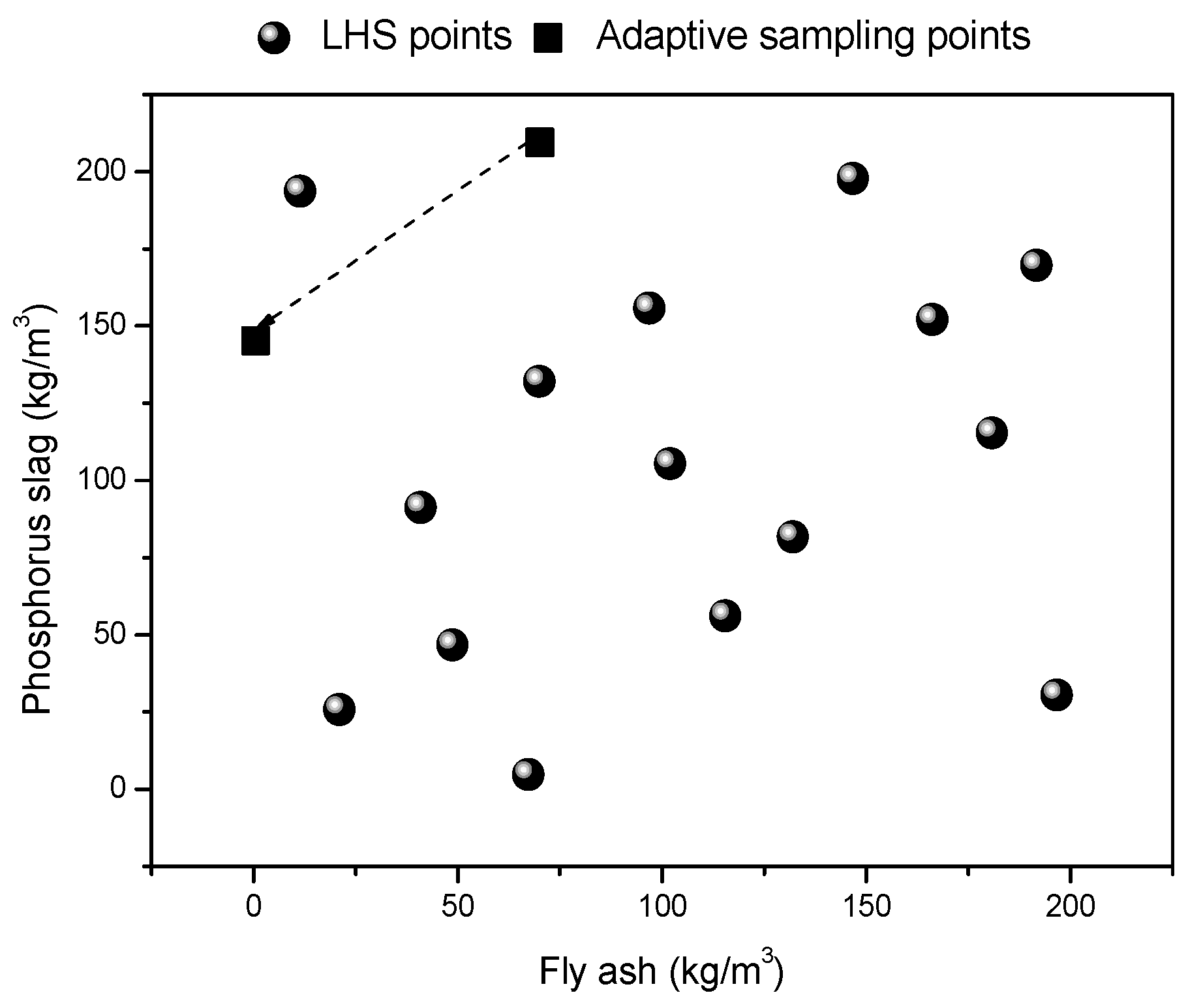
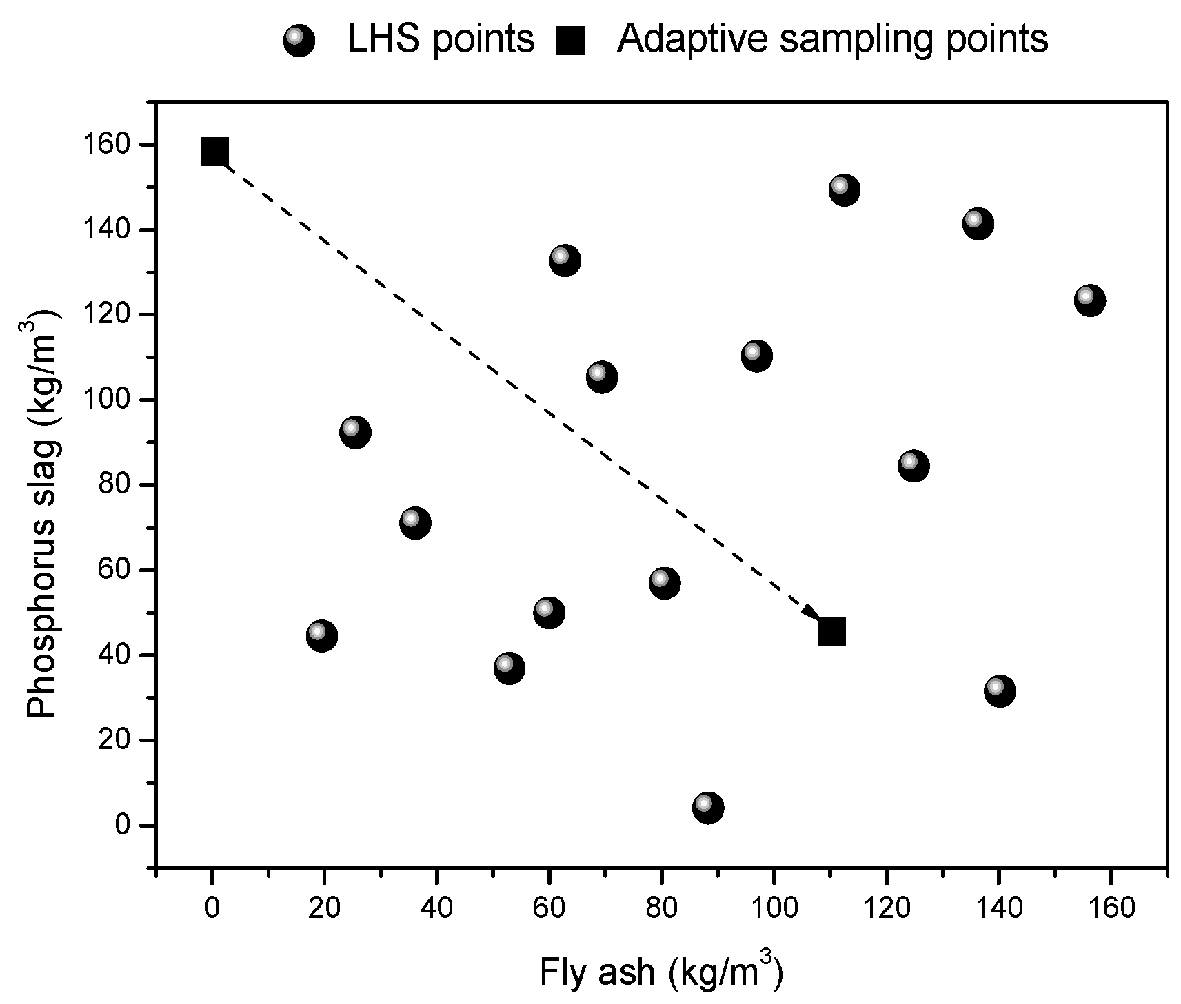
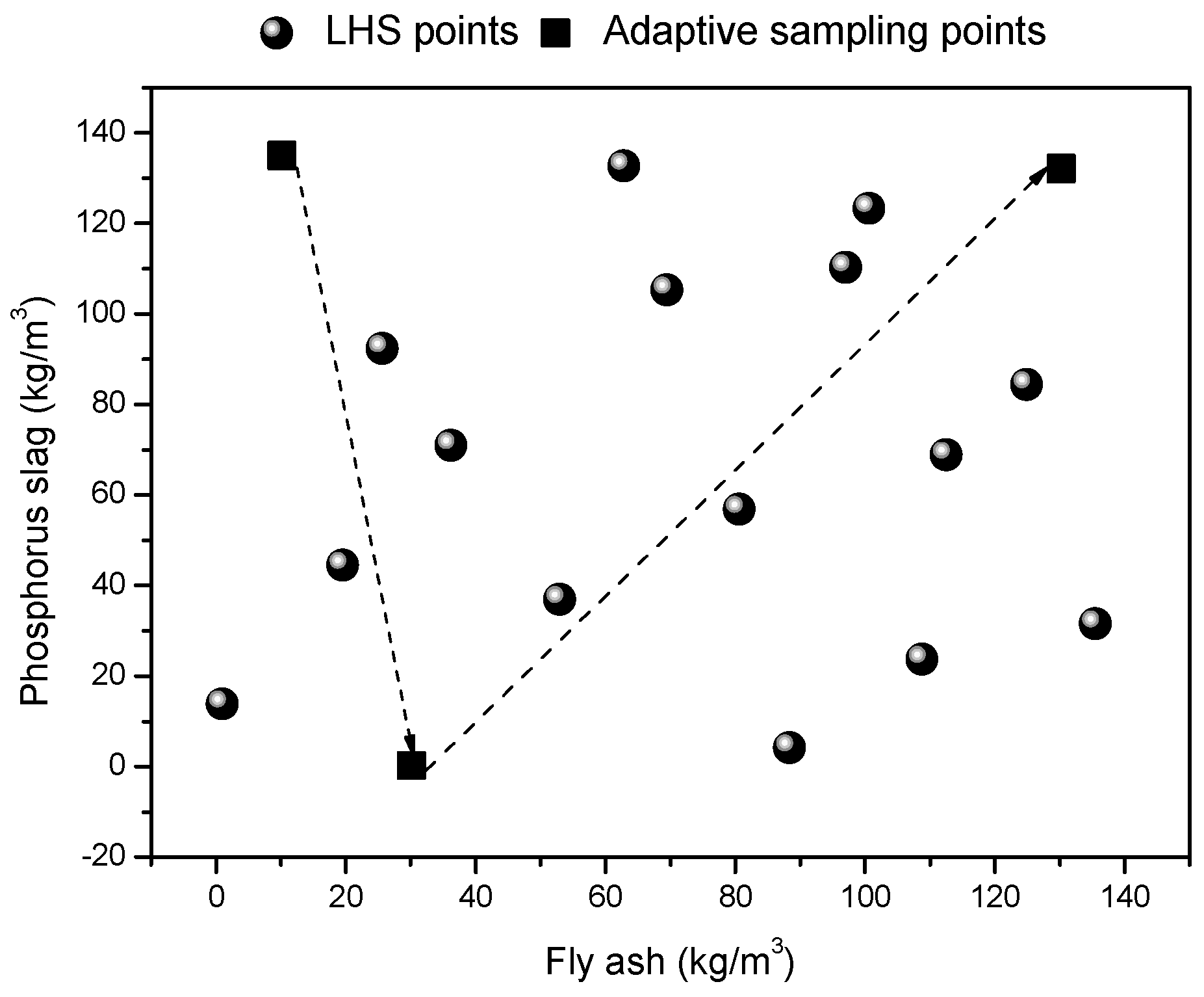
2.1. Latin Hypercube Sampling

The test design is used primarily to determine reasonable methods for acquiring test data. If the arrangement of tests is reasonable and there are few tests required, satisfactory results can be achieved [28]. Usually, the test design includes LHS and orthogonal tests but LHS is more flexible and controllable than the latter for the following reasons. First, the number of experiments can be controlled. Second, LHS design is a space-filled design that allows combinations of input to fill up relatively even test intervals, which ensure more uniformity than in the orthogonal test. Third, LHS design does not get its own test table like orthogonal and uniform experimental design. The main principle is as follows: Let N denote the required number of realizations and K the number of random variables. The sampling space is then K-dimensional. An N × K matrix P, in which each of the K columns is a random permutation of 1, …, N and an N × K matrix R of independent random numbers from the uniform (0,1) distribution is established [29].

2.2. Optimization Methods

GAs, one of the most common optimization methods, are utilized to find optimal solutions by simulating the natural evolution process [30]. However, GAs often finds local advantages, which are “premature.” Multi-island GAs prevents the problem of prematurity because many “islands” are added on the basis of the GA. Some individuals can migrate between the islands. Therefore, multi-island GAs can avoid a local optimum and achieve a global optimum.

2.3. Extended Radial Basis Function Models

Research experiments are generally expensive, and they require a large amount of resources. Hence, design optimization using the ERBF surrogate model can be used to reduce the total number of experiments needed, which is very important to ensure low costs.
ERBF methods are an extension of the RBF. The ERBE approach results in an underdetermined system of linear equations, which yields a family of solutions. This powerful new technique allows the designer more freedom in building metamodels and ultimately results in more accurate and effective metamodels [31], which is expressed in terms of the Euclidean distance ( r = x x i ) from one generic point x to a given data point xi that is defined as:
φ ( r ) = r 2 + c 2 ,
where c denotes a prescribed parameter, which ensures the validity of the Euclidean distance [32]. The RBF is a linear combination equation, which is expressed as:
f ( x k ) = i = 1 n p σ i φ ( x k x i ) , k = 1 , , n p ,
where σ i is an unknown factor to be solved for and n p denotes the number of sample points. The above equations are expressed in the form of a matrix, as shown below:
[ A ] { σ } = { F } ,
where F, σ and Aik are expressed as:
A i k = ϕ ( x k x i ) , i = 1 , , n p , k = 1 , , n p
σ = [ σ 1 σ 2 σ n p ] T ,
F = [ f ( x 1 ) f ( x 2 ) f ( x n p ) ] T ,
where Aik is calculated using the Euclidean distance of point xi and xk. σ is obtained by solving Equation (3). The Euclidean distance between an undiscovered point x and each data point (x1, x2, …, xnp) within the design domain is expressed as:
ε = [ φ ( x x 1 ) φ ( x x 2 ) φ ( x x n p ) ] .
The RBF interpolation results for a generic point x are represented as:
f ( x ) = [ ε ] { σ } .
Typical RBF methods only offer one interpolative solution to the surrogate model. Mullur and Messac (2005) proposed a surrogate model of the ERBF [32], where they defined one coordinate vector as ξ j i = x j x j i , which expresses the coordinate of all the x points within the design domain relative to sample point xi in the jth dimension and the non-RBFs are defined as:
ϕ i j ( ξ j i ) = α i j L ϕ L ( ξ j i ) + α i j R ϕ ( ξ j i ) + β i j L ϕ β ( ξ j i ) .
Table 1 describes the ϕ L ϕ R and ϕ β functions.
Here, n and γ are specified parameters. The ERBF approach serves as one surrogate model method, combining the RBF and the non-RBF, which is expressed as:
f ( x k ) = i = 1 n p σ i φ ( x k x i ) + i = 1 n p ϕ i ( x k x i ) ,
and
f ( x k ) = i = 1 n p σ i φ ( x k x i ) + i = 1 n p j = 1 m { α i j L ϕ L ( ξ j i ) + α i j R ϕ R ( ξ j i ) + β i j L ϕ β ( ξ j i ) } ,
where
α L = { α 11 L , α 12 L α 1 m L α ( n p ) ( m ) L } ( m n p ) ( 1 ) T
α R = { α 11 R , α 12 R α 1 m R α ( n p ) ( m ) R } ( m n p ) ( 1 ) T
β = { β 11 β 12 β 1 m β ( n p ) ( m ) } ( m n p ) ( 1 ) . T
Hence, f(xk) is expressed as:
{ F } = [ A ] { σ } + [ B ] { ( α L ) T ( α R ) T β T } T .
Among the k-th row of B is indicated as:
B k = { B L k , B R k , B β k } ( 1 ) × ( 3 m n p ) .
BLk is expressed as:
B L k = { ϕ L ( x 1 k x 1 1 ) , ϕ L ( x 2 k x 2 1 ) ϕ L ( x m k x m 1 ) ϕ L ( x m k x m n p ) } ( 1 ) × ( m n p ) T .
In addition,
A ¯ = [ A , B ] ,
α ¯ = [ α T , ( α L ) T , ( α R ) T , β T ] T .
Hence, Equation (15) is expressed as:
[ A ¯ ] { α ¯ } = [ F ] .
Vector α ¯ is obtained by solving Equation (20). The Euclidean distance and the non-radial basis value of the sample point x with respect to each data point (x1, x2, …, xnp) is expressed as:
ε ¯ = [ φ ( x x 1 ) , φ ( x x 2 ) φ ( x x n p ) ϕ L ( x 1 x 1 1 ) , ϕ L ( x 2 x 2 1 ) ϕ L ( x m x m 1 ) ϕ L ( x m x m n p ) ϕ R ( x 1 x 1 1 ) , ϕ R ( x 2 x 2 1 ) ϕ R ( x m x m 1 ) ϕ R ( x m x m n p ) ϕ β ( x 1 x 1 1 ) , ϕ β ( x 2 x 2 1 ) ϕ β ( x m x m 1 ) ϕ β ( x m x m n p ) ] [ ( 3 m + 1 ) + n p ] × 1 .
The ERBF interpolation results for generic point x is represented as:
f ( x ) = [ ε ¯ ] { σ ¯ } .
ERBF methods offer the designer remarkable freedom and flexibility compared to traditional RBFs with regard to the process of constructing the surrogate model. In addition, research results demonstrate that ERBF methods have a higher accuracy rate in some research fields.
The normalized root mean squared error (NRMSE) is adopted for measuring the accuracy of the surrogate model. It is defined as:
N R M S E = { K = 1 K [ f ( x k ) f ( x k ) E F A ] 2 K = 1 K [ f ( x k ) E F A ] 2 } 2 × 100 .
The descriptive error measure indicates the error of the adaptive surrogate model. A low NRMSE value suggests a good fit, while a high NRMSE value suggests a bad fit.
In order to decrease the number of experiments required and enhance the surrogate model’s adaptive ability [33], several scholars propose the combination of adaptive sampling and the surrogate model in order to minimize resource costs and the computational time [34]. Chen et al. (2014) enhanced the efficiency of the Kriging surrogate model by utilizing local adaptive sampling methods [22]. A multi-island GA-based adaptive sampling approach was therefore proposed to verify the accuracy of the adaptive surrogate model [24]. Hence, an adaptive surrogate model based on ERBFs and adaptive sampling was selected for use in this study.

2.4. Calculation of Costs and CO2 Emissions

Based on the LCA, the assessment of the costs and CO2 emissions for one concrete mixture is supposed to incorporate the phases of material production, transportation and construction [8,35]. The material production, transportation and construction stages includes the costs and CO2 emissions produced during concrete production, transportation and construction, respectively. Therefore, the concrete costs and CO2 emissions can be expressed as shown in Equations (24) and (25), respectively.
Cost = Cost m + Cost t + Cost c ,
C O 2 = C O 2 m + C O 2 t + C O 2 c ,
where Costm denotes material costs, Costt denotes concrete material transportation costs, Costc denotes concrete construction costs, CO2−m denotes the CO2 emissions during material production, CO2−t denotes the CO2 emissions during material transportation and CO2−c denotes the CO2 emissions during construction.

2.4.1. Material Manufacture

Material Costs represent the money needed for material purchase. In other words, the material costs are calculated based on the amount of material needed and cost per unit, as shown in Equation (26). The carbon emission factor is necessary for assessing CO2 emissions produced during material production. The CO2 emissions are calculated from the product of the CO2 emission factor and the total amount of construction materials used, as shown in Equation (27).
Cost m = ( Q i × U C i ) ,
C O 2 m = ( Q i × E F i ) .
Here, Qi denotes the i material quantity (kg), UCi denotes the i material unit price per unit weight (yuan/kg) and EFi denotes the i material emission factor (kg-CO2/kg).

2.4.2. Transportation

The costs and CO2 emissions of concrete during transportation are calculated on the basis of the equipment used, as shown in Equations (28) and (29).
Cost t = ( T D i × Q i C i × U C j S M j ) ,
C O 2 t = ( T D i × Q i C i × F E j i × E F j ) .
Here, TDi denotes the transportation distance from the construction site to the factory to produce the i materials (km), Qi denotes the quantity of the i materials (kg), Cj denotes average carrying capacity of the vehicle used to transport type i materials (kg), SMj denotes the j vehicle standard movement per hour (km/h), UCj denotes the j vehicle unit cost per unit time ($/h), FEji denotes unit fuel consumption of the j vehicle used to transport type i materials (kg/km) and EFj denotes the j vehicle fuel emission factor (kg-CO2/GJ).

2.4.3. Construction Work

The costs and CO2 emission during construction are calculated on the basis of the equipment used, as shown in Equations (30) and (31).
Cost t = ( P d i × T d i × N i × U C e ) ,
C O 2 t = ( P d i × T d i × N i × E F e )
Here, Pdi denotes electric power of the type i machines and tools (kW); Tdi denotes operating hours of type i machines and tools (h); Ni denotes number of type i machines and tools (units); UCe denotes the electricity unit costs ($/kWh); and EFe denotes the electricity emission factor (kg-CO2/kWh).
EF is the emission factor. Emission factors of different materials and energies are different. The emission factors of materials and energies were obtained through relevant literature, as shown in Table 2.

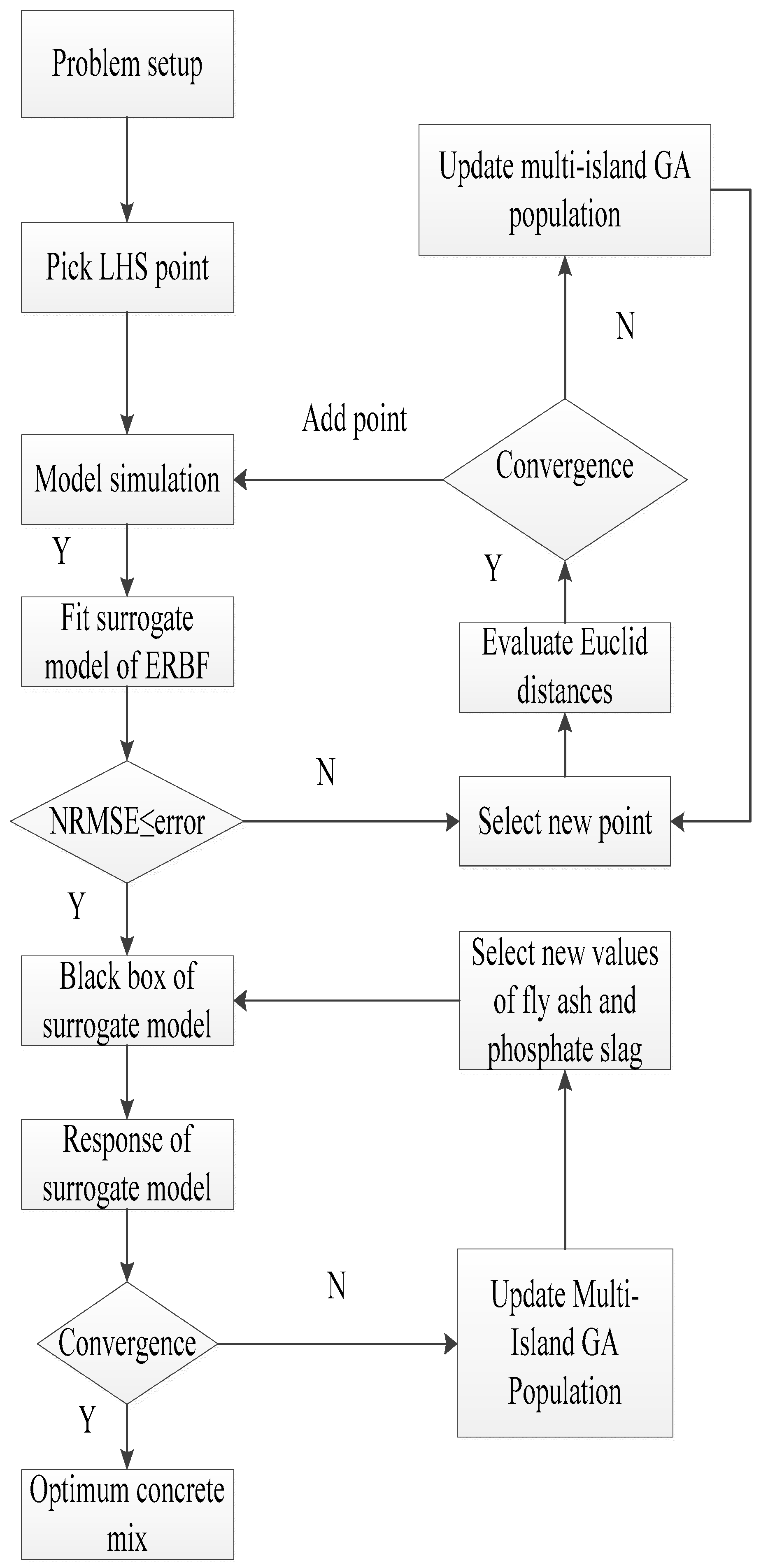
2.5. Concrete Mixture Optimization Algorithm for Adaptive Surrogate Model

The multi-island GA method is combined with an adaptive surrogate modeling approach to achieve concrete mixture optimization. The concrete mixture optimization process is shown in Figure 2. The original sampling points are obtained by employing the LHS method. The results of the original sample point are used to construct the ERBF surrogate model. With regard to the convergence criterion, if the iteration converges based on the standard error measure, the surrogate model black box is constructed if the convergence conditions are met. Otherwise, new points are searched for using the adaptive sampling technique. The Euclidean distance between the new sample point and the selected sample point is assessed. If the iteration converges during the search for a new sample point, this point is appended to the model simulations; else, the population of the multi-island GA is updated. Iteration convergence indicates the end of the process or that the population of the multi-island GA has been updated.

3. Concrete Mixture Optimization Based on Adaptive Surrogate Model

3.1. Problem Definition

The surrogate model was used to find the optimal concrete mixture with the lowest cost and CO2 emission using as little experimental data as possible. Three kinds of concrete mixtures with different strength were selected based on a study at the local concrete mixture station, which will be the basis of the optimal design of concrete mix and the reference objects to the optimal mix, as shown in Table 3.

3.2. Concrete Mixture Optimization Using Surrogate Model

Before the optimization of the concrete mixture using the surrogate model, it is necessary to set up a black box. Fifteen original sample points for each concrete were selected using the LHS method. The new sample points were selected using the adaptive sampling method when the surrogate models did not reach a convergence tolerance of 0.02. The new sample points were placed in the sparsely populated area formed by the original sample points, thereby improving the veracity of the updated surrogate model. That is, the number of sampling points is minimized under the condition that the convergence tolerance of the adaptive surrogate model is a fixed value. Take into account these sample points, the specimens were poured (Figure 3a), placed in 20 °C and 95% RH curing tanks for 28 days (Figure 3b) and tested under various pressures, as shown in Figure 3c,d. The results showed that the adaptive surrogate model had a convergence tolerance of 0.02. 2, 2 and 3 new sample points were added for C70, C40 and C30 concrete respectively, the arrows indicated the order in which new sample points were obtained, as shown in Figure 4, Figure 5 and Figure 6. The sample points of the fly ash and phosphorus slag for the three types of concrete are listed in Table 4. When the total amount of cementitious material is constant, the replacement rate of cement with fly ash and phosphorous slag is within 38%.
This adaptive sampling method requires a minimum number of sample points of concrete to satisfy a surrogate model error of 0.02. The experimental results of the pressure strength, CO2 emissions and cost of the three strength concrete sample points for 28 days are shown in Table 5, where Fcu,k = 70 stands for that design strength is C70, Fcu,k = 40 stands for that design strength is C40,Fcu,k = 30 stands for that design strength is C30. Not all concrete can achieve the required compressive strength due to the mix has changed, CO2 emissions and costs of sample points of the three strength concretes are different, which lays a foundation for establishment of surrogate model.
A surrogate model based on the sample points of the 3 types of concrete with different strength was constructed to optimize the concrete mixture with the lowest carbon emissions and cost. The multi-island GA was used to select the values of fly ash and phosphate slag; then, the optimal concrete mixture with the lowest CO2 emissions and cost was obtained using the surrogate model black box based on these values. Finally, if the result does not converge, the group in the multi-island GA is updates and the range of fly ash and phosphate slag is selected; however, the optimal concrete mixture was obtained. The objective function of this optimization problem is as follows:
M a x : F 1 S T . : 0 x 1 209 ,   0 x 2 159.6 ,   0 x 3 136.8 0 y 1 209 ,   0 y 2 159.6 ,   0 y 3 136.8
Here, F1 is the lowest CO2 emission and cost; x and y are the design variables; x1, x2 and x3 respectively represent the fly ash values for the concrete mixtures with intensities of 70, 40 and 30; and y1, y2 and y3 respectively represent the phosphorus slag values for the concrete mixtures with intensities of 70, 40 and 30. The strength requirement must be met as a boundary condition.

4. Discussion

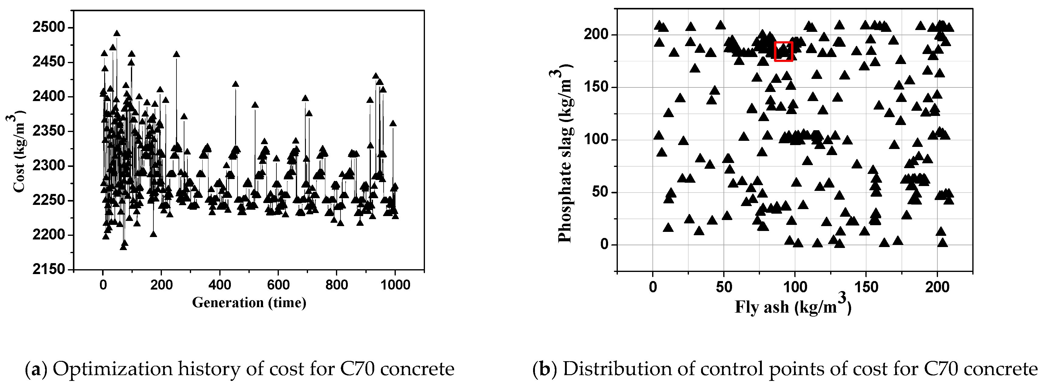
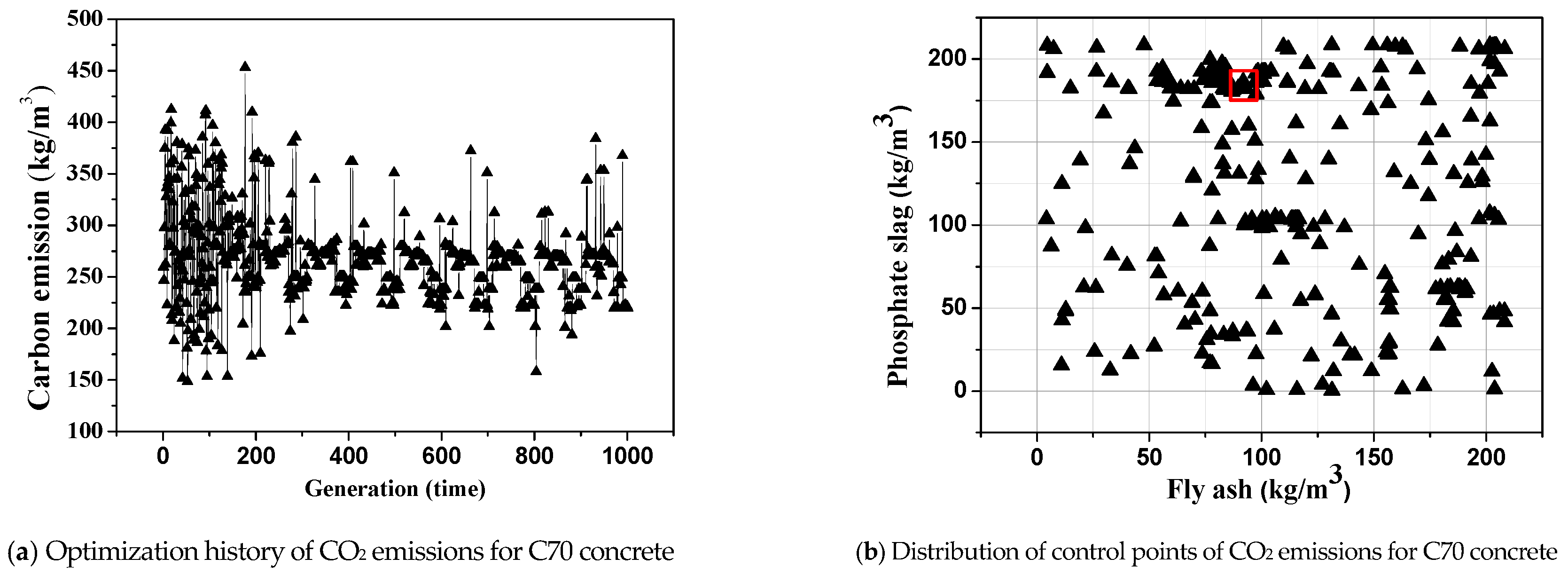
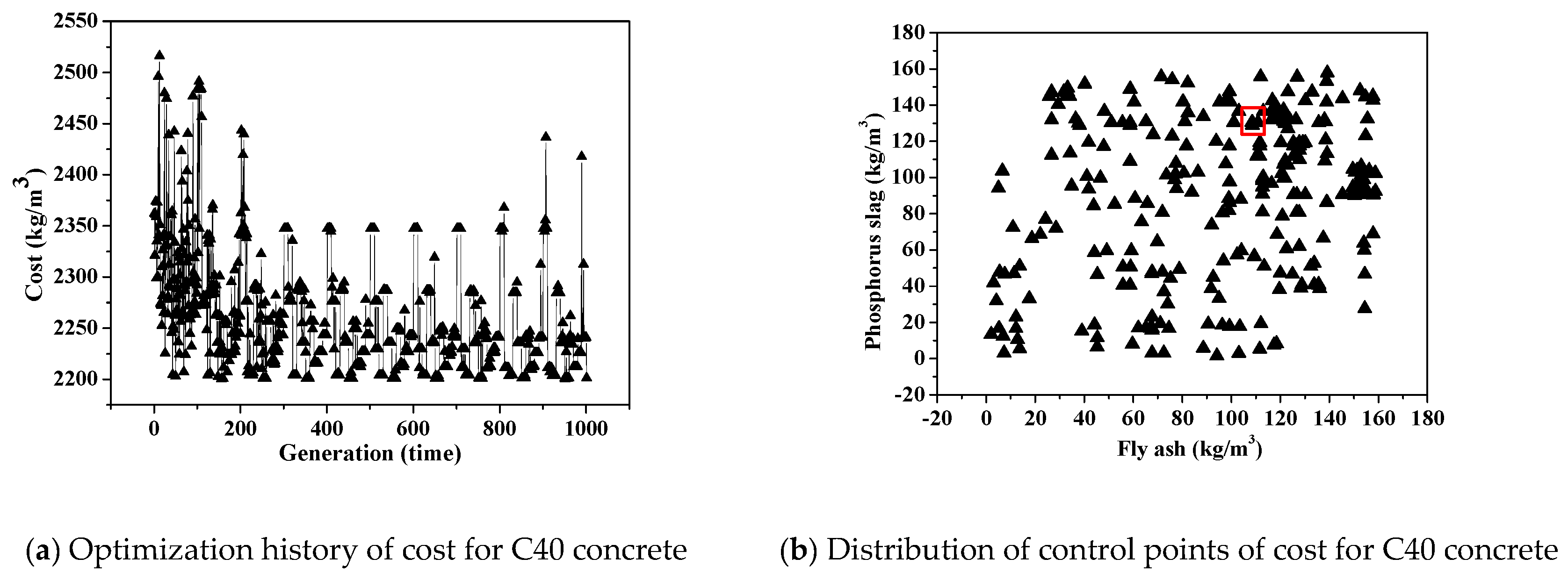
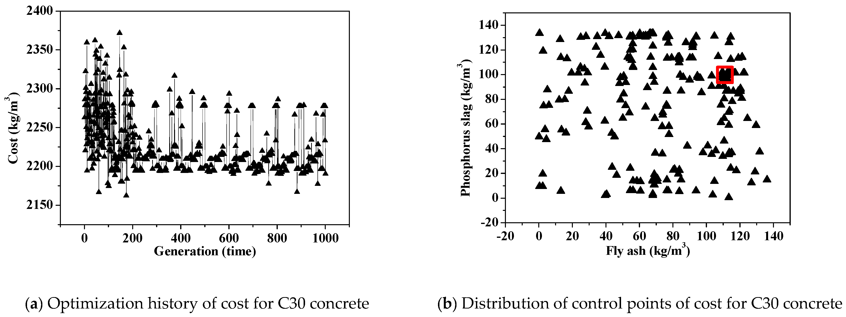
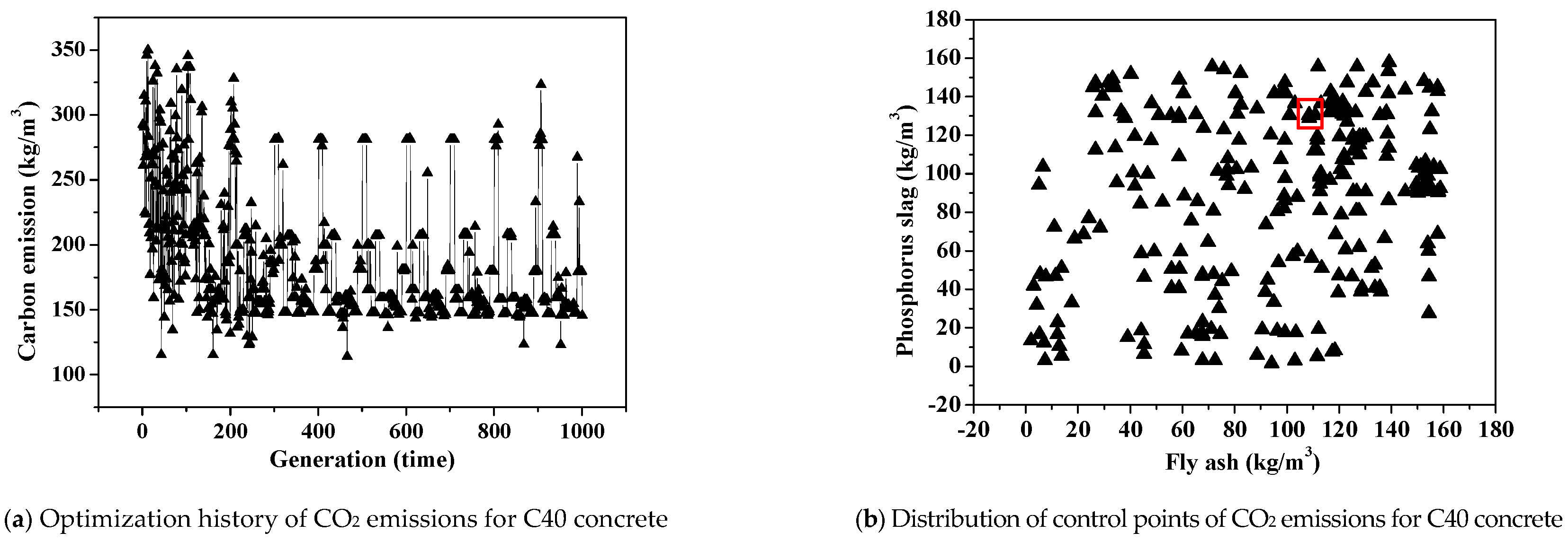
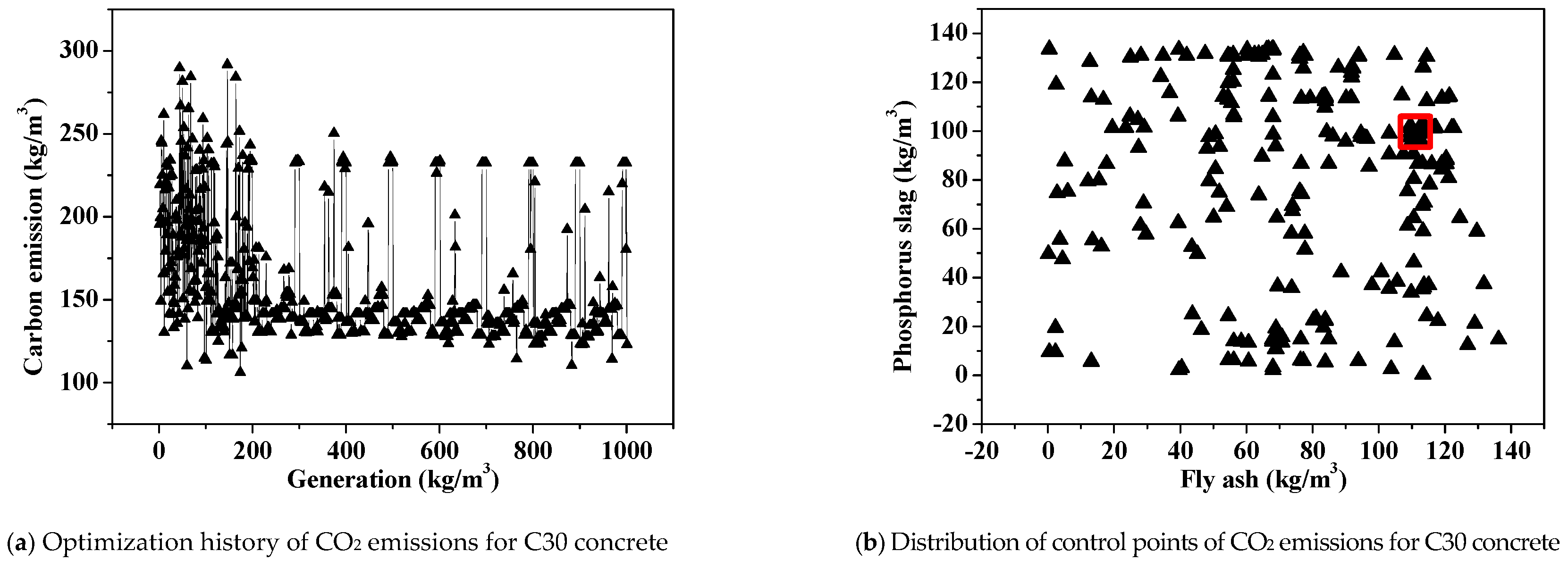
4.1. Optimization History of CO2 Emissions and Cost for Each Type of Concrete and Distribution of Control Points

The optimal value tends to be stable as the number of iterations increases. There are 10 islands in the multi-island GA due to the existence of 10 locally optimal solutions. However, there is just one globally optimal solution. When the boundary condition is satisfied, the minimum stable value of the generation process represents the optimal value.
Figure 7a shows optimization history of the cost of C70 concrete. Iteration reaches the 1001st time, the optimal cost is 2233.16 yuan/m3. The optimum point is indicated by the red circle in Figure 6b. The optimal values of fly ash and phosphorus slag are 99.27 kg/m3 and 191.61 kg/m3, respectively.
Figure 8a shows optimization history of the CO2 emissions for C70 concrete. The optimal value of CO2 emissions is 219.95 kg/m3 when generation time is 1001. The optimum point is shown as the red circle in Figure 8b. The optimal values of fly ash and phosphorus slag are 99.27 kg/m3 and 191.61 kg/m3, respectively.
Figure 9a shows the optimization history of C40 concrete cost, the number of iterations is 1002 and the optimum cost is 2226.95 yuan/m3. The optimum point is shown as the red circle in Figure 9b. The optimal values of fly ash and phosphorus slag are 152.99 kg/m3 and 103.01 kg/m3, respectively.
Figure 10a shows the CO2 emissions optimization history of C40 concrete. The minimum stable value of the CO2 emissions is 148.09 kg/m3 after generation time is 1002. The optimum point is indicated by the red circle in Figure 10b. The optimal values of fly ash and phosphorus slag are 152.99 kg/m3 and 103.01 kg/m3, respectively.
Figure 11a shows the cost optimization history of C30 concrete. When the number of iterations is 1001, the optimal cost is 2194.23 yuan/m3. The optimum point is indicated by the red circle in Figure 11b. The optimal values of fly ash and phosphorus slag are 113.56 kg/m3 and 101.39 kg/m3, respectively.
Figure 12a shows the CO2 emissions optimization history of C30 concrete, generation time is 1001 and the minimum value of CO2 emissions is 130.33 kg/m3. The optimum point is indicated by the red circle in Figure 12b. The optimal values of fly ash and phosphorus slag are 113.56 kg/m3 and 101.39 kg/m3, respectively.

4.2. Comparison of Reference and Optimal Mixtures of Concrete

Concrete mixture from the Kaili concrete plant was used as the reference sample, which was compared with the optimal concrete mixture based on the surrogate model, comparison of reference and optimal mixtures of concrete is shown in Table 6.
For C70 concrete, the fly ash in the optimized mixture decreased by 0.73 kg/m3, the phosphorus slag increased by 91.61 kg/m3 and the cement decreased by 90.88 kg/m3 compared with those of the reference sample. However, the CO2 emissions decreased by 553.61 kg/m3 and the cost decreased by 93.6 yuan/m3 compared with those of the reference sample, respectively.
For C40 concrete, the fly ash in the optimal concrete mixture increased by 92.99 kg/m3, the phosphorus slag increased by 53.01 kg/m3 and the cement decreased by 146 kg/m3 compared with those of the reference sample. However, the CO2 emissions decreased by 113.51 kg/m3 and the cost decreased by 126.56 yuan/m3 compared with those of the reference sample.
For C30 concrete, the fly ash in the optimized mixture increased by 53.56 kg/m3, the phosphorus slag increased by 41.39 kg/m3 and the cement decreased by 94.95 kg/m3 compared with those of the reference sample. However, the CO2 emissions decreased by 75.17 kg/m3 and the cost decreased by 78.68 yuan/m3 compared with those of the reference sample, respectively.

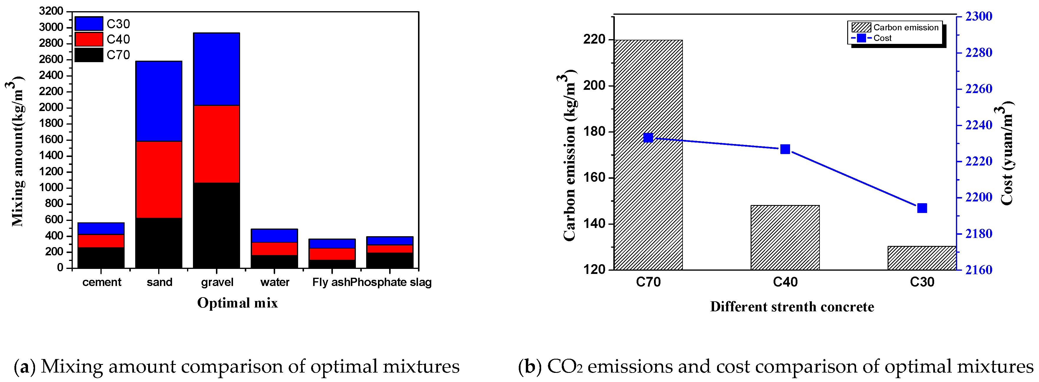
4.3. Comparison of Optimal Mixtures of Concrete

Based on a comparison of the three types of concrete, it was found that the CO2 emissions and cost increase with increasing strength, which is consistent with a previous study [11]. Figure 13a shows that the cement content varies greatly and C70 concrete has the highest amount of cement, which results in higher CO2 emissions. The carbon dioxide emissions of the optimized mix C70, C40 and C30 concrete are quite different, which are respectively 219.95 kg/m3, 148.09 kg/m3 and 130.33 kg/m3. The cost difference between the three types of concrete is not significant. Although the cost of C70 is the highest, the difference is less than 0.3%, as shown in Figure 13b. Therefore, the amount of cement plays a key role in the concrete CO2 emissions and the optimal mix is of great significance to reduce the carbon emission of concrete.
This work showed that optimization of concrete mixture design using adaptive surrogate model can reduce CO2 emissions and cost of concrete. Before concrete production, this method can be used to find the optimal mix with the lowest carbon emission and cost, which not only reduces the damage to the environment but also can make better use of fly ash and phosphorus slag. On this basis, the optimal mix ratio system of concrete can also be built, which will beneficial to decrease the environmental burden of global concrete [41].

5. Conclusions

This paper reported the optimizing design of a concrete mixture in order to reduce its CO2 emissions and cost using an adaptive surrogate model. From a sustainability perspective, this paper provides a technological approach to reducing concrete carbon emissions, which has implications for decreasing the environmental burden of concrete. In addition, based on a comparison of concrete optimal mix, it was found that optimized concrete’s CO2 emissions were less than the reference samples and the reduction of carbon emissions did not lead to an increase in costs. In this way, we can optimize concrete of different strength to reduce carbon dioxide emission and establish optimized mix system of concrete. It is possible to verify that optimization of concrete mixture design using adaptive surrogate model is a sustainable method and a feasible path to improve the environmental performance of the concrete industry. The major contributions of this study are as follows:
First, the adaptive surrogate model was utilized to optimize concrete mixtures by using an objective function based on the CO2 emissions and lowest cost and the amount of fly ash and phosphorous slag were used as the design variables. Fifteen original sample points of three types of concrete with different strength were selected using the LHS method. New sample points numbering 2, 2 and 3 were added based on the adaptive sampling method for C70, C40 and C30 concrete, respectively, to meet the 0.02 error tolerance range of the surrogate model.
Second, the results show that fly ash and phosphorous slag have a significant influence on the CO2 emissions but have little effect on cost. The cost and CO2 emissions of C70, C40 and C30 concrete are the lowest when the values of fly ash and phosphorus slag are 99.27 kg/m3, 152.99 kg/m3 and 113.56 kg/m3 and 191.61 kg/m3, 101.39 kg/m3 and 103.01 kg/m3, respectively.
Third, based on a comparison of the concrete mixture from the Kaili concrete plant, which was used as a reference sample and the optimal concrete mixture based on the surrogate model, optimized concrete’s cost and CO2 emissions were less than the reference sample’s. It was found that the cost of the optimized concrete decreased by 93.60 yuan/m3, 126.56 yuan/m3 and 78.68 yuan/m3 and the CO2 emissions decreased by 553.61 kg/m3, 113.51 kg/m3 and 75.17 kg/m3 for C70, C40 and C30 concrete, respectively, compared with those of the reference sample.
In addition, this paper also has a few deficiencies. In the optimization, only the strength requirement as a mechanical property which must be met is incomplete. In fact, there are also other mechanical properties. For instance, dissipative behavior must be affected by the particular mixture adopted or the swelling potential, shrinkage limits [42,43]. Those experimental studies will be drawn up and presented in a further work.

Author Contributions

X.C. developed the concept and drafted the manuscript, Q.W. and X.S. revised the manuscript and supervised the overall work. Y.S. and J.Q. participated in experiments and data analysis.

Funding

This study was funded by the Program for Changjiang Scholars and Innovative Research Team (Project No. IRT14R37), the National Natural Science Foundation of China (Project No. 51208325) and the Science and Technology Joint Foundation of Guizhou Technology Hall, Qiandongnan Technology Bureau and Kaili University in China (Project No. [2016] 7321).

Acknowledgments

The research was conducted using data for the case study provided by the Kaili concrete mixture station.

Conflicts of Interest

The authors declare that they have no conflicts of interest.

References

  1. Chunzhi, Z.; Yi, L.; Shiwei, R.; Jiang, Q. Study on Carbon Emission Calculation Method of Concrete. Key Eng. Mater. 2018, 768, 293–305. [Google Scholar]
  2. Bosoaga, A.; Masek, O.; Oakey, J.E. CO2 Capture Technologies for Cement Industry. Energy Proced. 2009, 1, 133–140. [Google Scholar] [CrossRef]
  3. Deja, J.; Uliasz-Bochenczyk, A.; Mokrzycki, E. CO2 emissions from Polish cement industry. Int. J. Greenh. Gas Control 2010, 4, 583–588. [Google Scholar] [CrossRef]
  4. Monteiro, P.J.M.; Miller, S.A.; Horvath, A. Towards sustainable concrete. Nat. Publ. Gr. 2017, 16, 698–699. [Google Scholar] [CrossRef]
  5. Miller, S.A. Supplementary cementitious materials to mitigate greenhouse gas emissions from concrete: Can there be too much of a good thing? J. Clean. Prod. 2018, 178, 587–598. [Google Scholar] [CrossRef]
  6. Yang, K.; Jung, Y.; Cho, M.; Tae, S. Effect of supplementary cementitious materials on reduction of CO2 emissions from concrete. J. Clean. Prod. 2015, 103, 774–783. [Google Scholar] [CrossRef]
  7. Vargas, J.; Halog, A. Effective carbon emission reductions from using upgraded fly ash in the cement industry. J. Clean. Prod. 2015, 103, 948–959. [Google Scholar] [CrossRef]
  8. Peng, C. Calculation of a building’s life cycle carbon emissions based on Ecotect and building information modeling. J. Clean. Prod. 2016, 112, 453–465. [Google Scholar] [CrossRef]
  9. Mclellan, B.C.; Williams, R.P.; Lay, J.; van Riessen, A.; Corder, G.D. Costs and carbon emissions for geopolymer pastes in comparison to ordinary portland cement. J. Clean. Prod. 2011, 19, 1080–1090. [Google Scholar] [CrossRef]
  10. Sandanayake, M.; Gunasekara, C.; Law, D.; Zhang, G.; Setunge, S. Greenhouse gas emissions of different fly ash based geopolymer concretes in building construction. J. Clean. Prod. 2018, 204, 399–408. [Google Scholar] [CrossRef]
  11. Kim, T.; Tae, S.; Roh, S. Assessment of the CO2 emission and cost reduction performance of a low-carbon-emission concrete mix design using an optimal mix design system. Renew. Sustain. Energy Rev. 2013, 25, 729–741. [Google Scholar] [CrossRef]
  12. Park, H.S.; Kwon, B.; Shin, Y.; Kim, Y.; Hong, T.; Choi, S.W. Cost and CO2 Emission Optimization of Steel Reinforced Concrete Columns in High-Rise Buildings. Energies 2013, 5609–5624. [Google Scholar] [CrossRef]
  13. Camp, C.V.; Assadollahi, A. CO2 and cost optimization of reinforced concrete footings using a hybrid big bang-big crunch algorithm. Struct. Multidiscip. Optim. 2013, 48, 411–426. [Google Scholar] [CrossRef]
  14. Le, K.N.; Tran, C.N.N.; Tam, V.W.Y. Life-cycle greenhouse-gas emissions assessment: An Australian commercial building perspective. J. Clean. Prod. 2018, 199, 236–247. [Google Scholar] [CrossRef]
  15. Hong, T.; Ji, C.; Park, H. Integrated model for assessing the cost and CO2 emission (IMACC) for sustainable structural design in ready-mix concrete. J. Environ. Manage. 2012, 103, 1–8. [Google Scholar] [CrossRef] [PubMed]
  16. Esmaeilkhanian, B.; Khayat, K.H.; Wallevik, O.H. Mix design approach for low-powder self-consolidating concrete: Eco-SCC—Content optimization and performance. Mater. Struct. Constr. 2017, 50, 1–18. [Google Scholar] [CrossRef]
  17. Chkifa, A.; Cohen, A.; Migliorati, G.; Nobile, F.; Tempone, R. Discrete least squares polynomial approximation with random evaluations—Application to parametric and stochastic elliptic PDEs. ESAIM Math. Model. Numer. Anal. 2015, 49, 815–837. [Google Scholar] [CrossRef]
  18. Audet, C.; Denni, J.; Moore, D.; Booker, A.; Frank, P. A surrogate-model-based method for constrained optimization. In Proceedings of the 8th Symposium on Multidisciplinary Analysis and Optimization, Long Beach, CA, USA, 6–8 September 2000. [Google Scholar]
  19. Wu, Z.; Huang, D.; Wang, W.; Chen, T.; Lin, M.; Xie, Y.; Niu, M.; Wang, X. (Alice) Optimization for fire performance of ultra-low density fiberboards using response surface methodology. BioResources 2017, 12, 3790–3800. [Google Scholar] [CrossRef]
  20. Akhtar, T.; Shoemaker, C.A. Multi objective optimization of computationally expensive multi-modal functions with RBF surrogates and multi-rule selection. J. Glob. Optim. 2016, 64, 17–32. [Google Scholar] [CrossRef]
  21. Benner, P.; Gugercin, S.; Willcox, K. A Survey of Projection-Based Model Reduction Methods for Parametric Dynamical Systems. SIAM Rev. 2015, 57, 483–531. [Google Scholar] [CrossRef]
  22. Chen, Z.; Qiu, H.; Gao, L.; Li, X.; Li, P. A local adaptive sampling method for reliability-based design optimization using Kriging model. Struct. Multidiscip. Optim. 2014, 49, 401–416. [Google Scholar] [CrossRef]
  23. Remondo, D.; Srinivasan, R.; Nicola, V.F.; Van Etten, W.C.; Tattje, H.E.P. Adaptive importance sampling for performance evaluation and parameter optimization of communication systems. IEEE Trans. Commun. 2000, 48, 557–565. [Google Scholar] [CrossRef]
  24. Vytla, V.V.; Huang, P.G.; Penmetsa, R.C. Multi objective aerodynamic shape optimiaztion of high speed train nose using adaptive surrogate model. In Proceedings of the 28th AIAA Applied Aerodynamics Conference, Chicago, IL, USA, 28 June–1 July 2010. [Google Scholar]
  25. Guo, S.; Zheng, X.; Ang, H. Structure modal optimization of a strapdown inertial navigation system for an electric helicopter using an adaptive surrogate model. J. Vibroeng. 2017, 19, 5310–5326. [Google Scholar]
  26. Van den Heede, P.; De Belie, N. Environmental impact and life cycle assessment (LCA) of traditional and ‘green’ concretes: Literature review and theoretical calculations. Cem. Concr. Compos. 2012, 34, 431–442. [Google Scholar]
  27. Peng, W.; Pheng, L.S. Managing the Embodied Carbon of Precast Concrete Columns. J. Mater. Civ. Eng. 2011, 1192–1199. [Google Scholar] [CrossRef]
  28. Toufigh, V.; Pahlavani, H. Probabilistic-Based Analysis of MSE Walls Using the Latin Hypercube Sampling Method. Int. J. Geomech. 2018, 18, 04018109. [Google Scholar] [CrossRef]
  29. Olsson, A.; Sandberg, G.; Dahlblom, O. On Latin hypercube sampling for structural reliability analysis. Struct. Saf. 2003, 25, 47–68. [Google Scholar] [CrossRef]
  30. Wang, S. Research on the EIA of Ready-Mixed Concrete during the Life Cycle; Tsinghua University: Beijing, China, 2009. [Google Scholar]
  31. Xiang, H.; Li, Y.; Liao, H.; Li, C. An adaptive surrogate model based on support vector regression and its application to the optimization of railway wind barriers. Struct. Multidiscip. Optim. 2017, 55, 701–713. [Google Scholar] [CrossRef]
  32. Mullur, A.A.; Messac, A. Extended Radial Basis Functions: More Flexible and Effective Metamodeling. AIAA J. 2005, 43, 1306–1315. [Google Scholar] [CrossRef]
  33. Hardy, R.L. Multiquadric equations of topography and other irregular surfaces. J. Geophys. Res. 1971, 76, 1905–1915. [Google Scholar] [CrossRef]
  34. Proverbio, M.; Costa, A.; Smith, I.F.C.; Asce, F. Adaptive Sampling Methodology for Structural Identification Using Radial-Basis Functions. J. Comput. Civ. Eng. 2018, 32, 1–17. [Google Scholar] [CrossRef]
  35. Turner, L.K.; Collins, F.G. Carbon dioxide equivalent (CO2−e) emissions: A comparison between geopolymer and OPC cement concrete. Constr. Build. Mater. 2013, 43, 125–130. [Google Scholar] [CrossRef]
  36. Li, C.; Nie, Z.; Cui, S.; Gong, X.; Wang, Z.; Meng, X. The life cycle inventory study of cement manufacture in China. J. Clean. Prod. 2014, 72, 204–211. [Google Scholar] [CrossRef]
  37. Kawai, K.; Sugiyama, T.; Kobayashi, K.; Sano, S. Inventory Data and Case Studies for Environmental Performance Evaluation of Concrete Structure Construction. J. Adv. Concr. Technol. 2005, 3, 435–456. [Google Scholar] [CrossRef]
  38. Chen, C.; Habert, G.; Bouzidi, Y.; Jullien, A.; Ventura, A. LCA allocation procedure used as an incitative method for waste recycling: An application to mineral additions in concrete. Resour. Conserv. Recycl. 2010, 54, 1231–1240. [Google Scholar] [CrossRef]
  39. Crossin, E. The greenhouse gas implications of using ground granulated blast furnace slag as a cement substitute. J. Clean. Prod. 2015, 95, 101–108. [Google Scholar] [CrossRef]
  40. China Architecture Design and Research Group. Standard for Measuring, Accounting and Reporting of Carbon Emission from Buildings; China Planning Press: Beijing, China, 2014; pp. 73–76. [Google Scholar]
  41. Kim, T.; Chae, C.; Kim, G.; Jang, H. Analysis of CO2 Emission Characteristics of Concrete Used at Construction Sites. Sustainability 2016, 8, 348. [Google Scholar] [CrossRef]
  42. Giorgio, I.; Scerrato, D. Multi-scale concrete model with rate-dependent internal friction. Eur. J. Environ. Civ. Eng. 2016, 21, 821–839. [Google Scholar] [CrossRef]
  43. Misra, A.; Biswas, D.; Upadhyaya, S. Physico-mechanical behavior of self-cementing class C fly ash-clay mixtures. Fuel 2005, 84, 1410–1422. [Google Scholar] [CrossRef]
Figure 1. Concrete output and year over year growth in China in the period 2006–2017 (data from China concrete net).
Sustainability 11 01991 g001
Figure 2. Flow chart of concrete mixture optimization process.
Sustainability 11 01991 g002
Figure 3. Image of experimental process: (a) pouring the concrete specimens; (b) curing the concrete specimens; (c) the concrete specimens before pressure test; (d) the concrete specimens after pressure test.
Sustainability 11 01991 g003
Figure 4. Distribution of sampling points of C70 concrete.
Sustainability 11 01991 g004
Figure 5. Distribution of sampling points of C40 concrete.
Sustainability 11 01991 g005
Figure 6. Distribution of sampling points of C30 concrete.
Sustainability 11 01991 g006
Figure 7. Optimization history of cost for C70 concrete and distribution of control points.
Sustainability 11 01991 g007
Figure 8. Optimization history of CO2 emissions for C70 concrete and distribution of control points.
Sustainability 11 01991 g008
Figure 9. Optimization history of cost for C40 concrete and distribution of control points.
Sustainability 11 01991 g009
Figure 10. Optimization history of CO2 emissions for C40 concrete and distribution of control points.
Sustainability 11 01991 g010
Figure 11. Optimization history of cost for C30 concrete and distribution of control points.
Sustainability 11 01991 g011
Figure 12. Optimization history of CO2 emissions for C30 concrete and distribution of control points.
Sustainability 11 01991 g012
Figure 13. Comparison of optimal mixtures of C30, C40 and C70 concrete.
Sustainability 11 01991 g013
Table 1. Description of non-radial basis functions.
ξ j i ϕ L ϕ R ϕ β
ξ j i γ ( n γ n 1 ) ξ j i + γ n ( 1 n ) 0 ξ j i
γ ξ j i 0 ( ξ j i ) n 0 ξ j i
0 ξ j i γ 0 ( ξ j i ) n ξ j i
ξ j i γ 0 ( n γ n 1 ) ξ j i + γ n ( 1 n ) ξ j i
Table 2. Different materials and energy emission factors.
Materials and Energy NameEmission FactorUnitSource of Date
Cement0.604kgCO2/kg(Li, 2014) [36]
Coarse aggregate2.9 × 10−3kgCO2/kg(Kawai et al., 2005) [37]
Fine aggregate3.7 × 10−3kgCO2/kg(Kawai et al., 2005) [37]
Water0.213 × 10−3kgCO2/kg(Wang, 2009) [30]
Fly ash0.350 × 10−3kgCO2/kg(Chen et al., 2010) [38]
Phosphorous slag0.320 × 10−3kgCO2/kg(Crossin, 2015) [39]
Diesel74.1KgCO2/GJ(CECS374: 2014) [40]
South China power grid0.714KgCO2/(kWh)(CECS374: 2014) [40]
Table 3. Common mixtures at Kaili concrete mixture station.
StrengthCementitious Material (kg/m3)Cement (kg/m3)Fly Ash (kg/m3)Phosphorous Slag (kg/m3)Water (kg/m3)Water Cement RatioWater-Reducing Agent (kg/m3)Sand (kg/m3)Gravel (kg/m3)
C705503501001001600.294.46251065
C4042031060501650.467.6960970
C3036024060601650.4661000900
Table 4. Sample points determined using Latin hypercube sampling.
NumberC70C40C30
Fly Ash (kg/m3)Percentage (%)Phosphorus Slag (kg/m3)Percentage (%)Fly Ash (kg/m3)Percentage (%)Phosphorus Slag (kg/m3)Percentage (%)Fly Ash (kg/m3)Percentage (%)Phosphorus Slag (kg/m3)Percentage (%)
111.392.07193.7235.2223.555.6126.166.231.000.2813.833.84
2191.7234.86169.7330.86136.3532.46128.2130.5397.0426.96110.2530.62
3196.6535.7530.415.530.890.21100.7223.98135.5037.6431.568.77
4180.7432.86115.3320.9782.5819.6695.0722.64124.9134.7084.3923.44
521.053.8325.774.69104.9624.9935.938.5625.607.1192.3625.66
667.3212.244.740.86114.1027.17125.5429.8952.9614.7136.9110.25
769.9712.72132.1124.0215.163.61115.3427.4680.6022.3956.8815.80
8115.4721.0056.1210.2064.7515.4265.4715.59100.6027.94123.3434.26
948.768.8746.698.4951.3512.2391.0621.6819.565.4344.4812.35
10146.7026.67197.8435.9799.3123.6481.6919.45108.8030.2223.706.58
1140.967.4591.2116.5874.9617.857.581.80112.5431.2668.9019.14
12101.9718.54105.4419.17124.1329.5548.8011.6262.8417.45132.6736.85
1396.9317.62155.7128.3143.4010.3311.572.7536.1910.0571.0219.73
14166.2030.22152.1127.6660.1614.3239.699.4569.4719.30105.2829.24
15132.0724.0181.7414.8635.608.4859.7314.2288.3624.544.141.15
1670.1012.75209.5038.090.500.12158.3037.6910.202.83135.0037.50
170.500.09145.3026.42110.3026.2645.6010.86130.2036.17132.1036.69
18////////30.108.360.2000.06
Table 5. Compressive strength, CO2 emissions and cost of concrete for 28 days.
NumberFcu,k = 70Fcu,k = 40Fcu,k = 30
Fcu,1Cost (yuan/m3)CO2 Emissions (kg/m3)Fcu,2Cost (yuan/m3)CO2 Emissions (kg/m3)Fcu,3Cost (yuan/m3)CO2 Emissions (kg/m3)
176.182324.66289.6942.312334.63261.3843.662357.84287.44
247.802205.84168.6252.922260.79185.5034.422211.57137.49
373.292307.98273.8448.042287.75213.5732.382236.79168.67
462.112255.53219.7146.412259.28184.1433.462210.06136.12
570.212444.96413.6659.792328.69254.9155.112279.46206.89
677.112425.77394.2359.322350.03277.0951.882300.81229.08
776.652326.96292.4859.612313.86240.0349.352259.64191.95
880.512350.13316.6838.932205.82129.3129.602188.70123.53
978.032406.70375.7760.532369.60297.0748.672317.32249.01
1065.172215.79181.5033.572207.31130.6532.982242.03193.77
1174.532380.09346.9935.782219.39142.9227.672220.43156.84
1272.942322.91288.5449.592269.80194.4834.382217.41146.43
1365.232288.54253.1047.872336.85263.4040.322283.88215.33
1453.522238.63202.2058.712285.65210.7739.092232.55162.71
1568.282318.05283.7536.872348.04275.2936.162298.82227.28
1689.582302.67273.7863.822482.92239.7543.242268.51186.09
1776.112422.70384.2544.842272.38223.1223.322158.7593.77
18//////32.212360.55276.30
Table 6. Comparison of reference and optimal mixtures of concrete.
ItemC70C40C30
Reference MixOptimal MixReference MixOptimal MixReference MixOptimal Mix
Cement (kg/m3)350.00259.12310.00164.00240.00145.05
Sand (kg/m3)625.00625.00960.00960.001000.001000.00
Gravel (kg/m3)1065.001065.00970.00970.00900.00900.00
Water (kg/m3)160.00160.00165.00165.00165.00165.00
Fly ash (kg/m3)100.0099.2760.00152.9960.00113.56
Phosphate slag (kg/m3)100.00191.6150.00103.0160.00101.39
Carbon emission (kg/m3)773.56219.95261.60148.09205.50130.33
Cost (yuan/m3)2326.762233.162353.512226.952272.912194.23

