The Sustainability Performance of Chinese Banks: A New Network Data Envelopment Analysis Approach and Panel Regression

Abstract

This paper develops a new network data envelopment analysis (DEA) model that simultaneously integrates the non-convex metafrontier and undesirable outputs and which is super efficient at performing dynamic network slacks-based measures. The model is employed to discuss the efficiency of 36 commercial banks in China during the years 2010–2014. The efficiency of these banks shows significant heterogeneity and the efficiency of most foreign banks has much room for improvement. Regarding both the non-convex metafrontier and the group frontier, state-owned banks perform the best, followed by joint-stock banks, with foreign banks performing the worst; the same is true for the technology gap ratios. The empirical results produced by the feasible generalized least squares estimation method indicate that liquidity and scale effects exert positive impacts on bank efficiency. An alternative estimation method confirmed that the conclusions were robust.

1. Introduction

Commercial banks play a central role in a healthy financial system, especially in developing countries, such as China, where bank performance and stability are vital to the development of the whole economy. According to the China Banking Regulatory Commission, at the end of December 2016, the total assets and liabilities of banking institutions reached 226.26 and 208.92 trillion RMB, respectively, corresponding to 77.80% (assets) and 78.00% (liabilities) of all financial institutions and grew by 15.8% and 16%, respectively, over the previous year. Specifically, in terms of total assets and total liabilities, the year-on-year growth rate of banking institutions of various sizes is more than 14%, ranging from 14.1% to 17.5%. Among these institutions, commercial banks have the lowest growth rate (10% or less), while joint-stock commercial banks are slightly higher, and the growth rate of city commercial banks is more than 20%. These observations imply that the performance of different commercial banks varies. Furthermore, competition among Chinese banks, along with competition between domestic and foreign banks, has become fierce [1]. To increase competitiveness, it is therefore necessary to improve bank performance in China. The reasons can be analyzed from at least three perspectives, as follows. First, improvement of the bank efficiency will help to alleviate the shocks from foreign banks entering China’s financial markets. Second, improving the efficiency of commercial banks is an important part of banking reform in China. Finally, the inefficiency of commercial banks will have a significant impact on the sustainable development of the banking industry. Based on these facts, this study seeks to explore the performance of Chinese banks and investigate its determinants.

Numerous studies on the issues of bank efficiency apply either data envelopment analysis (DEA) or stochastic frontier analysis (SFA). Based on the main advantages of these two methods, a Stochastic Nonparametric Envelopment of Data has been proposed by [2,3]. This method integrates DEA and SFA into a unified framework of productivity analysis. Though SFA, one can separate the effects of random errors on the estimated efficiency scores. SFA requires exact specification of the functional forms of the frontier and the inefficiency distribution [4]. However, a DEA (radial or non-radial, oriented or non-oriented) model has several advantages, such as its nonparametric treatment of the frontier, no requirement for specifying a functional form and it considers price information. A DEA model also can measure the relative efficiency of peer decision-making units (DMUs) with multiple inputs and outputs and thus has been widely used in the existing literature. Recently, there has been an exponential growth in the number of publications related to the theory and application of DEA [5]. Scholars have analyzed the efficiency of banks in different countries and have achieved remarkable results [6,7,8,9,10,11,12,13].

A major contribution of this paper is to develop a new DEA model that incorporates the non-convex metafrontier, undesirable outputs and super-efficiency into a dynamic network SBM (hereafter NCMeta-US-DNSBM) framework. The strengths of NCMeta-US-DNSBM are its efficiency comparison of the same DMU in different years (reflecting some extent of time heterogeneity) due to technological progress and its identification of DMUs located on the efficient frontier for considering super-efficiency, which should align more with the reality of banking operations as it considers undesirable outputs and the dynamic situation at the same time. It is worth noting that an evaluation of bank efficiency in China is a complex project. For one, it is difficult to determine whether deposits should be treated as inputs or outputs in different stages. Also, the development of banking business can be regarded as a dynamic problem since both desirable and undesirable carryovers from one period to the next should be considered. Thus, the measurement of bank efficiency should take into account inputs and outputs in different periods. Therefore, we measure the sustainability performance of Chinese banks based on the proposed DEA model. Sustainability performance in the banking sector was also addressed by the pioneer study in reference [14].

Following we explain why these issues should be highlighted when measuring bank efficiency.

Dynamic network structure. DMUs are treated as a “black box” in traditional DEA models; one of the drawbacks of these models is the neglect of intermediate products or linking activities [15]. On one hand, to open the “black box” and obtain greater insight into the production process, network DEA models are constructed to analyze the network structure of production [16,17,18]. On the other hand, to evaluate overall efficiency over the entire period and dynamic changes within a period (divisional efficiency), some researchers have extended static network DEA models to dynamic ones with multiple periods and multiple divisions, proposing a dynamic DEA model involving a network structure in each period [19,20,21]. As a result, we should deal with multiple divisions connected vertically by links of the network structure within each period and horizontally combine the network structure by means of carryover activities between two succeeding periods [22].

Technological heterogeneity. Traditional DEA models assume that all DMUs shared homogeneous technology, however, this assumption ignores heterogeneous technology derived from different external environments, such as systematic, cultural, regulatory and endowment differences. Recently, non-homogeneous networks have been considered in DEA by some scholars [23,24]. In line with previous studies, we incorporated technological heterogeneity into the DEA model rather than time heterogeneity. Specifically, one possible way to consider heterogeneity factors is to implement a metafrontier analysis [25]. The typical procedure for this type of analysis is to proceed in two steps. The first step is to classify the banks into different groups according to their characteristics (e.g., state-owned commercial banks, joint-stock commercial banks and foreign banks) and to estimate the group (specify the production frontier for each group). The next step is to estimate the metafrontier, referring to the envelope of the group-specific frontiers [26,27]. However, the main type of metafrontier constructed in the existing literature has been convex; that is, it contains the area labeled “Infeasible Input-Output combinations” [28,29], which will result in bias efficiency and meta-technology ratio measures [30,31]. Hence, it is necessary to extend the convex metafrontier to a non-convex one and incorporate it into the dynamic network DEA framework.

Super-efficiency. In the standard DEA model, DMUs located on the efficient frontier are equal to 1, implying that they have the same rank and that they cannot be mutually distinguished. To overcome this shortcoming, a super-efficiency model that can be used to rank the DMUs on the efficient frontier was proposed [32]. Following this line, the super-efficiency and slacks-based measures (SBM) were combined [33]. Subsequently, the super-efficiency model was used to evaluate bank efficiency [34,35,36]. To the best of the author’s knowledge, several scholars considered combining the dynamic DEA and metafrontier analysis theory [37] but they did not take super-efficiency into account. Thus, the efficient DMUs could not be ranked and further distinguished.

Undesirable outputs and the slacks-based measure. Bank efficiency may be overestimated or biased if undesirable outputs are ignored. To some extent, many previous studies assess bank performance by considering undesirable outputs (such as non-performing loans). Additionally, traditional radial models suffer from the limitation of overestimating efficiency since they ignore the input/output slacks [38]. Thus, the widely used slacks-based measure (SBM) non-radial model was introduced to treat improvements non-proportionally and handle slacks directly.

Another motivation of this paper is the lack of empirical studies on the efficiency of banks in mainland China. Although the characteristics of the network DEA models and bank efficiency have been frequently observed in a wealth of studies, the determinants of overall and divisional efficiency are seldom explored. Consequently, we employ econometric models to explore the determinants of efficiency at both the overall and divisional levels, which enables us to analyze the key factors of efficiency in different stages.

Information on the evaluation and evolution of bank efficiency provides useful scientific support for modelling shareholding reform, promoting governance structure and designing control systems for China’s commercial banks. We also make an empirical attempt to examine the determinants of bank efficiency. Our results reveal significant heterogeneity in bank efficiency and most banks have much room for improvement. We also show that liquidity and scale exert positive impacts on banks, while risk-taking, interest margin and shareholders have negative effects on bank efficiency. An alternative estimation approach [39] was used to confirm that these conclusions are robust.

The rest of this paper is organized as follows. Section 2 outlines the methodology. Section 3 describes the data. Section 4 applies the methodology and sample data to the Chinese banking sector from 2010–2014. The last section presents conclusions.

2. Methodology

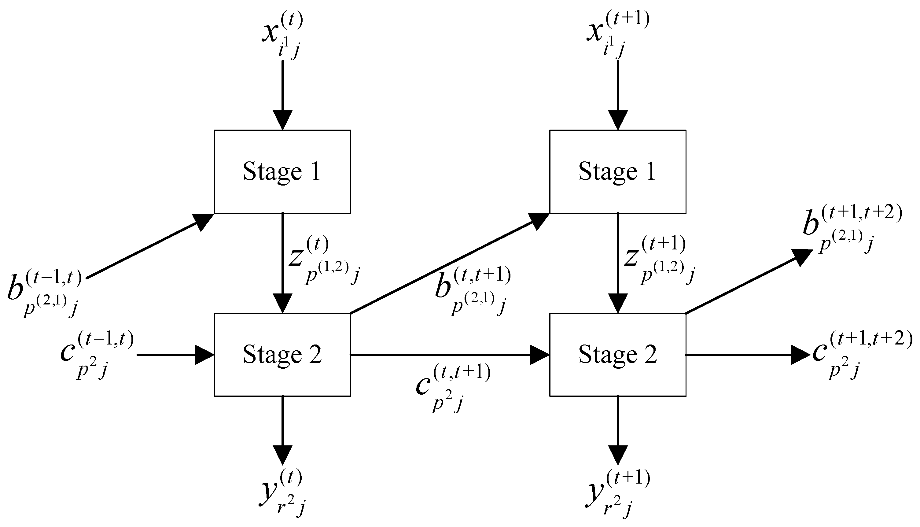
2.1. Nomenclatures and Dynamic Network Structure

Consider $N$ DMUs (banks) in period $t(t=1,2,\cdots ,T)$ and assume that the production process of the bank can be divided into two stages—the deposit and loan stages—also known as the productivity and profitability stages, respectively. We define the intensity variable column for the first stage as ${\mathsf{\lambda }}^{(t)}=({\lambda }_1^{(t)},{\lambda }_2^{(t)},\cdots ,{\lambda }_N^{(t)})\in {ℝ}_{+}^N$ and for the second stage the intensity column vector is ${\mathsf{\gamma }}^{(t)}=({\gamma }_1^{(t)},{\gamma }_2^{(t)},\cdots ,{\gamma }_N^{(t)})\in {ℝ}_{+}^N$. Assuming that there are $H(H>1)$ technology-heterogeneous groups and $N_h$ DMUs in group $h$, where for each period we have ${\displaystyle \sum _{h=1}^H{N}_h=N}$. As shown in Figure 1, let $x_{i^{1}j}^{(t)}$, $i^1=1,2,\cdots ,m^1$, denote the original input to the deposit stage in period $t$. In the deposit stage, each bank produces intermediate products $z_{p^{(1,2)}j}^{(t)}(p^{(1,2)}=1,2,\cdots ,q^{(1,2)})$ by using the original input $x_{i^{1}j}^{(t)}$ in period $t$. The undesirable outputs produced in a previous period have the effect of reducing the subsequent period’s production possibilities since non-performing loans require the bank to raise more equity capital or reduce their production of deposits. Similarly, we used non-performing loans as undesirable carryovers. The undesirable output from period $t-1$ is $b_{p^{(2,1)}j}^{(t-1,t)}(p^{(2,1)}=1,2,\cdots ,q^{(2,1)})$, where $b_{p^{(2,1)}j}^{(t-1,t)}$ are undesirable carryovers from the preceding (current) period to the current (subsequent) period and superscripts $(1,2)$ and $(2,1)$ indicate that these indicators are from the deposit (loan) stage to the loan (deposit) stage, respectively. In the loan stage, each bank in period $t$ uses intermediate products $z_{p^{(1,2)}j}^{(t)}$ obtained from the deposit stage and $c_{p^{2}j}^{(t-1,t)}(p^2=1,2,\cdots ,q^2)$ to produce output $y_{r^{2}j}^{(t)}(r^2=1,2,\cdots ,s^2)$, $c_{p^{2}j}^{(t,t+1)}$ and $b_{p^{(2,1)}j}^{(t,t+1)}$, where $c_{p^{2}j}^{(t,t+1)}$ and $b_{p^{(2,1)}j}^{(t,t+1)}$ are desirable and undesirable carryovers from the current period to the subsequent period, respectively. All the variables are strictly greater than zero.

2.2. Graphical Explanations

For demonstration purposes, we consider two technologies or group frontiers—I and II—labelled in Figure 1 as “GHDEF” and “BCJKL,” respectively. The convex metafrontier (BCDEF) and non-convex metafrontier (BCIDEF) are enveloped by these two group frontiers. As seen in Figure 2, the convex metafrontier includes the “Infeasible Input-Output combinations,” which is the grey-shaded area labelled as “CID.” For example, let’s take the inefficient DMU $A_0$. Its input-oriented and output-oriented efficiency values with reference to group frontiers are, respectively estimated as follows:

$$\mathrm{Technology} \mathrm{I}: E_i^{\mathrm{I}}=\frac{A_0{A}_4-A_0{A}_1}{A_0{A}_4}; E_o^{\mathrm{I}}=\frac{A_0{A}_8}{A_0{A}_8+A_0{A}_6}$$

$$\mathrm{Technology} \mathrm{II}: E_i^{\mathrm{II}}=\frac{A_0{A}_4-A_0{A}_2}{A_0{A}_4}; E_o^{\mathrm{II}}=\frac{A_0{A}_8}{A_0{A}_8+A_0{A}_5}$$

where $i$ and $o$ denote input-oriented and output-oriented.

Obviously, efficiency scores of group frontiers are identified with reference to the convex or non-convex metafrontier; the main differences are the DMU efficiency scores on the convex or non-convex metafrontier. The input- and output-oriented efficiency values with reference to the convex and non-convex metafrontiers are, respectively, estimated as follows:

$$\mathrm{Convex} \mathrm{metafrontier}: E_i^{\mathrm{c}-\mathrm{meta}}=\frac{A_0{A}_4-A_0{A}_3}{A_0{A}_4}; E_o^{\mathrm{c}-\mathrm{meta}}=\frac{A_0{A}_8}{A_0{A}_8+A_0{A}_7}$$

$$\mathrm{Non}-\mathrm{convex} \mathrm{metafrontier}: E_i^{\mathrm{nc}-\mathrm{meta}}=\frac{A_0{A}_4-A_0{A}_2}{A_0{A}_4}; E_o^{\mathrm{nc}-\mathrm{meta}}=\frac{A_0{A}_8}{A_0{A}_8+A_0{A}_6}$$

It is obvious to obtain that $E_i^{\mathrm{nc}-\mathrm{meta}}\ge E_i^{\mathrm{c}-\mathrm{meta}}$ since $A_0{A}_2\le A_0{A}_3$ and $E_i^{\mathrm{nc}-\mathrm{meta}}=E_i^{\mathrm{c}-\mathrm{meta}}$ if and only if $A_0{A}_2=A_0{A}_3$. And the same for $E_o^{\mathrm{nc}-\mathrm{meta}}\ge E_o^{\mathrm{c}-\mathrm{meta}}$ since $A_0{A}_6\le A_0{A}_7$, $E_o^{\mathrm{nc}-\mathrm{meta}}=E_o^{\mathrm{c}-\mathrm{meta}}$ if and only if $A_0{A}_6=A_0{A}_7$. Integrating input-oriented and output-oriented becomes the non-oriented estimations. In sum, some DMU efficiency scores may be underestimated if we do not take the non-convex metafrontier and slacks into account, leading to bias estimations of in both the efficiency measurement and empirical test.

2.3. Non-Convex Metafrontier Slacks-Based Bank Super-Efficiency

The radial efficiency measure and the non-radial efficiency measure are the two measures commonly used to evaluate DMU efficiency. The shortcoming of the former approach is that it neglects non-radial input/output slacks; that is, it cannot provide detailed information regarding the inefficiency of a specific input/output. The SBM as a non-radial measure can directly deal with the “input excess” and “output shortfall” problems, where the objective function value can be interpreted as the ratio of mean input and output mix of inefficiencies. Approaches using slacks-based measures can effectively explore the sources of inefficiency behind the operational processes of each bank from this point of view. In this subsection, we mainly focus on the proposed NCMeta-US-DNSBM model, which simultaneously incorporates the non-convex metafrontier technique, undesirable outputs and super-efficiency into the dynamic network SBM model. Due to the lack of space, the production possibility sets are provided in Appendix A.

To obtain a more comprehensive and reasonable estimate of bank efficiency, especially for stages of efficiency, it is necessary to extend the convex frontier to a non-convex one in a dynamic network SBM model that can be programmed as Formula (1).

$$\begin{array}{l}{\rho }_{ko}^{nc-meta\ast }=\min \frac{{\displaystyle \sum _{t=1}^T{\omega }^{(t)}\left\{{\beta }_1\left[1+\frac{1}{m^1+q^{(2,1)}}\left({\displaystyle \sum _{i^1=1}^{m^1}\frac{s_{i^{1}ko}^{(t)-}}{x_{i^{1}ko}^{(t)}}}+{\displaystyle \sum _{p^{(2,1)}=1}^{q^{(2,1)}}\frac{s_{p^{(2,1)}ko}^{(t-1,t)-}}{b_{p^{(2,1)}ko}^{(t-1,t)}}}\right)\right]+{\beta }_2\left[1+\left(\frac{1}{q^2}{\displaystyle \sum _{p^2=1}^{q^2}\frac{s_{p^{2}ko}^{(t-1,t)-}}{c_{p^{2}ko}^{(t-1,t)}}+\frac{1}{q^{(1,2)}}{\displaystyle \sum _{p^{(1,2)}=1}^{q^{(1,2)}}\frac{s_{p^{(1,2)}ko}^{(t)-}}{z_{p^{(1,2)}ko}^{(t)}}}}\right)\right]\right\}}}{{\displaystyle \sum _{t=1}^T{\omega }^{(t)}}\left\{{\beta }_1\left(1-\frac{1}{q^{(1,2)}}{\displaystyle \sum _{p^{(1,2)}=1}^{q^{(1,2)}}\frac{s_{p^{(1,2)}ko}^{(t)+}}{z_{p^{(1,2)}ko}^{(t)}}}\right)+{\beta }_2\left[1-\left(\frac{1}{s^2}{\displaystyle \sum _{r^2=1}^{s^2}\frac{s_{r^{2}ko}^{(t)+}}{y_{r^{2}ko}^{(t)}}+\frac{1}{q^2}{\displaystyle \sum _{p^2=1}^{q^2}\frac{s_{p^{2}ko}^{(t,t+1)+}}{c_{p^{2}ko}^{(t,t+1)}}}}+\frac{1}{q^{(2,1)}}{\displaystyle \sum _{p^{(2,1)}=1}^{q^{(2,1)}}\frac{s_{p^{(2,1)}ko}^{(t,t+1)+}}{b_{p^{(2,1)}ko}^{(t,t+1)}}}\right)\right]\right\}}\\ s.t. x_{i^{1}ko}^{(t)}-{\displaystyle {\sum }_{h=1}^H{\displaystyle {\sum }_{j=1,j\ne o if h=k}^{N_k}{\lambda }_{hj}^{(t)}{x}_{i^{1}hj}^{(t)}-s_{i^{1}ko}^{(t)-}=0,}} \forall i^1,\forall t;\\ \hspace{1em}\hspace{1em}{b}_{p^{(2,1)}ko}^{(t-1,t)}-{\displaystyle {\sum }_{h=1}^H{\displaystyle {\sum }_{j=1,j\ne o if h=k}^{N_k}{\lambda }_{hj}^{(t)}{b}_{p^{(2,1)}hj}^{(t-1,t)}}}-s_{p^{(2,1)}ko}^{(t-1,t)-}=0,\forall p^{(2,1)},\forall t;\\ \hspace{1em}{c}_{p^{2}ko}^{(t-1,t)}-{\displaystyle {\sum }_{h=1}^H{\displaystyle {\sum }_{j=1,j\ne o if h=k}^{N_k}{\gamma }_{hj}^{(t)}{c}_{p^{2}hj}^{(t-1,t)}}}-s_{p^{2}ko}^{(t-1,t)-}=0,\forall p^2,\forall t;\\ \hspace{1em}\hspace{1em}{z}_{p^{(1,2)}ko}^{(t)}-{\displaystyle {\sum }_{h=1}^H{\displaystyle {\sum }_{j=1,j\ne o if h=k}^{N_k}{\gamma }_{hj}^{(t)}{z}_{p^{(1,2)}hj}^{(t)}}}-s_{p^{(1,2)}ko}^{(t)-}=0, \forall p^{(1,2)},\forall t;\\ \hspace{1em}\hspace{1em}{\displaystyle {\sum }_{h=1}^H{\displaystyle {\sum }_{j=1,j\ne o if h=k}^{N_k}{\lambda }_{hj}^{(t)}{z}_{p^{(1,2)}hj}^{(t)}}}={\displaystyle {\sum }_{h=1}^H{\displaystyle {\sum }_{j=1,j\ne o if h=k}^{N_k}{\gamma }_{hj}^{(t)}{z}_{p^{(1,2)}hj}^{(t)}}},\forall p^{(1,2)},\forall t;\\ \hspace{1em}\hspace{1em}{\displaystyle {\sum }_{h=1}^H{\displaystyle {\sum }_{j=1,j\ne o if h=k}^{N_k}{\lambda }_{hj}^{(t)}{z}_{p^{(1,2)}hj}^{(t)}}}-z_{p^{(1,2)}ko}^{(t)}-s_{p^{(1,2)}ko}^{(t)+}=0, \forall p^{(1,2)},\forall t;\\ \hspace{1em}\hspace{1em}{\displaystyle {\sum }_{h=1}^H{\displaystyle {\sum }_{j=1,j\ne o if h=k}^{N_k}{\gamma }_{hj}^{(t)}{y}_{r^{2}hj}^{(t)}}}-y_{r^{2}ko}^{(t)}-s_{r^{2}ko}^{(t)+}=0, \forall r^2,\forall t;\\ \hspace{1em}\hspace{1em}{\displaystyle {\sum }_{h=1}^H{\displaystyle {\sum }_{j=1,j\ne o if h=k}^{N_k}{\gamma }_{hj}^{(t)}{c}_{p^{2}hj}^{(t,t+1)}}}-c_{p^{2}ko}^{(t,t+1)}-s_{p^{2}ko}^{(t,t+1)+}=0,\forall p^2,\forall t;\\ \hspace{1em}\hspace{1em}{b}_{p^{(2,1)}ko}^{(t,t+1)}-{\displaystyle {\sum }_{h=1}^H{\displaystyle {\sum }_{j=1,j\ne o if h=k}^{N_k}{\gamma }_{hj}^{(t)}{b}_{p^{(2,1)}hj}^{(t,t+1)}}}-s_{p^{(2,1)}ko}^{(t,t+1)+}=0,\forall p^{(2,1)},\forall t;\\ \hspace{1em}\hspace{1em}{\displaystyle {\sum }_{h=1}^H{\displaystyle {\sum }_{j=1,j\ne o if h=k}^{N_k}{\gamma }_{hj}^{(t)}{c}_{p^{2}hj}^{(t-1,t)}}}={\displaystyle {\sum }_{h=1}^H{\displaystyle {\sum }_{j=1,j\ne o if h=k}^{N_k}{\gamma }_{hj}^{(t)}{c}_{p^{2}hj}^{(t,t+1)}}},\forall p^2,\forall t;\\ \hspace{1em}\hspace{1em}{\beta }_1\left(1-\frac{1}{q^{(1,2)}}{\displaystyle \sum _{p^{(1,2)}=1}^{q^{(1,2)}}\frac{s_{p^{(1,2)}ko}^{(t)+}}{z_{p^{(1,2)}ko}^{(t)}}}\right)+{\beta }_2\left[1-\left(\frac{1}{s^2}{\displaystyle \sum _{r^2=1}^{s^2}\frac{s_{r^{2}ko}^{(t)+}}{y_{r^{2}ko}^{(t)}}+\frac{1}{q^2}{\displaystyle \sum _{p^2=1}^{q^2}\frac{s_{p^{2}ko}^{(t,t+1)+}}{c_{p^{2}ko}^{(t,t+1)}}}}+\frac{1}{q^{(2,1)}}{\displaystyle \sum _{p^{(2,1)}=1}^{q^{(2,1)}}\frac{s_{p^{(2,1)}ko}^{(t,t+1)+}}{b_{p^{(2,1)}ko}^{(t,t+1)}}}\right)\right]\ge \epsilon ;\\ \hspace{1em}\hspace{1em}{\displaystyle {\sum }_{h=1}^H{\displaystyle {\sum }_{j\in (k=1),j\ne o if h=k}^{N_k}{\lambda }_{hj}^{(t)}}}={\eta }_1,{\displaystyle {\sum }_{h=1}^H{\displaystyle {\sum }_{j\in (k=2),j\ne o if h=k}^{N_k}{\lambda }_{hj}^{(t)}}}={\eta }_2,\cdots ,{\displaystyle {\sum }_{h=1}^H{\displaystyle {\sum }_{j\in (k=H),j\ne o if h=k}^{N_k}{\lambda }_{hj}^{(t)}}}={\eta }_H;\\ \hspace{1em}\hspace{1em}{\displaystyle {\sum }_{h=1}^H{\displaystyle {\sum }_{j\in (k=1),j\ne o if h=k}^{N_k}{\gamma }_{hj}^{(t)}}}={\mu }_1,{\displaystyle {\sum }_{h=1}^H{\displaystyle {\sum }_{j\in (k=2),j\ne o if h=k}^{N_k}{\gamma }_{hj}^{(t)}}}={\mu }_2,\cdots ,{\displaystyle {\sum }_{h=1}^H{\displaystyle {\sum }_{j\in (k=H),j\ne o if h=k}^{N_k}{\gamma }_{hj}^{(t)}}}={\mu }_H;\\ \hspace{1em}\hspace{1em}{\displaystyle {\sum }_{h=1}^H{\eta }_h}=1; {\displaystyle {\sum }_{h=1}^H{\mu }_h}=1;{\eta }_h=1 \mathrm{or} 0; {\mu }_h=1 \mathrm{or} 0;\\ \hspace{1em}\hspace{1em}{s}_{i^{1}ko}^{(t)-},s_{p^{(2,1)}ko}^{(t-1,t)-},s_{p^{2}ko}^{(t-1,t)-},s_{p^{(1,2)}ko}^{(t)-},s_{p^{(1,2)}ko}^{(t)+},s_{r^{2}ko}^{(t)+},s_{p^{2}ko}^{(t,t+1)+},s_{p^{(2,1)}ko}^{(t,t+1)+},{\lambda }_{hj}^{(t)},{\gamma }_{hj}^{(t)}\ge 0;\\ \hspace{1em}\hspace{1em}t=1,2,\cdots ,T; j=1,2,\cdots ,N_k; k,h=1,2,\cdots ,H.\end{array}$$

(1)

where ${\displaystyle \sum _{t=1}^T{\omega }^{(t)}}=1$, ${\beta }_1+{\beta }_2=1$. When comparing the importance of each time period, it would be reasonable that the last period T has the top priority and the largest contribution to the system and those pertaining to T − 1, T − 2, …, T − 1 decrease in this order [19]. As such, the weights attached to years 2010, 2011, 2012, 2013 and 2014 are assumed to be ω⁽¹⁾ = 0.1, ω⁽²⁾ = 0.15, ω⁽³⁾ = 0.2, ω⁽⁴⁾ = 0.25, ω⁽⁵⁾ = 0.3, respectively. Supposing that two stages are equally important, then β₁ = β₂ = 0.5. $\lambda$ and $\gamma$ are non-negative weights in the deposit stage and loan stage, respectively, and $s$ represents the slacks. The term $\epsilon$ is a non-Archimedean value and the corresponding constraint ensuring the denominator in the objective function is greater than zero.

The fractional program of Formula (1) can be transformed into a linear programming problem using the Charnes-Cooper transformation [40]. A linear programming approach to efficiency evaluation in non-convex meta-technologies is proposed in Reference [41]. Thus, it is possible to compute bank efficiency considering the non-convex metafrontier. Since the optimal objective values are ${\rho }_{ko}^{group\ast }$ and ${\rho }_{ko}^{nc-meta\ast }$, we can then compute the technology gap ratio (TGR), which is alternatively defined as a meta-technology ratio in the literature, which enables a greater understanding of the bank efficiency improvement potential and measures the technology gap between the group frontier and non-convex metafrontier technologies.

$$TG{R}_{ko}^{nc}=\frac{{\rho }_{ko}^{nc-meta\ast }}{{\rho }_{ko}^{group\ast }}$$

(2)

Since the non-convex metafrontier is enveloped by the specific group frontier and excludes the area labeled “Infeasible Input-Output combinations,” along with ${\rho }_{ko}^{nc-meta\ast }\le {\rho }_{ko}^{group\ast }$, ensuring that $TG{R}_{ko}^{nc}$ ranges from zero to one, a higher TGR indicates that the group frontier technology is closer to the non-convex metafrontier technology.

Unless otherwise mentioned, the efficiency scores presented in this paper are estimated with reference to the non-convex metafrontier. Given that, the period efficiency can be formally stated as:

$${\rho }_{ko}^{(t)\ast }=\frac{{\beta }_1\left[1+\frac{1}{m^1+q^{(2,1)}}\left({\displaystyle \sum _{i^1=1}^{m^1}\frac{s_{i^{1}ko}^{(t)-}}{x_{i^{1}ko}^{(t)}}}+{\displaystyle \sum _{p^{(2,1)}=1}^{q^{(2,1)}}\frac{s_{p^{(2,1)}ko}^{(t-1,t)-}}{b_{p^{(2,1)}ko}^{(t-1,t)}}}\right)\right]+{\beta }_2\left[1+\left(\frac{1}{q^2}{\displaystyle \sum _{p^2=1}^{q^2}\frac{s_{p^{2}ko}^{(t-1,t)-}}{c_{p^{2}ko}^{(t-1,t)}}+\frac{1}{q^{(1,2)}}{\displaystyle \sum _{p^{(1,2)}=1}^{q^{(1,2)}}\frac{s_{p^{(1,2)}ko}^{(t)-}}{z_{p^{(1,2)}ko}^{(t)}}}}\right)\right]}{{\beta }_1\left(1-\frac{1}{q^{(1,2)}}{\displaystyle \sum _{p^{(1,2)}=1}^{q^{(1,2)}}\frac{s_{p^{(1,2)}ko}^{(t)+}}{z_{p^{(1,2)}ko}^{(t)}}}\right)+{\beta }_2\left[1-\left(\frac{1}{s^2}{\displaystyle \sum _{r^2=1}^{s^2}\frac{s_{r^{2}ko}^{(t)+}}{y_{r^{2}ko}^{(t)}}+\frac{1}{q^2}{\displaystyle \sum _{p^2=1}^{q^2}\frac{s_{p^{2}ko}^{(t,t+1)+}}{c_{p^{2}ko}^{(t,t+1)}}}}+\frac{1}{q^{(2,1)}}{\displaystyle \sum _{p^{(2,1)}=1}^{q^{(2,1)}}\frac{s_{p^{(2,1)}ko}^{(t,t+1)+}}{b_{p^{(2,1)}ko}^{(t,t+1)}}}\right)\right]}$$

(3)

The deposit stage efficiency and loan stage efficiency under the $k^{th}(k=1,2,\cdots ,H)$ group frontier over multi-periods can be represented as ${\rho }_{ko1}^{\ast }$ and ${\rho }_{ko2}^{\ast }$, respectively, as follows:

$${\rho }_{ko1}^{\ast }=\frac{{\displaystyle \sum _{t=1}^T{\omega }^{(t)}\left[1+\frac{1}{m^1+q^{(2,1)}}\left({\displaystyle \sum _{i^1=1}^{m^1}\frac{s_{i^{1}ko}^{(t)-}}{x_{i^{1}ko}^{(t)}}}+{\displaystyle \sum _{p^{(2,1)}=1}^{q^{(2,1)}}\frac{s_{p^{(2,1)}ko}^{(t-1,t)-}}{b_{p^{(2,1)}ko}^{(t-1,t)}}}\right)\right]}}{{\displaystyle \sum _{t=1}^T{\omega }^{(t)}}\left(1-\frac{1}{q^{(1,2)}}{\displaystyle \sum _{p^{(1,2)}=1}^{q^{(1,2)}}\frac{s_{p^{(1,2)}ko}^{(t)+}}{z_{p^{(1,2)}ko}^{(t)}}}\right)},$$

(4)

$${\rho }_{ko2}^{\ast }=\frac{{\displaystyle \sum _{t=1}^T{\omega }^{(t)}\left[1+\left(\frac{1}{q^2}{\displaystyle \sum _{p^2=1}^{q^2}\frac{s_{p^{2}ko}^{(t-1,t)-}}{c_{p^{2}ko}^{(t-1,t)}}+\frac{1}{q^{(1,2)}}{\displaystyle \sum _{p^{(1,2)}=1}^{q^{(1,2)}}\frac{s_{p^{(1,2)}ko}^{(t)-}}{z_{p^{(1,2)}ko}^{(t)}}}}\right)\right]}}{{\displaystyle \sum _{t=1}^T{\omega }^{(t)}}\left[1-\left(\frac{1}{s^2}{\displaystyle \sum _{r^2=1}^{s^2}\frac{s_{r^{2}ko}^{(t)+}}{y_{r^{2}ko}^{(t)}}+\frac{1}{q^2}{\displaystyle \sum _{p^2=1}^{q^2}\frac{s_{p^{2}ko}^{(t,t+1)+}}{c_{p^{2}ko}^{(t,t+1)}}}}+\frac{1}{q^{(2,1)}}{\displaystyle \sum _{p^{(2,1)}=1}^{q^{(2,1)}}\frac{s_{p^{(2,1)}ko}^{(t,t+1)+}}{b_{p^{(2,1)}ko}^{(t,t+1)}}}\right)\right]}.$$

(5)

In this case, the period stage efficiencies of these two stages are defined as ${\rho }_{ko1}^{(t)\ast }$ and ${\rho }_{ko2}^{(t)\ast }$, respectively, as follows:

$${\rho }_{ko1}^{(t)\ast }=\frac{1+\frac{1}{m^1+q^{(2,1)}}\left({\displaystyle \sum _{i^1=1}^{m^1}\frac{s_{i^{1}ko}^{(t)-}}{x_{i^{1}ko}^{(t)}}}+{\displaystyle \sum _{p^{(2,1)}=1}^{q^{(2,1)}}\frac{s_{p^{(2,1)}ko}^{(t-1,t)-}}{b_{p^{(2,1)}ko}^{(t-1,t)}}}\right)}{1-\frac{1}{q^{(1,2)}}{\displaystyle \sum _{p^{(1,2)}=1}^{q^{(1,2)}}\frac{s_{p^{(1,2)}ko}^{(t)+}}{z_{p^{(1,2)}ko}^{(t)}}}},$$

(6)

$${\rho }_{ko2}^{(t)\ast }=\frac{1+\left(\frac{1}{q^2}{\displaystyle \sum _{p^2=1}^{q^2}\frac{s_{p^{2}ko}^{(t-1,t)-}}{c_{p^{2}ko}^{(t-1,t)}}+\frac{1}{q^{(1,2)}}{\displaystyle \sum _{p^{(1,2)}=1}^{q^{(1,2)}}\frac{s_{p^{(1,2)}ko}^{(t)-}}{z_{p^{(1,2)}ko}^{(t)}}}}\right)}{1-\left(\frac{1}{s^2}{\displaystyle \sum _{r^2=1}^{s^2}\frac{s_{r^{2}ko}^{(t)+}}{y_{r^{2}ko}^{(t)}}+\frac{1}{q^2}{\displaystyle \sum _{p^2=1}^{q^2}\frac{s_{p^{2}ko}^{(t,t+1)+}}{c_{p^{2}ko}^{(t,t+1)}}}}+\frac{1}{q^{(2,1)}}{\displaystyle \sum _{p^{(2,1)}=1}^{q^{(2,1)}}\frac{s_{p^{(2,1)}ko}^{(t,t+1)+}}{b_{p^{(2,1)}ko}^{(t,t+1)}}}\right)}.$$

(7)

3. Data

The datasets used in this paper include 36 commercial banks in mainland China taken from the Bureau van Dijk (Bankscope) for the period 2009–2014. In dynamic network structure settings, the period should be included 2009, as the carryovers (NPLs from the deposit stage to the loan stage and other earning assets in the loan stage) in 2009 are treated as inputs in 2010. In addition, due to the availability of data, macroeconomic (environmental) variables, such as the GDP (Gross Domestic Product) growth rate, GDP deflator and growth of M2 (money and quasi-money), were obtained from the World Bank Group. We use three inputs: fixed assets (fixed_asset), equity (equity) and personnel expenses (personnel_expenses). The deposits (deposits) are treated as intermediates in the two-stage network DEA framework. The desirable and undesirable carryovers are other earning assets (other_earning_assets) and non-performing loans (NPLs), respectively. The final output of the loan stage is gross loans (gross_loans). The number of NPLs, which expanded in the aftermath of the 1997 Asian financial crisis, has declined in most Southeast Asian countries since 2009. Few previous studies analyzed the factors that contributed to the reduction in Asia [42]. Moreover, data on off-balance sheet (OBS) items are not available, especially in 2009 and 2010, so for now, we do not consider OBS items as one of the outputs, though they will mostly capture the non-traditional activities that banks are engaged in. All financial data are deflated by the GDP deflator (base year = 2009). The descriptive statistics of all inputs, intermediates, carryovers and outputs used in our analytical framework are summarized in

Table 1. Descriptive statistics of input-output variables (Unit: ten thousand USD).

	Obs.	Mean	Std. Dev.	Min.	Max.	95% Confidence Interval
						Lower	Upper
	Panel A: Total banks
Original inputs
fixed_asset	216	218.09	500.98	0.07	2003.27	151.28	284.90
equity	216	1308.36	2735.72	15.56	12,146.59	943.53	1673.20
personnel_expenses	216	128.78	267.82	0.56	1082.21	93.06	164.49
Intermediate
deposits	216	22,128.80	45,116.27	58.73	193,406.20	16,112.15	28,145.44
Final outputs
gross_loans	216	12,580.90	24,831.09	52.90	102,489.00	9269.46	15,892.34
other_earn_assets	216	11,309.88	24,049.12	20.78	105,917.70	8102.73	14,517.04
npls	216	303.06	644.92	0.56	2602.24	217.05	389.07
	Panel B: SOBs
Original inputs
fixed_asset	24	1586.73	265.79	1093.89	2003.27	1480.40	1693.07
equity	24	8600.03	2069.33	5022.19	12,146.59	7772.14	9427.92
personnel_expenses	24	860.97	106.68	665.97	1082.21	818.29	903.65
Intermediate
deposits	24	144,080.00	21,255.05	113,865.60	193,406.20	135,576.40	152,583.60
Final outputs
gross_loans	24	79,262.75	10,578.89	60,604.36	102,489.00	75,030.40	83,495.11
other_earn_assets	24	76,304.48	14,421.35	52,742.49	105,917.70	70,534.85	82,074.12
npls	24	2070.54	231.12	1654.17	2602.24	1978.07	2163.00
	Panel C: JSBs
Original inputs
fixed_asset	114	77.95	114.88	1.96	534.54	56.86	99.04
equity	114	617.15	736.29	31.62	2941.68	481.99	752.31
personnel_expenses	114	58.93	69.77	2.11	226.96	46.12	71.73
Intermediate
deposits	114	11,181.78	13,461.54	389.81	54,123.37	8710.68	13,652.88
Final outputs
gross_loans	114	6895.02	8393.22	283.63	32,906.58	5354.30	8435.74
other_earn_assets	114	5182.33	6225.30	64.97	25,478.56	4039.57	6325.09
npls	114	135.78	164.02	2.31	675.84	105.67	165.89
	Panel D: FBs
Original inputs
fixed_asset	78	1.79	1.97	0.07	8.84	1.36	2.23
equity	78	75.01	48.80	15.56	219.24	64.18	85.84
personnel_expenses	78	5.58	6.09	0.56	25.63	4.23	6.93
Intermediate
deposits	78	604.84	644.61	58.73	2489.99	461.79	747.90
Final outputs
gross_loans	78	373.55	293.28	52.90	1170.96	308.46	438.63
other_earn_assets	78	267.21	357.62	20.78	1302.72	187.84	346.57
npls	78	3.70	2.53	0.56	10.94	3.14	4.27

Note: SOBs, JSBs and FBs represent state-owned banks, joint-stock banks and foreign banks, respectively.

, indicating that significant differences among banks exist. Input-output variables of state-owned banks (joint-stock banks) are much higher than joint-stock banks (foreign banks) and fixed_asset, thus state-owned banks (joint-stock banks) produce more NPLs during the production process.

4. Empirical Analysis and Econometric Strategy

4.1. Measurement Of Bank Efficiency

Following [43], we assume variable returns to scale (VRS) in models (1) and (3)–(7). Different types of banks perform differently due to technological heterogeneity, which is reflected in varying efficiency scores. We provide the in-depth analysis for why the non-convex metafrontier is more appropriate than the convex metafrontier for measuring bank efficiency in a dynamic network framework. In addition to the graphical evidence (see Figure 2), we also used the bank efficiency measured by the convex metafrontier method (details are provided in Appendix B) for comparison, as shown in

Table 2. Comparative analysis of bank efficiency for different stages and frontiers.

	(1) Banks	(2) Years	(3) Convex	(4) Non-Convex	(5) Group	(6) TGR c	(7) TGR nc
Panel A: Deposit Stage
Vertical comparison 1	B12 [2]	2010	1.0970	1.0912	1.0912	1.0053	1.0000
	B12 [2]	2011	0.9774	0.9736	0.9736	1.0039	1.0000
Vertical comparison 2	B28 [1]	2013	1.0000	0.9323	0.9323	1.0726	1.0000
	B28 [1]	2014	1.0000	0.9324	0.9324	1.0725	1.0000
Horizontal comparison	B9 [1]	2014	0.9966	0.9953	0.9953	1.0013	1.0000
	B15 [1]	2014	1.2272	1.0837	1.0837	1.1324	1.0000
Panel B: Loan Stage
Vertical comparison 1	B6 [3]	2010	1.2063	1.1977	1.1977	1.0072	1.0000
	B6 [3]	2012	0.7231	0.7207	0.7207	1.0033	1.0000
Vertical comparison 2	B30 [2]	2013	0.9912	0.9463	0.9463	1.0475	1.0000
	B30 [2]	2014	0.9388	0.8985	0.8985	1.0448	1.0000
Horizontal comparison	B21 [3]	2013	1.2219	1.0000	1.0000	1.2219	1.0000
	B36 [2]	2013	0.9945	0.9467	0.9467	1.0505	1.0000

Notes: (1) TGR denotes the technology gap ratio, superscripts c and nc represent convex and non-convex, respectively; (2) (6) = (3)/(5), (7) = (4)/(5); (3) Numbers in square brackets identify heterogeneous groups, ‘1,’ ‘2’ and ‘3’ represent state-owned banks, joint-stock banks and foreign banks, respectively; (4) B12, B28, B9, B15, B6, B30, B21, B36 stand for China Guangfa Bank Co Ltd., Bank of China Limited, Shanghai Pudong Development Bank, Agricultural Bank of China Limited, Credit Agricole CIB (China), Hua Xia Bank Co Limited, DBS BANK (China) Limited and Bank of Beijing Co Ltd., respectively. The list of 36 Chinese commercial banks is provided in Appendix C.

. Evidently, bank efficiency scores obtained from different groups with reference to the convex and non-convex metafrontier are the same (Column (5)). However, the technology gap ratio (TGR) may greater than unity when measuring stage efficiencies for some DMUs. As seen in Table 2, compared to the efficiency scores measured by the non-convex metafrontier (Column (4)), bank efficiency scores in both the deposit and loan stages are overestimated with reference to the convex metafrontier (Column (3)). The findings also indicate that the non-convex metafrontier is more reasonable for measuring bank efficiency, especially in a dynamic network case. Thus, we discuss bank efficiency measured by the proposed NCMeta-US-DNSBM model in the following context.

As visually illustrated in Figure 3, the SOB efficiency scores measured by the proposed model are generally the highest and the lowest for the FB, whether on different frontiers or in different stages. Furthermore, the FB deposit stage efficiency and the JSB loan stage efficiency are lower than the total bank efficiency scores on average. Thus, for different bank types, the development of bank efficiency is unbalanced and most banks have much room for improvement. Figure 3 additionally shows the TGRs of different banks, indicating that the group frontier technology of SOB TGRs is closer to the non-convex metafrontier technology compared to those of JSB and FB. The findings are consistent with Reference [44] who concluded that SOBs are more efficient than JSBs by using the directional distance function and the metafrontier-Luenberger productivity indicator. However, this contradicts the results of Reference [13]. Consequently, non-convex metafrontier analysis, super efficiency and dynamic network structure all should be considered in the production processes of the banking industry and the efficiency scores computed by the proposed model in this study are more beneficial to commercial bank policy-makers and managers. Are the efficiency gaps between different groups statistically significant? To shed light on the significance of the difference between SOBs, JSBs and FBs, we performed a Kolmogorov-Smirnov test for bank efficiency. The comparison is presented in

Table 3. The comparison of different sub-efficiencies of different groups.

Groups	Kolmogorov-Smirnov Test	t-Test (t-Value)	Sign Rank Test (Z-Value)
Period Efficiency
SOB versus JSB	0.7474 ***	4.2095 ***	4.7980 ***
SOB versus FB	0.7538 ***	4.4947 ***	4.7670 ***
JSB versus FB	0.3401 ***	2.450 8**	2.9730 ***
Deposit Stage Efficiency
SOB versus JSB	0.4763 ***	2.9059 ***	2.8500 ***
SOB versus FB	0.5692 ***	1.2918	2.9650 ***
JSB versus FB	0.3117 ***	0.2019	2.2380 **
Loan Stage Efficiency
SOB versus JSB	0.5368 ***	2.4636 **	2.7690 ***
SOB versus FB	0.5385 ***	2.4295 **	1.9010 *
JSB versus FB	0.2162 ***	1.2427	0.9280

Note: ***, ** and * denote significance at the levels of 1%, 5% and 10%, respectively.

. As shown in Table 3, we can reject the null hypothesis that bank efficiencies are identical for SOBs, JSBs and FBs. Moreover, both the t-test and the sign rank test also reveal that there are significance differences among the three groups in different stages. Thus, it is necessary to consider heterogeneity while measuring bank efficiency.

The time evolution of period efficiency, deposit stage efficiency and loan stage efficiency in Figure 4 shows a process of ongoing and quite significant convergence. As seen in the graph, kernel density estimation curves of period efficiency and deposit stage efficiency are moving to the right every year but shifting to the left for loan stage efficiency. The period efficiency scores are mainly distributed in [0.2, 2.0] in 2010 and have a tall structure in 2012, ranging from [0.3, 1.3]. The have a flat structure in 2014, ranging from [0.3, 2.0] and have two peaks located at approximately 0.5 and 1.0. Also, the distribution layout of deposit stage efficiency is fairly similar to that of period efficiency, both of which have a cluster of high efficiency values, though the peak located at approximately 1.0 is significantly higher compared to period efficiency. The kernel density estimation of efficiency scores becomes cliffy and moves from right in 2010 to left in 2014, in terms of loan stage. Also, the peak of approximately 1.0 is significantly higher than the deposit stage peak. Thus, as time goes on, the disparity of kernel density estimations for these efficiency scores has declined. In summary, the kernel density estimations provide evidence that the period efficiency of commercial banks in China improved gradually from 2010–2014.

Furthermore, we also adopted the non-parametric estimation of conditional kernel density to examine the stability and liquidity of bank efficiency distribution for a more accurate, visual perspective [45]. Specifically, we provide the stacked conditional density (SCD) and highest density regions (HDR) plots of bank efficiency; these plots visually illustrate the conditional densities, as seen in Figure 5. Regarding period efficiency (Figure 5a,b), the ridges of the SCD plots that deviate from the 45-degree diagonal line indicate that the efficiency of the period exhibits significant internal liquidity. The black dots of the HDR plots represent the conditional values with different conditions, while the conditional values correspond equally to the peaks of the SCD plots, which are the maximums of the conditional densities. Each rectangle represents the conditional density of period bank efficiency at year t, from shallow to deep, respectively and represent 25% HDR, 50% HDR and 90% HDR. As seen in Figure 5b, conditional values (black dots) with different conditions deviate from the 45-degree diagonal line, like the HDR, indicating that the distribution of the period efficiency shows significant internal liquidity. Additionally, the efficiency of nearly half of the banks is growing. With respective to loan stage efficiency, the conclusions noted above can also be found in Figure 5e,f. However, in regard to the deposit stage efficiency (Figure 5c,d), the ridges of the SCD plots are mainly located on the 45-degree diagonal line, indicating that the deposit stage efficiency exhibits significant stability; the HDR plots also support this finding. Moreover, the deposit stage efficiency of most banks is increasing and there is no minor polarization phenomenon when comparing period efficiency with loan stage efficiency.

4.2. Determinants of Bank Efficiency and Estimation Results

A great deal of potential internal (bank-specific) and external (macroeconomic and industry-specific) drivers may exert influence on bank efficiency, such as bank size [46], external environmental risk effects and internal risk [47], capitalization [48], bank supervision [49], ownership [50], risk preferences [51] and so forth. A pioneering study found that bank efficiency is negatively related to expense preference behavior and economic conditions, while it is positively related to loan intensity [52]. Also, the cost and profit efficiencies vary according to bank size [48]. Furthermore, strict bank supervision negatively and significantly impacted bank efficiency for a sample of 72 countries during the period 1999–2007 [49]. There exist significant heterogeneities among banks of different types or located in different regions and a model with risk-weighted assets as undesirable outputs can better capture the impact of shadow banking involvement [53]. Based on the aforementioned studies and theoretical analysis, this paper chooses the net loans to total assets, liquid assets to customer and short-term funding and net interest margin as the key explanatory variables. Moreover, macroeconomic conditions [54], monetary policies [55] and the financial system structure [56] may also influence bank efficiency. Therefore, the annual growth rate of GDP (g_gdp) is used to measure economic development. We employ the annual growth rate of money and quasi-money (g_m2) as an indicator of the monetary policy formulated by the central bank. Moreover, the influence of the market structure is considered, which is measured by Herfindahl-Hirschman Index (HHI) [57]. In our context, the HHI is defined as the sum of the squares of individual bank loans in the total bank loans in China, in a specific year (hhi).

We built an econometric model to investigate the abovementioned factors. Note that the period efficiency and stage efficiency of the banking sector may be greater than 1, so the Tobit panel model [58] or truncated regression model [59] is unsuitable for this study. The choice between fixed effects (FE) and random effects (RE) can be determined by the Hausman test [60]. Based on this test, a random panel model is more appropriate and effective. Moreover, to address heteroscedasticity, the feasible generalized least squares (FGLS) approach is used to estimate the following regression model:

$$y_{it}={\beta }_0+{\displaystyle \sum _{j=1}^J{\beta }_j{x}_{jit}+{\displaystyle \sum _{k=1}^K{\delta }_k{x}_{(J+k)it}}}+{\mu }_i+u_{it}.$$

(8)

where $y_{it}$ is the dependent variable, representing the efficiency scores of bank $i(i=1,2,\cdots ,N)$ for period $t(t=1,2,\cdots ,T)$, ${\beta }_0$ is the intercept term, $x_{jit}$ is the $j^{th}(j=1,2,\cdots ,J)$ observed variable of bank $i$ at period $t$, ${\beta }_j$ is the coefficient of the $j^{th}$ observed variable, $x_{(J+k)it}$ is the $k^{th}(k=1,2,\cdots ,K)$ control variable and ${\delta }_k$ is the coefficient of the control variable. This paper contains five observed variables and three control variables for which definitions and descriptive statistics are provided in

Table 4. Definitions and descriptive statistics of variables.

Variable	Definition/Formula	Unit	Mean	Std. Dev.	Min.	Max.
netloan_ta	$\frac{\mathrm{net} \mathrm{loan}}{\mathrm{total} \mathrm{assets}}$	%	48.9860	9.4280	18.3430	77.9390
liqassets_stfund	$\frac{\mathrm{liquid} \mathrm{assets}}{\mathrm{deposit}+\mathrm{short} \mathrm{term} \mathrm{fundings}}$	%	27.9940	13.3550	5.8640	84.7480
net_int_margin	$\frac{\mathrm{interest} \mathrm{income}}{\mathrm{earning} \mathrm{assets}}$	%	2.8230	0.9860	1.1100	6.9310
ln_ta	$\ln \left(\mathrm{total} \mathrm{assets}\right)$	million USD	9.1260	1.2370	5.9240	11.3230
shareholder	1 for foreign banks, 0 otherwise	—	0.3610	0.4810	0.0000	1.0000
g_gdp	from World Bank	%	17.2670	5.6040	11.0000	28.4000
g_m2	from World Bank	%	8.6830	1.1770	7.3000	10.6000
hhi	the sum of the squares of individual bank loans in the total bank loans	—	0.1320	0.0020	0.1290	0.1350

.

Table 5. Correlation of independent variables.

	netloan_ta	liqassets_stfund	net_int_margin	ln_ta	shareholder	g_gdp	g_m2
netloan_ta	1.0000
liqassets_stfund	−0.5790 ***	1.0000
net_int_margin	0.3390 ***	−0.3930 ***	1.0000
ln_ta	0.1410 *	−0.5420 ***	0.1090	1.0000
shareholder	−0.1140	0.6160 ***	−0.5790 ***	−0.6330 ***	1.0000
g_gdp	0.2650 ***	0.0180	0.0550	−0.0190	0.0000	1.0000
g_m2	0.2730 ***	−0.0130	0.0230	−0.020	0.0000	0.9570 ***	1.0000
hhi	0.2500 ***	0.0210	0.0690	−0.0190	0.0000	0.9890 ***	0.9610 ***

Note: ***, ** and * denote significance at the level of 1%, 5% and 10%, respectively.

summarizes the Pearson correlations of independent variables and reveals that the absolute values of correlation coefficients of the three control variables are larger than 0.9, so the problem of multicollinearity of these variables should be emphasized. The control variables enter the estimation equations separately (see

Table 6. Estimation results based on the FGLS method.

Variables	Model 1	Model 2	Model 3	Model 4	Model 5	Model 6	Model 7	Model 8	Model 9
netloan_ta	0.0089 ***	0.0084 ***	0.0087 ***	−0.0106 ***	−0.0105 ***	−0.0105 ***	0.0147 ***	0.0143 ***	0.0145 ***
	(0.0031)	(0.0031)	(0.0030)	(0.0036)	(0.0035)	(0.0035)	(0.0027)	(0.0027)	(0.0027)
liqassets_stfund	0.0129 ***	0.0126 ***	0.0128 ***	0.0014	0.0015	0.0015	0.0106 ***	0.0103 ***	0.0105 ***
	(0.0022)	(0.0021)	(0.0022)	(0.0025)	(0.0025)	(0.0025)	(0.0019)	(0.0019)	(0.0019)
net_int_margin	−0.0069	−0.0072	−0.0056	0.0961 ***	0.0963 ***	0.0958 ***	−0.0518 **	−0.0523 **	−0.0507 **
	(0.0251)	(0.0254)	(0.0251)	(0.0292)	(0.0294)	(0.0292)	(0.0225)	(0.0227)	(0.0224)
shareholder	−0.1487 **	−0.1447 **	−0.1453 **	0.2948 ***	0.2949 ***	0.2938 ***	−0.2650 ***	−0.2619 ***	−0.2617 ***
	(0.0714)	(0.0717)	(0.0711)	(0.0830)	(0.0832)	(0.0827)	(0.0638)	(0.0641)	(0.0636)
ln_ta	0.1759 ***	0.1753 ***	0.1765 ***	0.2032 ***	0.2034 ***	0.2031 ***	0.0196	0.0189	0.0200
	(0.0260)	(0.0261)	(0.0260)	(0.0302)	(0.0302)	(0.0302)	(0.0232)	(0.0233)	(0.0232)
g_gdp	−0.0096			0.0014			−0.0084
	(0.0065)			(0.0076)			(0.0058)
g_m2		−0.0150			0.0029			−0.0138
		(0.0144)			(0.0167)			(0.0129)
hhi			−15.9769			1.6172			−13.8314
			(11.5873)			(13.4638)			(10.3612)
Constant	−1.3942 ***	−1.3696 ***	0.5579	−0.8995 **	−0.9076 **	−1.0944	0.0845	0.1095	1.7733
	(0.3324)	(0.3413)	(1.4992)	(0.3865)	(0.3957)	(1.7420)	(0.2972)	(0.3051)	(1.3406)
Log_lik	12.4670	11.9456	12.3517	−14.6571	−14.6581	−14.6660	32.6303	32.1665	32.4824
Wald_chi2	95.2300	93.6400	94.8800	55.6000	55.6000	55.5800	41.3300	40.1900	40.9700

Notes: (1) Standard errors are in parentheses; (2) *** p < 0.01, ** p < 0.05, * p < 0.1; (3) Models 1–3 are estimated with the dependent variable period efficiency; models 4–6 are estimated with the dependent variable deposit stage efficiency; models 7–9 are estimated with the dependent variable loan stage efficiency; (4) There are 180 observations for each model and the sample period is 2010–2014.

).

Table 6 reports the regression results estimated by the FGLS method. The first set of results (from column 2 to column 4) considers the relationship between bank period efficiency and its determinants. To avoid multicollinearity, the variables g_gdp, g_m2 and hhi enter Model 1, Model 2 and Model 3, respectively; the rest of estimates are similar. As shown in Table 6, the coefficients of netloan_ta are positive and significant in the three models, which indicates that a bank that bears more risk may improve its period efficiency. This result is consistent with [52]. The estimation results of liqassets_stfund indicate that high liquidity of assets exerts significant influence on improving period efficiency; this finding is similar to previous work by [61]. As expected, the coefficient of net_int_margin is negative and significant, which indicates that the interest margin is not conducive to the improvement of bank efficiency. As an indicator of competitive behavior in the banking sector, low net interest margins hint at a competitive market where managers are motivated to make every effort to obtain more good outputs; bank efficiency is therefore promoted. Also, the managerial efficiency of EU banks is negatively and significantly related to net interest margins [62]. The coefficients of shareholder are negative and significantly negative. As a proxy variable for bank size, the estimations of ln_ta are significantly positive, which implies that the larger banks in China are more efficient. Similar results can be found in Reference [63]. Finally, all control variables are not significant, which indicates that macro-factors, such as market structure and GDP growth do not exert significant influence on bank efficiency; the same is true for other models.

In terms of Models 4–5, the coefficients of netloan_ta are negatively and significantly correlated to deposit stage efficiency, implying that radical behavior such as relaxing the policy on deposits may not work. In addition, the estimates of net_int_margin and shareholder have the same influence direction on stage efficiency and become more significant compared to the first set of results, implying that these variables show significant impact on deposit stage efficiency. Meanwhile, the coefficients of ln_ta are significantly positive, which is in accordance with the first set of results. In regard to the loan stage, the estimations of net_int_margin exert negative and significant effects on bank efficiency. In line with the first set of results, the coefficients of shareholder exert a negative and significant impact on loan stage efficiency, which is lower for foreign banks in this stage and may be explained by the fact that foreign banks have probably been more cautious in their lending in China in recent years, especially after the world financial crisis.

Previous studies show that bank efficiency is driven positively by bank size [64,65,66], indicating that bank efficiency varies for different regions or different bank types. By simultaneously incorporating a non-convex metafrontier, undesirable outputs and super-efficiency into a dynamic network SBM model, this paper proposes a new DEA model to reflect the bank production process, providing more a comprehensive and reasonable efficiency evaluation of banks in China. The empirical study can also enable banking policy-makers and managers to observe both internal and external factors that affect period efficiency, deposit stage efficiency and loan stage efficiency and to take effective measures to improve the overall efficiency of their banks, thus promoting their competitiveness.

To avoid a potential efficiency bias in the DEA scores, the bootstrapping technique to produce estimate values for the lower and upper confidence bounds for the averages and medians of the original DEA scores is proposed [39]. To check for robustness, the results (

Table 7. Robustness check: alternative approach proposed in Reference [39].

Variables	Model 1	Model 2	Model 3	Model 4	Model 5	Model 6	Model 7	Model 8	Model 9
netloan_ta	0.0161 ***	0.0162 ***	0.0154 ***	0.0091 *	0.0097 *	0.0079	0.0295 ***	0.0290 ***	0.0291 ***
	(0.0031)	(0.0031)	(0.0031)	(0.0054)	(0.0054)	(0.0056)	(0.0063)	(0.0061)	(0.0063)
liqassets_stfund	0.0062 ***	0.0058 ***	0.0058 **	0.0074 *	0.0073 *	0.0071	0.0174 ***	0.0169 ***	0.0171 ***
	(0.0024)	(0.0022)	(0.0023)	(0.0043)	(0.0043)	(0.0044)	(0.0040)	(0.0039)	(0.0039)
net_int_margin	−0.0002	−0.0055	0.0027	−0.0403	−0.0495	−0.0350	−0.1159 ***	−0.1190 ***	−0.1140 ***
	(0.0241)	(0.0237)	(0.0243)	(0.0626)	(0.0599)	(0.0628)	(0.0407)	(0.0390)	(0.0417)
shareholder	−0.1365 *	−0.1417 **	−0.1253 *	−0.2867	−0.3055 *	−0.2700	−0.6258 ***	−0.6242 ***	−0.6198 ***
	(0.0704)	(0.0695)	(0.0704)	(0.1788)	(0.1744)	(0.1797)	(0.1367)	(0.1349)	(0.1405)
ln_ta	0.2804 ***	0.2743 ***	0.2827 ***	0.2115 **	0.1998 **	0.2196 **	0.2079 ***	0.2034 ***	0.2086 ***
	(0.0435)	(0.0420)	(0.0442)	(0.0848)	(0.0821)	(0.0878)	(0.0593)	(0.0584)	(0.0599)
g_gdp	−0.0253 ***			−0.0286 **			−0.0254 **
	(0.0071)			(0.0131)			(0.0112)
g_m2		−0.0578 ***			−0.0676 **			−0.0551 **
		(0.0149)			(0.0277)			(0.0242)
hhi			−40.1911 ***			−45.2612 **			−42.2513 **
			(12.5406)			(23.0346)			(19.6211)
Constant	−2.3263 ***	−2.1290 ***	2.5706	−0.9985	−0.7389	4.4685	−1.9250 ***	−1.7459 ***	3.2393
	(0.4650)	(0.4491)	(1.5764)	(0.8812)	(0.8580)	(2.8745)	(0.6763)	(0.6768)	(2.4475)

Notes: (1) Standard errors are in parentheses; (2) *** p < 0.01, ** p < 0.05, * p < 0.1; (3) Models 1–3 are estimated with the dependent variable period efficiency; models 4–6 are estimated with the dependent variable deposit stage efficiency; models 7–9 are estimated with the dependent variable loan stage efficiency; (4) There are 180 observations for each model and the sample period is 2010–2014; (5) The standard errors and p-value were generated by the bootstrap method using 2000 replications.

) using the alternative estimation method of [39], indicating a simple sampling procedure to draw with random replacement from the same sample of DEA scores, which can further support our results that shows that the coefficients of ln_ta, netloan_ta and liqassets_stfund are significantly and positively associated with bank efficiency, while shareholder exerts significant negative impacts on bank efficiency.

5. Conclusions and Policy Implications

To open the black box of bank production processes, this paper proposed a dynamic network SBM model that considered a non-convex metafrontier and super-efficiency to provide more accurate and comprehensive measurements of bank efficiency. Based on data for Chinese commercial banks from 2010 to 2014 (complete panel data; 36 banks, 180 observations), we provided an empirical study of the proposed model. When the period efficiency, deposit stage efficiency and loan stage efficiency are treated as dependent variables, regression models are constructed to explore the determinants of efficiency at the bank and divisional levels, respectively. The proposed NCMeta-US-DNSBM model can be applied to other financial holding companies and DMUs with network structure production.

The main findings are as follows. (1) The statistical analysis shows that efficiency is disparate in banks. In other words, the efficiencies of different bank types are unequal and most banks have much room for improvement. (2) With reference to both the non-convex metafrontier and the group frontier, the efficiency scores (period efficiency, deposit stage efficiency, loan stage efficiency and period-stage efficiency) of the SOB are the highest, followed by the JSB, with those of the FB at the bottom. (3) The estimation results from the FGLS method imply that proxy variables for assessing the liquidity (liqassets_stfund) and scale effect (ln_ta) exert positive impacts on efficiency not only at the bank level but also at the sub-process level. Also, proxy variables for evaluating risk-taking (netloan_ta), interest margin (net_int_margin) and shareholders (shareholder) have diametrically opposed effects on bank efficiency in terms of deposit stage efficiency, period efficiency and loan stage efficiency. These conclusions were also found to be robust using an alternative estimation method.

Policy implications based on the empirical results are summarized as follows. To promote overall efficiency, more effort should be devoted to the loan stage, especially by foreign banks and different strategies should be adopted for different operation stages and bank types. Furthermore, reform of the interest margin policy should be led by the local government, instead of being decided by the banking market. It is necessary to transform the operating mechanisms and management objectives of joint-stock banks and comprehensively promote their overall efficiency. Then, reducing the efficiency gap with state-owned banks should become the top priority of bank reform.

There are several aspects to be researched further. One is that analysis of the combination weights should be derived from the data and self-generated in the calculation process, instead of being assumed a priori by our models. Another is to use the Malmquist-Luenberger method to investigate the contribution of efficiency change and technological progress to bank efficiency.

References

1. Matthews, K. Risk management and managerial efficiency in Chinese banks: A network DEA framework. Omega 2013, 41, 207–215. [Google Scholar] [CrossRef] [Green Version]
2. Kuosmanen, T.; Johnson, A.L. Data envelopment analysis as nonparametric least-squares regression. Oper. Res. 2010, 58, 149–160. [Google Scholar] [CrossRef]
3. Kuosmanen, T.; Kortelainen, M. Stochastic non-smooth envelopment of data: Semi-parametric frontier estimation subject to shape constraints. J. Product. Anal. 2012, 38, 11–28. [Google Scholar] [CrossRef]
4. Huang, T.H.; Chiang, D.L.; Tsai, C.M. Applying the new metafrontier directional distance function to compare banking efficiencies in Central and Eastern European countries. Econ. Model. 2015, 44, 188–199. [Google Scholar] [CrossRef]
5. Emrouznejad, A.; Yang, G. A survey and analysis of the first 40 years of scholarly literature in DEA: 1978–2016. Socio-Econ. Plan. Sci. 2018, 61, 4–8. [Google Scholar] [CrossRef]
6. Fukuyama, H.; Weber, W.L. A dynamic network DEA model with an application to Japanese Shinkin banks. In Efficiency and Productivity Growth: Modelling in the Financial Services Industry; Wiley: Hoboken, NJ, USA, 2013; pp. 193–213. [Google Scholar]
7. Fukuyama, H.; Weber, W.L. Measuring Japanese bank performance: A dynamic network DEA approach. J. Product. Anal. 2015, 44, 249–264. [Google Scholar] [CrossRef]
8. Ebrahimnejad, A.; Tavana, M.; Lotfi, F.H.; Shahverdi, R.; Yousefpour, M. A three-stage data envelopment analysis model with application to banking industry. Measurement 2014, 49, 308–319. [Google Scholar] [CrossRef]
9. Khodabakhshi, M.; Asgharian, M.; Gregoriou, G.N. An input-oriented super-efficiency measure in stochastic data envelopment analysis: Evaluating chief executive officers of US public banks and thrifts. Expert Syst. Appl. 2010, 37, 2092–2097. [Google Scholar] [CrossRef]
10. Halkos, G.E.; Salamouris, D.S. Efficiency measurement of the Greek commercial banks with the use of financial ratios: A data envelopment analysis approach. Manag. Account. Res. 2004, 15, 201–224. [Google Scholar] [CrossRef]
11. Puri, J.; Yadav, S.P. A fuzzy DEA model with undesirable fuzzy outputs and its application to the banking sector in India. Expert Syst. Appl. 2014, 41, 6419–6432. [Google Scholar] [CrossRef]
12. Wang, K.; Huang, W.; Wu, J.; Liu, Y.H. Efficiency measures of the Chinese commercial banking system using an additive two-stage DEA. Omega 2014, 44, 5–20. [Google Scholar] [CrossRef]
13. Zha, Y.; Liang, N.; Wu, M.; Bian, Y. Efficiency evaluation of banks in China: A dynamic two-stage slacks-based measure approach. Omega 2016, 60, 60–72. [Google Scholar] [CrossRef]
14. Weber, O. The Sustainability Performance of Chinese Banks: Institutional Impact. 2016. Available online: http://dx.doi.org/10.2139/ssrn.2752439 (accessed on 20 February 2019).
15. Tone, K.; Tsutsui, M. Network DEA: A slacks-based measure approach. Eur. J. Oper. Res. 2009, 197, 243–252. [Google Scholar] [CrossRef] [Green Version]
16. Lozano, S. Slacks-based inefficiency approach for general networks with bad outputs: An application to the banking sector. Omega 2016, 60, 73–84. [Google Scholar] [CrossRef]
17. Fukuyama, H.; Weber, W.L. Japanese Bank Productivity, 2007–2012: A Dynamic Network Approach. Pac. Econ. Rev. 2017, 22, 649–676. [Google Scholar] [CrossRef]
18. Yang, W.; Shi, J.; Qiao, H.; Wang, S. Regional technical efficiency of Chinese Iron and steel industry based on bootstrap network data envelopment analysis. Socio-Econ. Plan. Sci. 2017, 57, 14–24. [Google Scholar] [CrossRef]
19. Tone, K.; Tsutsui, M. Dynamic DEA: A slacks-based measure approach. Omega 2010, 38, 145–156. [Google Scholar] [CrossRef]
20. Tone, K.; Tsutsui, M. Dynamic DEA with network structure: A slacks-based measure approach. Omega 2004, 42, 124–131. [Google Scholar] [CrossRef]
21. Avkiran, N.K. An illustration of dynamic network DEA in commercial banking including robustness tests. Omega 2015, 55, 141–150. [Google Scholar] [CrossRef]
22. Kou, M.; Chen, K.; Wang, S.; Shao, Y. Measuring efficiencies of multi-period and multi-division systems associated with DEA: An application to OECD countries’ national innovation systems. Expert Syst. Appl. 2016, 46, 494–510. [Google Scholar] [CrossRef]
23. Du, J.; Chen, Y.; Huo, J. DEA for non-homogenous parallel networks. Omega 2015, 56, 122–132. [Google Scholar] [CrossRef]
24. Barat, M.; Tohidi, G.; Sanei, M. DEA for nonhomogeneous mixed networks. Asia Pac. Manag. Rev. 2018. [Google Scholar] [CrossRef]
25. Wanke, P.; Barros, C.P. Efficiency drivers in Brazilian insurance: A two-stage DEA meta frontier-data mining approach. Econ. Model. 2016, 53, 8–22. [Google Scholar] [CrossRef]
26. Battese, G.E.; Rao, D.S.P.; O’Donnel, C.J. A metafrontier production function for estimation of technical efficiencies and technology gaps for firms operating under different technologies. J. Product. Anal. 2004, 21, 91–103. [Google Scholar] [CrossRef]
27. O’Donnell, C.J.; Rao, D.S.P.; Battese, G.E. Metafrontier frameworks for the study of firm-level efficiencies and technology ratios. Empir. Econ. 2008, 34, 231–255. [Google Scholar] [CrossRef]
28. Tiedemann, T.; Francksen, T.; Latacz-Lohmann, U. Assessing the performance of German Bundesliga football players: A non-parametric metafrontier approach. Cent. Eur. J. Oper. Res. 2011, 9, 571–587. [Google Scholar] [CrossRef]
29. Huang, C.W.; Ting, C.T.; Lin, C.H.; Lin, C.T. Measuring non-convex metafrontier efficiency in international tourist hotels. J. Oper. Res. Soc. 2013, 64, 250–259. [Google Scholar] [CrossRef]
30. Afsharian, M. Metafrontier efficiency analysis with convex and non-convex metatechnologies by stochastic nonparametric envelopment of data. Econ. Lett. 2017, 160, 1–3. [Google Scholar] [CrossRef]
31. Walheer, B. Aggregation of metafrontier technology gap ratios: The case of European sectors in 1995–2015. Eur. J. Oper. Res. 2018, 269, 1013–1026. [Google Scholar] [CrossRef]
32. Andersen, P.; Petersen, N.C. A procedure for ranking efficient units in data envelopment analysis. Manag. Sci. 1993, 39, 1261–1264. [Google Scholar] [CrossRef]
33. Tone, K. A slacks-based measure of super-efficiency in data envelopment analysis. Eur. J. Oper. Res. 2002, 143, 32–41. [Google Scholar] [CrossRef] [Green Version]
34. Chiu, Y.H.; Chen, Y.C.; Bai, X.J. Efficiency and risk in Taiwan banking: SBM super-DEA estimation. Appl. Econ. 2011, 43, 587–602. [Google Scholar] [CrossRef]
35. Minh, N.K.; Long, G.T.; Hung, H.V. Efficiency and super-efficiency of commercial banks in Vietnam: Performances and determinants. Asia-Pac. J. Oper. Res. 2013, 30, 1–19. [Google Scholar] [CrossRef]
36. Avkiran, N.K.; Cai, L. Identifying distress among banks prior to a major crisis using non-oriented super-SBM. Ann. Oper. Res. 2014, 217, 31–53. [Google Scholar] [CrossRef]
37. Li, L.; Liu, B.; Liu, W.; Chiu, Y.H. Efficiency evaluation of the regional high-tech industry in China: A new framework based on meta-frontier dynamic DEA analysis. Socio-Econ. Plan. Sci. 2017, 60, 24–33. [Google Scholar] [CrossRef]
38. Fukuyama, H.; Weber, W.L. Output Slacks-Adjusted Cost Efficiency and Value-Based Technical Efficiency in DEA Models (Operations Research for Performance Evaluation). J. Oper. Res. Soc. Jpn. 2009, 52, 86–104. [Google Scholar] [CrossRef]
39. Simar, L.; Wilson, P.W. Estimation and inference in two-stage, semi-parametric models of production process. J. Econom. 2007, 136, 31–64. [Google Scholar] [CrossRef]
40. Charnes, A.; Cooper, W.W. Programming with linear fractional functional. Nav. Res. Logist. Q. 1962, 9, 181–186. [Google Scholar] [CrossRef]
41. Afsharian, M.; Podinovski, V.V. A linear programming approach to efficiency evaluation in nonconvex metatechnologies. Eur. J. Oper. Res. 2018, 268, 268–280. [Google Scholar] [CrossRef]
42. Inoguchi, M. Nonperforming Loans and Purchase of Loans by Public Asset Management Companies in Malaysia and Thailand. Pac. Econ. Rev. 2016, 21, 603–631. [Google Scholar] [CrossRef] [Green Version]
43. Holod, D.; Lewis, H.F. Resolving the deposit dilemma: A new DEA bank efficiency model. J. Bank. Financ. 2011, 35, 2801–2810. [Google Scholar] [CrossRef]
44. Zhu, N.; Wang, B.; Wu, Y. Productivity, efficiency, and non-performing loans in the Chinese banking industry. Soc. Sci. J. 2015, 52, 468–480. [Google Scholar] [CrossRef]
45. Hyndman, R.J.; Bashtannyk, D.M.; Grunwald, G.K. Estimating and Visualizing Conditional Densities. J. Comput. Graph. Stat. 1996, 5, 315–336. [Google Scholar]
46. Altunbas, Y.; Carbo, S.; Gardener, E.P.M.; Molyneux, P. Examining the relationships between capital, risk and efficiency in European banking. Eur. Financ. Manag. 2007, 13, 49–70. [Google Scholar] [CrossRef]
47. Chiu, Y.H.; Chen, Y.C. The analysis of Taiwanese bank efficiency: Incorporating both external environment risk and internal risk. Econ. Model. 2009, 26, 456–463. [Google Scholar] [CrossRef]
48. Tecles, P.L.; Tabak, B.M. Determinants of bank efficiency: The case of Brazil. Eur. J. Oper. Res. 2010, 207, 1587–1598. [Google Scholar] [CrossRef]
49. Barth, J.R.; Lin, C.; Ma, Y.; Seade, J.; Song, F.M. Do bank regulation, supervision and monitoring enhance or impede bank efficiency? J. Bank Financ. 2013, 37, 2879–2892. [Google Scholar] [CrossRef]
50. See, K.F.; He, Y. Determinants of Technical Efficiency in Chinese Banking: A Double Bootstrap Data Envelopment Analysis Approach. Glob. Econ. Rev. 2015, 44, 286–307. [Google Scholar] [CrossRef]
51. Zhu, N.; Wang, B.; Yu, Z.; Wu, Y. Technical Efficiency Measurement Incorporating Risk Preferences: An Empirical Analysis of Chinese Commercial Banks. Emerg. Mark. Financ. Trade 2016, 52, 610–624. [Google Scholar] [CrossRef]
52. Sufian, F. Determinants of bank efficiency during unstable macroeconomic environment: Empirical evidence from Malaysia. Res. Int. Bus. Financ. 2009, 23, 54–77. [Google Scholar] [CrossRef]
53. Chen, M.J.; Y, Y.C.; Jan, C.; Chen, Y.; Liu, H. Efficiency and Risk in Commercial Banks–Hybrid DEA Estimation. Glob. Econ. Rev. 2015, 44, 335–352. [Google Scholar] [CrossRef]
54. Heffernan, S.; Fu, M. The determinants of bank performance in China. 2008. Available online: http://dx.doi.org/10.2139/ssrn.1247713 (accessed on 20 February 2019).
55. Staub, R.B.; Souza, G.D.S.E.; Tabak, B.M. Evolution of bank efficiency in Brazil: A DEA approach. Eur. J. Oper. Res. 2010, 202, 204–213. [Google Scholar] [CrossRef]
56. Ayadi, I. Determinants of Tunisian Bank Efficiency: A DEA Analysis. Int. J. Financ. Res. 2013, 4, 128–139. [Google Scholar] [CrossRef]
57. Dietsch, M.; Lozano-Vivas, A. How the environment determines banking efficiency: A comparison between French and Spanish industries. J. Bank. Financ. 2000, 24, 985–1004. [Google Scholar] [CrossRef]
58. Kutlar, A.; Kabasakal, A.; Ekici, M.S. Efficiency of commercial banks in Turkey and their comparison: Application of DEA with Tobit analysis. Int. J. Math. Oper. Res. 2017, 10, 84–103. [Google Scholar] [CrossRef]
59. Fernandes, F.D.S.; Stasinakis, C.; Bardarova, V. Two-stage DEA-Truncated Regression: Application in Banking Efficiency and Financial Development. Expert Syst. Appl. 2018, 96, 284–301. [Google Scholar] [CrossRef]
60. Greene, W.H. Econometric Analysis, 7th ed.; Prentice Hall: London, UK, 2012. [Google Scholar]
61. Boateng, A.; Huang, W.; Kufuor, N.K. Commercial bank ownership and performance in China. Appl. Econ. 2015, 47, 5320–5336. [Google Scholar] [CrossRef]
62. Kasman, A.; Tunc, G.; Vardar, G.; Okan, B. Consolidation and commercial bank net interest margins: Evidence from the old and new European Union members and candidate countries. Econ. Model. 2010, 27, 648–655. [Google Scholar] [CrossRef]
63. Alrafadi, K.M.S.; Yusuf, M.M.; Kamaruddin, B.H. Measuring Bank Efficiency and Its Determinants in Developing Countries Using Data Envelopment Analysis: The Case of Libya 2004–2010. Int. J. Bus. Manag. 2015, 10, 1–18. [Google Scholar] [CrossRef]
64. Huang, J.; Chen, J.; Yin, Z. A Network DEA Model with Super Efficiency and Undesirable Outputs: An Application to Bank Efficiency in China. Math. Probl. Eng. 2014, 2014, 793192. [Google Scholar] [CrossRef]
65. Gardener, E.; Molyneux, P.; Nguyen-Linh, H. Determinants of efficiency in South East Asian banking. Serv. Ind. J. 2011, 31, 2693–2719. [Google Scholar] [CrossRef]
66. Vu, H.; Nahm, D. The determinants of profit efficiency of banks in Vietnam. J. Asia Pac. Econ. 2013, 18, 615–631. [Google Scholar] [CrossRef]
Figure 1. Two-year dynamic network production process of a bank.
Sustainability 11 01622 g001
Figure 2. Convex metafrontier (BCDEF) and non-convex metafrontier (BCIDEF).
Sustainability 11 01622 g002
Figure 3. Bank efficiency and the Technology Gap Ratio with standard errors.
Sustainability 11 01622 g003
Figure 4. Kernel density estimation for different efficiency scores.
Sustainability 11 01622 g004
Figure 5. SCD (left panel) and HDR plots (right panel) of bank efficiency.
Sustainability 11 01622 g005aSustainability 11 01622 g005b