Article

A Two-Step Approach to Solar Power Generation Prediction Based on Weather Data Using Machine Learning

Department of Industrial & Management Systems Engineering, Kyung Hee University, 1732 Deogyeong-daero, Giheung-gu, Yongin-si, Gyenggi-do 17104, Korea
*
Author to whom correspondence should be addressed.
Sustainability 2019, 11(5), 1501; https://doi.org/10.3390/su11051501
Submission received: 4 February 2019 / Revised: 6 March 2019 / Accepted: 9 March 2019 / Published: 12 March 2019
(This article belongs to the Special Issue Smart Energy Management for Smart Grids)

Abstract

:
Photovoltaic systems have become an important source of renewable energy generation. Because solar power generation is intrinsically highly dependent on weather fluctuations, predicting power generation using weather information has several economic benefits, including reliable operation planning and proactive power trading. This study builds a model that predicts the amounts of solar power generation using weather information provided by weather agencies. This study proposes a two-step modeling process that connects unannounced weather variables with announced weather forecasts. The empirical results show that this approach improves a base approach by wide margins, regardless of types of applied machine learning algorithms. The results also show that the random forest regression algorithm performs the best for this problem, achieving an R-squared value of 70.5% in the test data. The intermediate modeling process creates four variables, which are ranked with high importance in the post-analysis. The constructed model performs realistic one-day ahead predictions.

1. Introduction

A smart grid is an electrical grid system that manages energy-related operations, including production, distribution, and consumption. Efficient smart grid operations are aided by reliable power supply planning. Supply planning on renewable energy operations, such as sunlight, wind, tides, and geothermal energy, involves a unique (unique class) class of prediction problem because these natural energy sources are intermittent and uncontrollable, due to fluctuating weather conditions [1]. (This paper is the expanded version of the cited conference paper.)
The photovoltaic geographic information system (PVGIS) [2] provides climate data and the performance assessment tools of photovoltaic (PV) technology mainly for Europe and Africa. Based on historical averages, PVGIS offers a practical guideline for expected solar radiance in geological locations. Also, many studies are conducted to predict the level of future solar irradiance or PV power generation in solar plants using weather information.
Sources of weather information include both measured weather records and weather forecasts. This study finds that most previous studies have focused on exploiting only single source and that few studies have attempted to utilize both information sources. Thus, this study proposes a novel two-step prediction process for PV power generation using both weather records and weather forecasts. This study demonstrates the philosophy of data-driven modeling with as much relevant data as possible to improve model performance.
Popular prediction methods for solar irradiance or PV power generation can be largely divided into three categories [3]. The first category is physical methods that predict the future solar position and the resulting irradiance without relying on other climate data. Though the prediction of the solar position can be significant, this approach is likely to overlook other relevant climatic conditions. For example, the sky condition of clouds or rain blocks solar irradiance. The second category is statistical methods, which can be further divided into classical methods and modern statistical-learning based methods (also known as machine learning). With rapid developments of statistical learning methods over the last decade, many studies have adopted this data-driven approach to developing PV prediction models [4]. Lastly, hybrid methods [5,6] apply not only statistical methods but also other methods, such as mathematical optimization or signal processing.
Since many studies using statistical learning methods have appeared, a paper reviewing these studies is also published [4]. This review paper classifies the line of studies according to adopted machine learning algorithms. However, no review study has attempted to discuss data sources of the predictive studies in our knowledge. Needless to say, which data source is used in a data-driven approach is crucial to the model performance, so this study briefly reviews the sources of predictors used in existing papers.
First, there is a group of studies that use recorded weather observations as key predictors. In the case of using current weather as predictors, an implied hypothesis is that future irradiance and PV generation are related to the current weather. Studies in this stream adopt methods, such as neural networks [7], heterogeneous regressions [8], and deep belief network [9]. When the time span of recorded weather observations is expanded, time-series analysis approaches are adopted, such as autoregressive moving average (ARMA) [10], autoregressive integrated moving average (ARIMA) [11,12,13], and a few variants of recurrent neural networks (RNNs) [14,15]. These studies have shown significant predictability. However, using only actual weather records is likely to be a suboptimal strategy.
Instead, utilizing weather forecasts that reliable weather agencies announce in punctual manners has certain benefits. Thus, a greater number of studies adopt weather forecasts as primary predictors. These studies [16,17,18,19,20,21,22,23] model future PV power generation using announced weather forecasts targeted for the future time. Nonetheless, weather forecasts have some issues in terms of data quality. First, they are not exactly accurate, and the weather agencies typically announce values under concerns of risk averseness [24]. It may limit the performance of resulting predictive models that rely only on weather forecasts. Second, weather forecasts by weather agencies tend to include fewer variables compared to weather records. For example, the Korea Meteorological Administration (KMA) (The KMA is the central administrative body of the Republic of Korea that oversees weather-related affairs.) announces forecasts only for the surface temperature of the ground, while the KMA observes and records 10 cm-, 20 cm-, and 30 cm- underground temperatures as well. Lastly, due to the concerns about inaccuracy, several variables in weather forecasts are announced in less fine units, often in the form of categorical variables instead of numerical variables. Regarding the quality of data alone, weather observation is, therefore, a richer and more accurate data source.
Due to the pros and cons of weather observations and weather forecasts, we believe that these two data sources should be utilized in a complementary manner. In fact, a few studies [24,25] use both observations and forecasts for prediction. Bacher et al. [25] propose an adaptive linear time series model whose autoregressive component for recent solar irradiation is supplemented by an exogenous input of weather forecasts. Interestingly, they report that recent weather records are more important when the forecasting horizon is less than two hours. On the other hand, weather forecasts begin contributing more when the forecasting horizon becomes longer than two hours. Detyniecki et al. [24] adopt a fuzzy decision tree learning that takes both weather forecast and weather observation into their input.
This study first built a base model that uses weather forecasts to predict solar power generation. The focus was then moved to the existence of a set of the variables, which we call auxiliary variables, that are not included in weather forecasts but are observed by weather agencies. In particular, the solar radiation among the auxiliary variables is known as a significant predictor for solar power generation [8,26]. Therefore, an auxiliary model identifies the relationship between weather forecast variables and the auxiliary variables, then the main model for solar power generation uses both weather forecast variables and the auxiliary variables generated by the auxiliary model. In the language of statistical learning, the base model aims to identify a regression function that relates the weather forecast variables and the solar power generation. The main model additionally incorporates the identified relationship between the weather forecast variables and the auxiliary variables into the process of training another function. The auxiliary variables can be understood as latent variables—not directly observable but can be inferred from attainable variables of weather forecasts.
Figure 1 presents a graphical abstract of the models proposed in this study. Suppose the prediction target is for time t + 1 and the prediction is made at time t. Weather forecast F ^ t + 1 | t contains weather forecast variables announced by weather agency at time t, targeted for the weather at time t + 1. The hat notation implies that this vector contains forecasted values. The base model f predicts power generation at time t, y t + 1 , from the weather forecast F ^ t + 1 | t . Weather observation O t + 1 contains variables actually observed at time t + 1 but not forecasted by the weather agency prior to the time t + 1. Therefore, the auxiliary model identifies the best regression function g * from a parametrized family of g . Lastly, the main model uses O ^ t + 1 = g * ( F ^ t + 1 | t ) from the auxiliary model along with the original forecast F ^ t + 1 | t in order to predict power generation y t + 1 .
In building the three prediction models, this study tests multiple machine learning algorithms that have been frequently used for predictive analytics [4]. The tested algorithms include linear regression, support vector regression (SVR) [27], classification and regression tree (CART) [28], k-nearest neighbors (k-NN) [29,30], adaptive boosting (AdaBoost), random forest regression (RFR) [31], and artificial neural network (ANN) [7,32,33].
The study contributes to the research lines in the following ways:
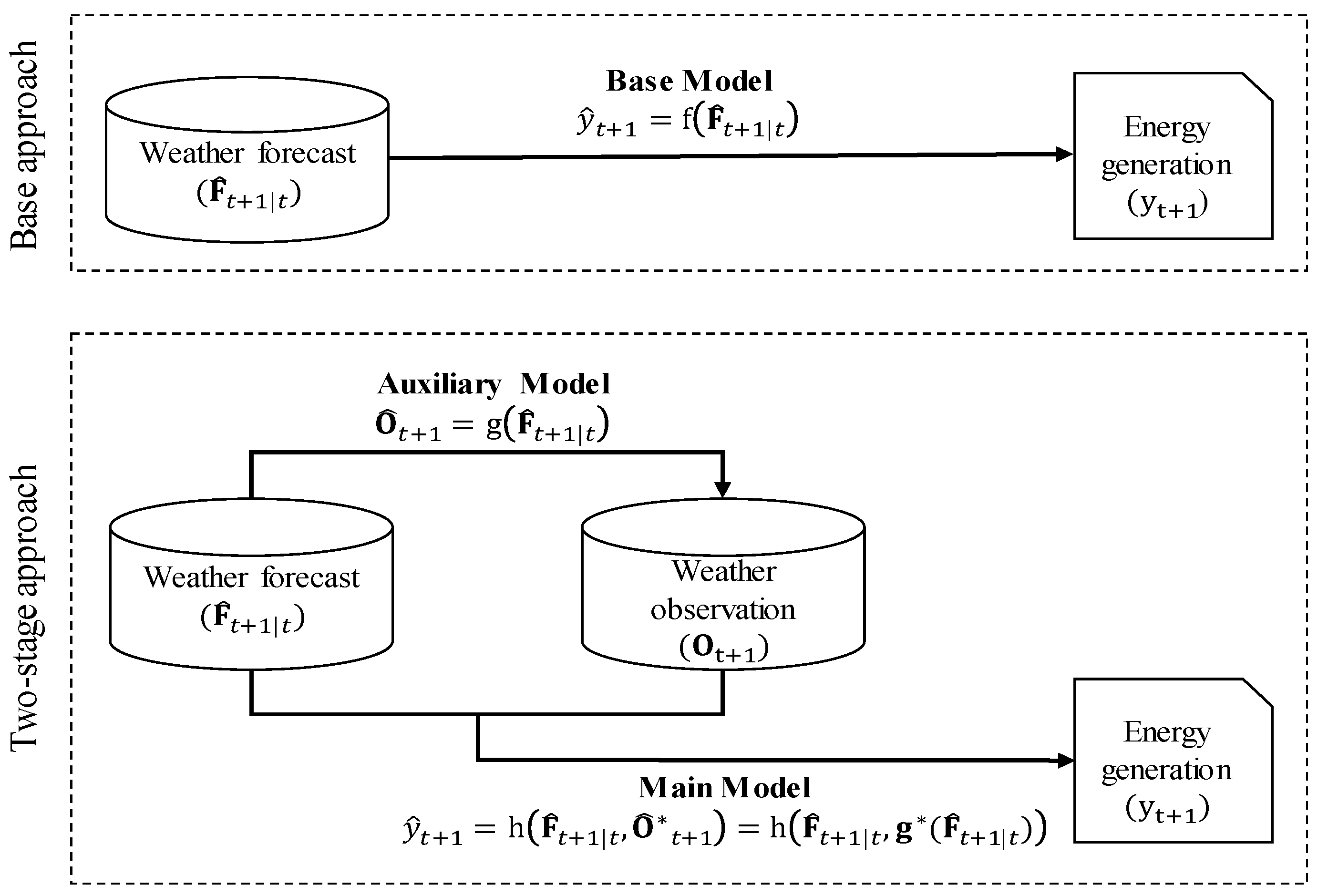
  • This study proposes an approach to expanding predictors for the prediction of solar power generation. It exemplifies a practical application to include relevant but delayed climatic data that are not available in real-time.
  • Many practical applications, including renewable energy operations, call for predictions using weather information as predictors. The proposed approach can be applied to predictions for renewable energy operations, such as wind, tide, and geothermal power production.
  • Generally, identifying latent variables and incorporating them in the prediction process often enhance the model performance. The proposed two-step approach does so with various machine learning algorithms.
  • In applications of machine learning methods, identifying latent variable structures in prior often enhances the performance of resulting models. This study indirectly investigates how much each machine learning algorithm gains benefit from the intermediate latent variable identification process.

2. Materials and Methods

This section describes the data set and methods used to develop the models. Section 2.1 describes the sources of the data and the preprocessing steps and Section 2.2 briefly explains the machine learning algorithms used in this study. Section 2.3 finally formulates the prediction problems that the three proposed models aim to solve.

2.1. Data Collection and Preprocessing

A solar power generation data from the Yeongam Photovoltaic Power Plant in South Korea were collected from a publicly available database (http://www.data.go.kr) provided by the government. The weather-related data were provided by the KMA. Solar elevation information was obtained from a database by the Stellarium®.
The variables in the dataset can be divided into four categories as listed in Table 1. First, hourly power generation data were collected. The hourly data excluded daylight-free hours (00:00–08:00 and 20:00–24:00) and were collected over three years from 2013-01-01 to 2015-12-31. Second, weather forecast data were collected. This study collected all available variables for the same period where power generation data were available during the corresponding period announced for the same period. The constructed models predicted future power generation amounts using weather forecast data announced for the future period. The KMA announced short-term weather forecasts at the city or district level for each three-hour period from 02:00 each day. We used the forecast data announced at 11:00 targeted for 09:00, 12:00, 15:00, and 18:00 of the following day (corresponding to 22, 25, 28, and 31 hours after the announcement, respectively). Solar elevation data were collected from an open source program called Stellarium (www.stellarium.org). Specifically, we estimated the solar elevation (0°–90°) for the same period using the latitude 34.751702 and longitude 126.458533, which is the geographical location of the power plant. The position of solar affects how much solar radiation energy is collected at the ground, along with other weather conditions, such as rain, snow, cloud, and the density of air. Third, actual weather records were obtained. This study included all-weather observation variables that were not included in weather forecasts. In the step of auxiliary modeling, this study built a prediction model for the weather observation variables (Radiation, VaporPressure, SurfaceTemperature, and AtmosphericPressure) using weather forecast data, called auxiliary variables in this research.
The preprocessing task prepared the data into the structure suitable for quantitative modeling. Categorical variables in the weather forecasts, such as RainfallType, SkyType, and WindDirection, were converted to multiple binary variables through one-hot coding. A week index variable (Weeknum) was created to reflect seasonal changes. This variable assigns index sequentially from the first week to the last week of each year. To include information about the time of the day, the variable TimeZone was used to indicate three-hour intervals.

2.2. Machine Learning Methods

This subsection briefly describes the machine learning methods tested in this study. The methods include popular supervised learning methods in the research line [4]. Linear regression is a simple but effective modeling technique where the linear relationship between independent variables and a dependent variable is to be identified. SVR is a variant of linear regression where prediction error that is smaller than some threshold is ignored in order to minimize the effect of outliers. Kernel functions, such as polynomial and radial basis functions, help the SVR perform the non-linear separation [26,34]. ANN is becoming an increasingly popular method for non-linear regression due to its effectiveness in data prediction. To find the relationship between input and output nodes, multi-layered hidden nodes are connected and their weights are updated through the error backpropagation algorithm [6,31,32,35,36]. CART, also known as recursive partitioning, splits an entire data set into two groups by searching for the best split condition that can reduce the sum of squared errors (SSE) mostly. This binary partitioning occurs recursively until each leaf node reaches to have enough impurity [27,37]. k-NN is a non-parametric method used for classification and regression [28,29]. For each instance, the predicted value is based on the weighted average value of the k neighborhood instances where each of the weight is commonly given as an inverse value of the distance between the target instance and each instance of the k nearest neighbors. Since k-NN treats input variables indiscriminately, this study scales and normalizes all the input instances in a preprocessing step.
As a representative ensemble learning method, AdaBoost fits additional copies of the decision tree but with the weights adjusted to the error of the current prediction. By subsequently focusing more on difficult instances, the learning mechanism boosts weaker learners to produce powerful “committees” [3]. Another powerful ensemble implementation is RFR, which consists of a collection of decision trees that are built from each bootstrapping sampling of the entire data set [30]. Averaging values from each tree, RFR generates a prediction value.
In the post-analysis, this study measures the Gini importance or the mean decrease in impurity (MDI) as an important measure to investigate the effect of each predictor. The Gini importance is defined as the total decrease in node impurity, averaged over all trees of the ensemble. By sorting the predictors using the Gini importance, the contribution of each predictor can be evaluated.

2.3. Problem Statements

In this study, we aimed to build a model that predicts solar power generation one day ahead of the actual operation. The base model identified the best function f * in which the predictors were limited to the weather forecast variables.
f * = a r g m i n f   L ( y t + 1 , y ^ t + 1 ) s . t .   y ^ t + 1 = f ( F ^ t + 1 | t )
where F ^ t + 1 | t is a vector of weather forecast variables available at day t and targeted for day t + 1 (The hat notation emphasizes that this quantity is forecasted.), y t + 1 is a quantity of power generation at day t + 1, and L is a cost function where this study adopted the measure of mean squared error (MSE) as a popular choice.
Though a few variables in weather observation were missing in weather forecasts, this study aimed to fully exploit weather information for building prediction process. That is, the weather observation variables were predicted using weather forecast variables. This auxiliary model aimed to find the best performing function g * , such as
g * = a r g m i n g   L ( O t + 1 , O ^ t + 1 ) s . t .   O ^ t + 1 = g ( F ^ t + 1 | t )
where O t + 1 is a vector of weather observation variables that are known to be related to solar power but not included in weather forecast [7,25].
Finally, the main model aimed to exploit the two previous models by including both O ^ t + 1 = g * ( F ^ t + 1 | t ) and F ^ t + 1 | t as predictors. The main model identified the best function h * such that
h * = a r g m i n h   L ( y t + 1 , y ^ t + 1 ) s . t .   y ^ t + 1 = h ( F ^ t + 1 | t ,   g * ( F ^ t + 1 | t ) )
where g * is obtained from the auxiliary model.
The base model provides a baseline for comparisons to the main model, which includes generated predictors. Since predictive relationships are complex and difficult to grasp, this study tests several machine learning algorithms, such as linear regression, SVR, CART, k-NN, AdaBoost, and RFR, which are suitable for the structure of the data and the problem. Before applying the machine learning algorithms, proper scaling is performed. Specifically, distance-based methods, including k-NN and SVR, need standardization so-called z-score normalization, in order to carry comparable importance in model generation process [34]. To calculate z-score, each variable x is subtracted by its mean μ and divided by its standard deviation σ, that is, z = (xμ)/σ. ANN needs a min-max scaling to a bounded range, such as between 0 and 1, in these experiments. The normalized value can be calculated by (xmin(x))/(max(x) − min(x)). This step is necessary so that all variables are in a comparable range before fed into a network [34]. Tree-based methods, such as AdaBoost, CART, and RFR, do not need scaling since they bisect each variable in a non-parametric manner [34]. Linear regression does not need to scale the data, either. By optimizing parameters under the train set, prediction models based on each machine learning algorithm are built with the machine learning package in Python, scikit-learn [38].

3. Results

This section presents the results of the methods described in the previous section. The results identify (1) which machine learning method produces the best-performing model, (2) whether the predicted values for auxiliary variables created during the auxiliary modeling step have significant forecasting performance for solar power generation, and (3) how much each independent variable among weather forecast and weather observation contributes to prediction performance. Section 3.1 explains the setting of experiments, Section 3.2 presents the performance of the auxiliary model formulated as Equation (2), and Section 3.3 compares performances of the base model in Equation (1) and the main model in Equation (3).

3.1. Measures for Model Comparison

To build models, the data for three years were split to a training set (30 months; from 2013-01-01 to 2015-06-30) and a test set (6 months; from 2015-07-01 to 2015-12-31). Using the train set, five-fold cross-validation was performed to find the best model for each prediction algorithm. The random search technique was adopted to search the proper parameter set of the best model.
An error measure of the mean squared error (MSE) was employed in choosing the best model among candidates. Specifically, the MSE measures an average value of squares of errors, formulated as:
M S E = 1 N i = 1 N ( y i y i ^ ) 2 = R M S E 2
where y i is the i-th actual value, y i ^ is the predicted value for y i , N is the number of samples, and RMSE implies the square root of MSE. Along with the MSE, this paper presents two other error measures, the R-squared value and the adjusted R-squared value. The R-squared value R 2 , also known as the coefficient of determination, is the proportion of the variance of the dependent variable that is explained by the independent variables.
R 2 = 1 i = 1 N ( y i y i ^ ) 2 i = 1 N ( y i y ¯ ) 2
where y ¯ is the mean of the actual values of y . The adjusted R-squared value, denoted R a d j 2 , penalizes the number of independent variables used to generate the predicted value, after measuring the proportion of the variance explained by independent variables.
R a d j 2 = 1 ( 1 R 2 ) N 1 N p 1
where p is the total number of the independent variables in the model.

3.2. Performance of Auxiliary Model

The proposed approach of this study features a two-step process, of which the first step predicts the observed variables ( O ) using the forecast variables ( F ^ ). The intermediate result created by this auxiliary model with RFR is presented in Table 2. Among four auxiliary variables, the prediction made on the first three variables, Radiation, VaporPressure, and SurfaceTemperature, are highly accurate with R2 higher than 97%. The other variable AtmosphericPressure also has generally acceptable accuracy. Having these auxiliary variables is equivalent to having another set of weather forecast when predicting the future solar power generation.

3.3. Performance of Base and Main Models

For the base model and the main model, popular machine learning algorithms in the line of studies are applied. Table 3, sorted by MSE in the main model, presents performances in the test set. It can be seen that R 2 for the test ranges from 57.9% to 70.1% in the base model, and from 67.2% to 70.5% in the main model. In the base model, RFR outperforms the others by large margins. Other methods exhibit similar performance except that k-NN performs poorly. In the main model, RFR still performs the best, but the margin is narrowed as other methods gain more from the two-step prediction process employed in the main model.
Figure 2 emphasizes the improvements in accuracy from utilizing the two-step process. By incorporating auxiliary variables ( O ) , each algorithm experiences an improvement as much as 9.7% ( R 2 of SVR). The best performing algorithm, RFR, gains 0.4% improvement in R 2 .
Figure 3 presents a time-series plot of predicted and actual values in a month (August 2015) of the test set. The predicted values are produced by the best RFR model with a parameter fitted by learning the train set. Overall, the predicted values track the fluctuations of actual power generation well, except for a series of under-predictions for the peak hour in early days in August and a big over-prediction on the peak hours on 22 August which is unavoidable by an unpredicted weather event. The day was unexpectedly foggy and heavily clouded (the maximally clouded day in August).
In the experiments on prediction models so far, all available variables in Table 1 are used. The advantages of the two-step approach are validated under this untouched setting. As a post analysis, the necessity of each predictor is assessed using a classical variable selection method, called backward elimination. Backward elimination starts with all variables, and a single variable is removed in each step until doing so would reduce the overall performance of the model. A performance measure R a d j 2 is used for this process, which penalizes the number of predictors so that a more concise model is promoted. Figure 4 presents which predictor is removed at each step.
The process begins with 25 predictors, including binary dummy variables, generated from categorical variables. This original model has a R a d j 2 value of 0.695. Excluding AtmosphericPressure would enhance the R a d j 2 value to 0.703, yielding a prediction model with 24 predictors. This weather variable for sea-level pressure turns out to be secondary to direct weather variables. Then, excluding WindDirection1 (West) and WindDirection2 (East) would enhance the R a d j 2 value to 0.711 and 0.713, respectively. Winds blowing from North or South carry more information compared to the winds blowing from East or West. No further removal is beneficial in terms of R a d j 2 . This process ensures some redundant, highly correlated or ineffective predictors to be removed. After the backward elimination process, the final model contains the smallest number of essential variables, but still achieves high prediction accuracy.

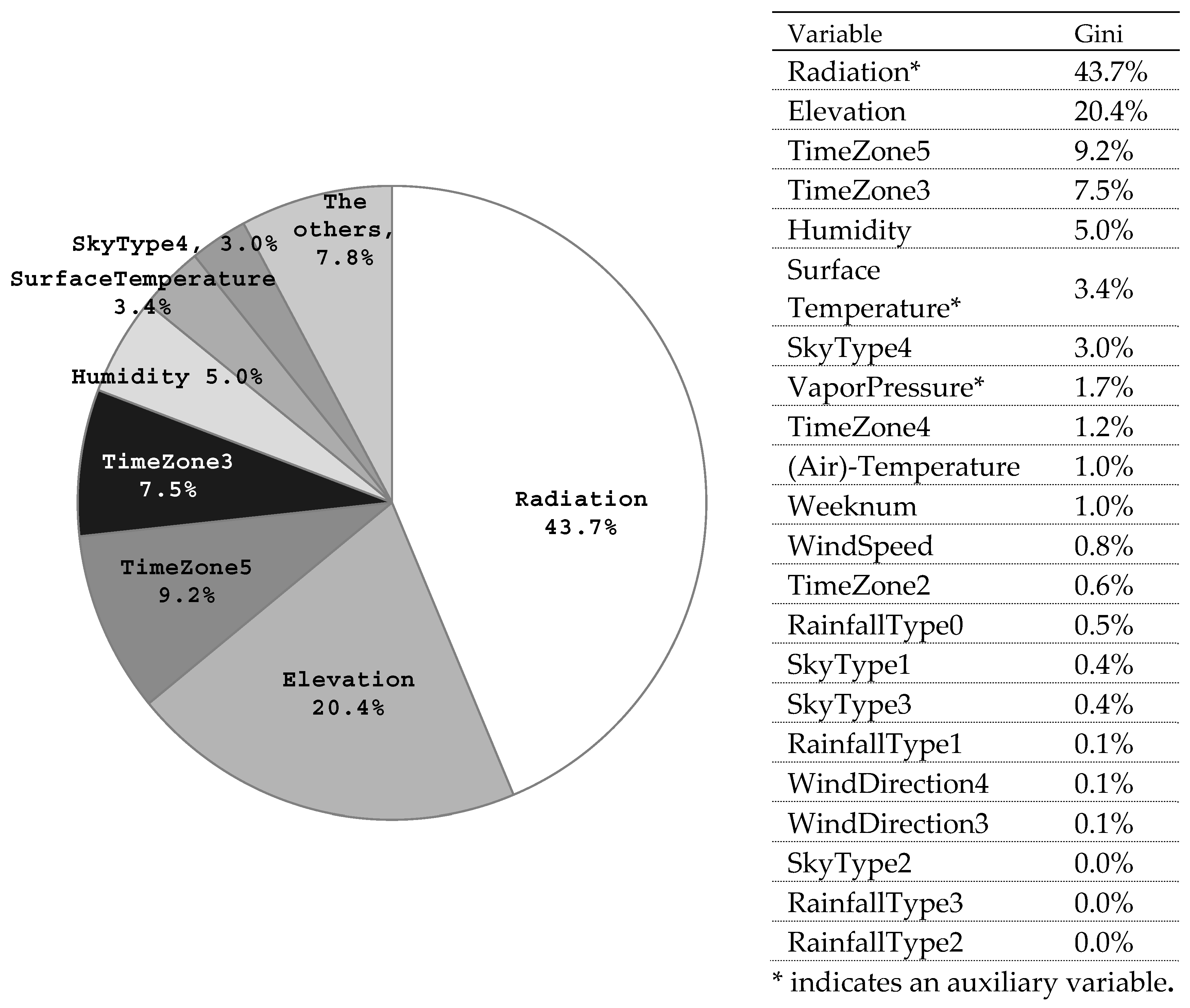
3.4. Importance of Variables

The above experiments demonstrate that the proposed two-step approach to solar power generation prediction improves the performance compared to the base model, regardless of the tested algorithms. Another way to validate its benefits is to measure whether the auxiliary variables are indeed pivotal components in the main model. Determining the necessary predictors, the importance of each variable in the final model is examined in the next subsection. Because the RFR model performs best, we adopt the Gini importance or mean decrease in impurity (MDI) as an important measure. The MDI is defined as the total decrease in node impurity, averaged over all trees of the ensemble. By sorting the predictors using the important measure, the contribution of each predictor is ranked.
Figure 5 presents the Gini importance of each variable in the main model with RFR. This figure supports the hypothesis for the benefit in the two-step process. One of the auxiliary variable, Radiation, is the most important variable with the importance of 43.7%. Other auxiliary variables, such as SurfaceTemperature and VaporPressure, are ranked in the upper half among all variables. The top four important variables consist of how much solar radiation is emitted (Radiation), from which solar position (Elevation), at what time of the day (TimeZone5 and TimeZone3). The condition of the air (Humidity) and temperatures (SurfaceTemperature and Air-Temperature) also affect solar power generation. Sky condition of overcast (SkyType4) also plays a role.

4. Discussion

For the prediction of solar power generation during operations, weather forecast variables are readily available. On the other hand, the auxiliary variables are not available to use. The auxiliary modeling step utilizes the historical data to identify the relationship between available forecasts and suitable predictions for the auxiliary variables. The generated predictions for the auxiliary variables using available forecasts are highly accurate (see Table 2). The main model utilizes the predicted values for the auxiliary variables along with available forecasts. On comparing the base models and the main models with popular machine learning algorithms, it is shown that the main models successfully improved the performance of the base models (see Table 3, Figure 2, and Figure 3). Among the tested machine learning algorithms, the models generated by RFR outperform the other models. The relative importance for each predictor is identified (see Figure 5) after the removal of a few variables (see Figure 4).
The results can be interpreted as follows:
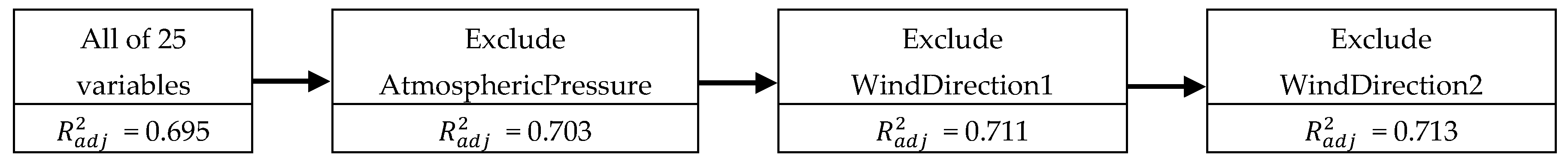
  • For predicting the solar power generation, the forecasts for the amount of solar radiation is the most important among the others, in terms of the Gini importance. The forecast for solar radiation is not directly available from the weather agency but can be indirectly generated by the proposed auxiliary model. Next, the position of the solar relative to the ground (Elevation) carries important information, and the operation time of the day affects the power generation. Since solar elevation can be accurately forecasted by astrophysics and the time of the day (TimeZone) is deterministic, the future information for these two variables are attainable accurately. The condition of the atmosphere (Humidity and VaporPressure) and the temperatures (SurfaceTemperature and Air-Temperature) also affect the power generation.
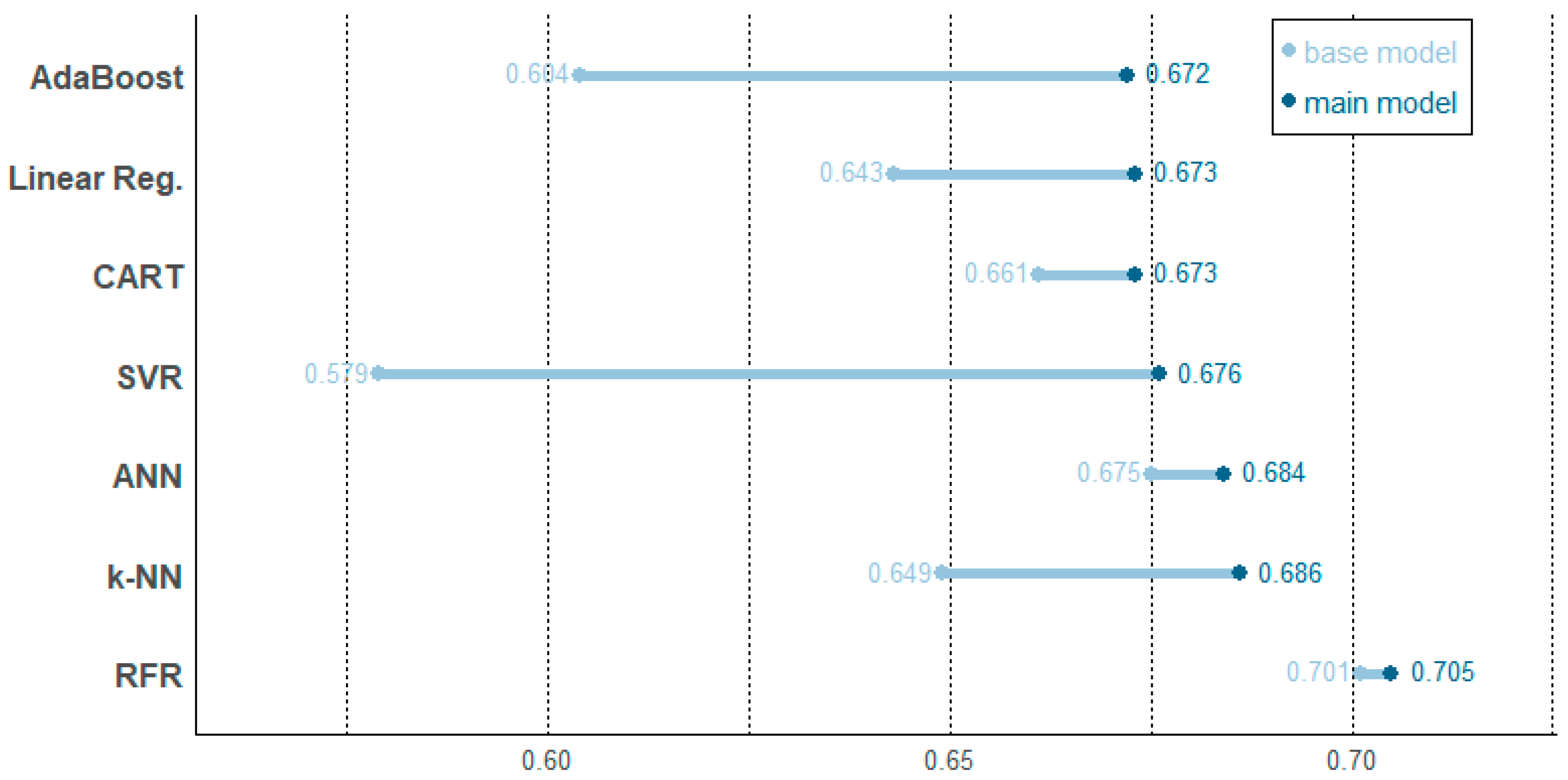
  • Forecasts for auxiliary variables are not readily available during actual power generation operations, but their values are later realized and highly correlated to the solar power generation. This relationship is captured by the auxiliary model, and the main model exploits this information to outperform the base model regardless of the machine learning methods applied. This approach, regarded as identification of latent variables, enhances the performances of solar power prediction.
  • On comparing the different machine learning methods, models with higher capacity, such as RFR, k-NN, and ANN, perform relatively well. RFR, the best performing method, is characterized by its ensemble approach with multiple randomized trees and known for its robustness in the test data set. It is generally known that RFR is especially suitable when multiple categorical variables are involved, as in our case. The main results support the robustness and good performance of RFR.

5. Conclusions

This study proposes a two-step approach to solar power generation prediction to fully exploit the information contained in the weather data. Specifically, the predicted values for auxiliary variables contribute greatly to enhancing prediction performance.
Studies in this line present a wide range of errors from 3% to 38% [4]. The large over-prediction on 22 August due to an unexpected weather event (see Figure 3) indicates how the error distribution can be highly skewed. Skewed errors result in lower overall accuracy, especially for the power plant located in areas of unpredictable weather. In particular, the power plant of this study is located in a landfill area in the southwestern part of the Korean peninsula, which is surrounded by three seas and 70% of whose total area is mountainous, making weather predictions very difficult. To aid actual operations, it would be meaningful in future studies, especially for areas with low weather predictability, to present confidence intervals of the predicted value, as well as the predicted values themselves.
This paper exemplifies a practical application of feature extraction such that latent variables, relevant but delayed weather data in this study, are identified prior to the main modeling. This study validates that the process of latent structure identification improves the solar power generation problem and aids PV plant operations.
Furthermore, other renewable energy operations, such as wind, tide, and geothermal power production, can also be benefitted from the proposed approach. More generally, it can also be applied to other fields that require predicting future weather conditions.

Author Contributions

S.-G.K. and J.-Y.J. designed the research purposes and methodology; S.-G.K. developed the software that is validated and further developed by M.K.S.; S.-G.K. and M.K.S. analyzed the data; S.-G.K. and M.K.S. wrote the original draft; M.K.S. and J.-Y.J. reviewed and finalized the draft. This research project was conducted under the supervision of J.-Y.J.

Funding

This work was supported by the National Research Foundation of Korea (NRF) grant funded by the Korea government (MSIT) (NRF-2017H1D8A2031138).

Conflicts of Interest

The authors declare no conflict of interest.

Appendix A. Candidates and Optimal Values of Proposed Models

This appendix section presents tables for illustrating hyperparameter tuning process for each model proposed in this study.
Table A1. Hyperparameter candidates and optimal values for the base model.
MethodSet of Considered Hyperparameters (The Selected Value is in the Gray Box)Description
AdaBoost Sustainability 11 01501 i001The maximum number of estimators at which boosting is terminated.
Learning rate of shrinking the contribution of each regressor.
The loss function to use when updating the weights after each boosting iteration.
Linear Reg.fit_intercept = TrueWhether to calculate the intercept for this model.
CART Sustainability 11 01501 i002The maximum depth of the tree.
The number of features to consider when looking for the best split.
The minimum number of samples required to split an internal node.
The minimum number of samples required to be at a leaf node.
SVR Sustainability 11 01501 i003Penalty parameter C of the error term.
ANN Sustainability 11 01501 i004The number of neurons in a single hidden layer.
The activation function for the hidden layer.
Learning rate schedule for weight updates.
The maximum number of iterations.
k-NN Sustainability 11 01501 i005The number of neighbors to use by default.
The algorithm used to compute the nearest neighbors.
Weight function used in the prediction
RFR Sustainability 11 01501 i006The number of trees in the forest.
The maximum depth of the tree.
The number of features to consider when looking for the best split.
The minimum number of samples required to split an internal node.
The minimum number of samples required to be at a leaf node.
Table A2. Hyperparameter candidates and optimal values for the auxiliary models with the random forest regression method.
RadiationVapor Pressure
Sustainability 11 01501 i007 Sustainability 11 01501 i008
Surface TemperatureAtmospheric Pressure
Sustainability 11 01501 i009 Sustainability 11 01501 i010
Table A3. Hyperparameter candidates and optimal values for the main model.
MethodSet of Considered Hyperparameters (The Selected Value is in the Gray Box)Description
AdaBoost Sustainability 11 01501 i011The maximum number of estimators at which boosting is terminated.
Learning rate of shrinking the contribution of each regressor.
The loss function to use when updating the weights after each boosting iteration.
Linear Reg.fit_intercept = TrueWhether to calculate the intercept for this model.
CART Sustainability 11 01501 i012The maximum depth of the tree.
The number of features to consider when looking for the best split.
The minimum number of samples required to split an internal node.
The minimum number of samples required to be at a leaf node.
SVR Sustainability 11 01501 i013Penalty parameter C of the error term.
ANN Sustainability 11 01501 i014The number of neurons in a single hidden layer.
The activation function for the hidden layer.
Learning rate schedule for weight updates.
The maximum number of iterations.
k-NN Sustainability 11 01501 i015The number of neighbors to use by default.
The algorithm used to compute the nearest neighbors.
Weight function used in the prediction.
RFR Sustainability 11 01501 i016The number of trees in the forest.
The maximum depth of the tree.
The number of features to consider when looking for the best split.
The minimum number of samples required to split an internal node.
The minimum number of samples required to be at a leaf node.

References

  1. Kim, S.; Jung, J.-Y.; Sim, M. Machine Learning Methods for Solar Power Generation Prediction based on Weather Forecast. In Proceedings of the 6th International Conference on Big Data Applications and Services (BigDAS2018), Zhengzhou, China, 19–22 August 2018. [Google Scholar]
  2. Suri, M.; Huld, T.; Dunlop, E.D. Geographic aspects of photovoltaics in Europe: Contribution of the PVGIS website. IEEE J. Sel. Top. Appl. Earth Obs. Remote Sens. 2008, 1, 34–41. [Google Scholar] [CrossRef]
  3. Antonanzas, J.; Osorio, N.; Escobar, R.; Urraca, R.; Martinez-de-Pison, F.J.; Antonanzas-Torres, F. Review of photovoltaic power forecasting. Sol. Energy 2016, 15, 78–111. [Google Scholar] [CrossRef]
  4. Voyant, C.; Notton, G.; Kalogirou, S.; Nivet, M.L.; Paoli, C.; Motte, F.; Fouilloy, A. Machine learning methods for solar radiation forecasting: A review. Renew. Energy 2017, 1, 569–582. [Google Scholar] [CrossRef]
  5. Abedinia, O.; Raisz, D.; Amjady, N. Effective prediction model for Hungarian small-scale solar power output. IET Renew. Power Gener. 2017, 11, 1648–1658. [Google Scholar] [CrossRef]
  6. Abuella, M.; Chowdhury, B. Improving Combined Solar Power Forecasts Using Estimated Ramp Rates: Data-driven Post-processing Approach. IET Renew. Power Gener. 2018, 12, 1127–1135. [Google Scholar] [CrossRef]
  7. Chaouachi, A.; Kamel, R.M.; Nagasaka, K. Neural network ensemble-based solar power generation short-term forecasting. J. Adv. Comput. Intell. Intell. Inform. 2010, 14, 69–75. [Google Scholar] [CrossRef]
  8. Hossain, M.R.; Oo, A.M.; Ali, A.S. Hybrid prediction method of solar power using different computational intelligence algorithms. In Proceedings of the Power Engineering Conference (AUPEC), Christchurch, New Zealand, 26 September 2012. [Google Scholar]
  9. Li, L.L.; Cheng, P.; Lin, H.C.; Dong, H. Short-term output power forecasting of photovoltaic systems based on the deep belief net. Adv. Mech. Eng. 2017, 9, 1687814017715983. [Google Scholar] [CrossRef]
  10. David, M.; Ramahatana, F.; Trombe, P.J.; Lauret, P. Probabilistic forecasting of the solar irradiance with recursive ARMA and GARCH models. Sol. Energy 2016, 133, 55–72. [Google Scholar] [CrossRef] [Green Version]
  11. Pedro, H.T.; Coimbra, C.F. Assessment of forecasting techniques for solar power production with no exogenous inputs. Sol. Energy 2012, 86, 2017–2028. [Google Scholar] [CrossRef]
  12. Phinikarides, A.; Makrides, G.; Kindyni, N.; Kyprianou, A.; Georghiou, G.E. ARIMA modeling of the performance of different photovoltaic technologies. In Proceedings of the 39th Photovoltaic Specialists Conference (PVSC), Tampa, FL, USA, 16–21 June 2013. [Google Scholar]
  13. Hassan, J. ARIMA and regression models for prediction of daily and monthly clearness index. Renew. Energy 2014, 68, 421–427. [Google Scholar] [CrossRef]
  14. Alzahrani, A.; Shamsi, P.; Dagli, C.; Ferdowsi, M. Solar irradiance forecasting using deep neural networks. Procedia Comput. Sci. 2017, 114, 304–313. [Google Scholar] [CrossRef]
  15. Abdel-Nasser, M.; Mahmoud, K. Accurate photovoltaic power forecasting models using deep LSTM-RNN. Neural Comput. Appl. 2017, 1–4. [Google Scholar] [CrossRef]
  16. Sharma, N.; Gummeson, J.; Irwin, D.; Shenoy, P. Cloudy computing: Leveraging weather forecasts in energy harvesting sensor systems. In Proceedings of the 7th Annual IEEE Communications Society Conference, Sensor Mesh and Ad Hoc Communications and Networks (SECON), Boston, MA, USA, 21 June 2010. [Google Scholar]
  17. Sharma, N.; Sharma, P.; Irwin, D.; Shenoy, P. Predicting solar generation from weather forecasts using machine learning. In Proceedings of the 2nd IEEE International Conference, Smart Grid Communications (SmartGridComm), Brussels, Belgium, 17–20 October 2011. [Google Scholar]
  18. Amrouche, B.; Le Pivert, X. Artificial neural network based daily local forecasting for global solar radiation. Appl. Energy 2014, 130, 333–341. [Google Scholar] [CrossRef]
  19. Zamo, M.; Mestre, O.; Arbogast, P.; Pannekoucke, O. A benchmark of statistical regression methods for short-term forecasting of photovoltaic electricity production, part I: Deterministic forecast of hourly production. Sol. Energy 2014, 105, 792–803. [Google Scholar] [CrossRef]
  20. Gensler, A.; Henze, J.; Sick, B.; Raabe, N. Deep Learning for solar power forecasting-An approach using AutoEncoder and LSTM Neural Networks. In Proceedings of the 2016 IEEE International Conference, Systems, Man, and Cybernetics (SMC), Budapest, Hungary, 9 October 2016. [Google Scholar]
  21. Andrade, J.R.; Bessa, R.J. Improving renewable energy forecasting with a grid of numerical weather predictions. IEEE Trans. Sustain. Energy 2017, 8, 1571–1580. [Google Scholar] [CrossRef]
  22. Leva, S.; Dolara, A.; Grimaccia, F.; Mussetta, M.; Ogliari, E. Analysis and validation of 24 hours ahead neural network forecasting of photovoltaic output power. Math. Comput. Simul. 2017, 131, 88–100. [Google Scholar] [CrossRef] [Green Version]
  23. Persson, C.; Bacher, P.; Shiga, T.; Madsen, H. Multi-site solar power forecasting using gradient boosted regression trees. Sol. Energy 2017, 150, 423–436. [Google Scholar] [CrossRef]
  24. Detyniecki, M.; Marsala, C.; Krishnan, A.; Siegel, M. Weather-based solar energy prediction. In Proceedings of the 2012 IEEE International Conference, Fuzzy Systems (FUZZ-IEEE), Brisbane, Australia, 10 June 2012. [Google Scholar]
  25. Bacher, P.; Madsen, H.; Nielsen, H.A. Online short-term solar power forecasting. Sol. Energy 2009, 83, 1772–1783. [Google Scholar] [CrossRef] [Green Version]
  26. Sharma, S.; Jain, K.K.; Sharma, A. Solar cells: In research and applications—A review. Mater. Sci. Appl. 2015, 6, 1145. [Google Scholar] [CrossRef]
  27. Mori, H.; Takahashi, A. A data mining method for selecting input variables for forecasting model of global solar radiation. In Proceedings of the 2012 IEEE PES, Transmission and Distribution Conference and Exposition (T&D), Orlando, FL, USA, 7–10 May 2012. [Google Scholar]
  28. Voyant, C.; Paoli, C.; Muselli, M.; Nivet, M.L. Multi-horizon solar radiation forecasting for Mediterranean locations using time series models. Renew. Sustain. Energy Rev. 2013, 28, 44–52. [Google Scholar] [CrossRef]
  29. Pedro, H.T.; Coimbra, C.F. Nearest-neighbor methodology for prediction of intra-hour global horizontal and direct normal irradiances. Renew. Energy 2015, 80, 770–782. [Google Scholar] [CrossRef]
  30. Lee, K.; Kim, W.J. Forecasting of 24 hours Ahead Photovoltaic Power Output Using Support Vector Regression. J. Korean Inst. Inf. Technol. 2016, 14, 175–183. [Google Scholar] [CrossRef]
  31. Almeida, M.P.; Perpinan, O.; Narvarte, L. PV power forecast using a nonparametric PV model. Sol. Energy 2015, 115, 354–368. [Google Scholar] [CrossRef] [Green Version]
  32. Song, J.J.; Jeong, Y.S.; Lee, S.H. Analysis of prediction model for solar power generation. J. Digit. Converg. 2014, 12, 243–248. [Google Scholar] [CrossRef] [Green Version]
  33. Yona, A.; Senjyu, T.; Funabshi, T.; Sekine, H. Application of neural network to 24-hours-ahead generating power forecasting for PV system. IEEJ Trans. Power Energy 2008, 128, 33–39. [Google Scholar] [CrossRef]
  34. Kuhn, M.; Johnson, K. Appl. Predict. Model, 1st ed.; Springer: New York, NY, USA, 2013. [Google Scholar]
  35. Voyant, C.; Soubdhan, T.; Lauret, P.; David, M.; Muselli, M. Statistical parameters as a means to a priori assess the accuracy of solar forecasting models. Energy 2015, 90, 671–679. [Google Scholar] [CrossRef] [Green Version]
  36. Kalogirou, S.A. Artificial neural networks in renewable energy systems applications: A review. Renew. Sustain. Energy Rev. 2001, 5, 373–401. [Google Scholar] [CrossRef]
  37. Breiman, L. Classification and Regression Trees, 1st ed.; Routledge: New York, NY, USA, 1984. [Google Scholar]
  38. Pedregosa, F.; Varoquaux, G.; Gramfort, A.; Michel, V.; Thirion, B.; Grisel, O.; Blondel, M.; Prettenhofer, P.; Weiss, R.; Dubourg, V.; Vanderplas, J. Scikit-learn: Machine learning in Python. J. Mach. Learn. Res. 2011, 12, 2825–2830. [Google Scholar]
Figure 1. The base model and the proposed two-step approach for solar power generation prediction based on weather data.
Sustainability 11 01501 g001
Figure 2. Improved prediction performance in terms of R2 from the base model to the main model.
Sustainability 11 01501 g002
Figure 3. Actual values and predicted values by RFR from 1 August to 31 August 2015.
Sustainability 11 01501 g003
Figure 4. Backward elimination process with the RFR model.
Sustainability 11 01501 g004
Figure 5. Gini importance of variables in the main model based on RFR.
Sustainability 11 01501 g005
Table 1. Dependent and Independent Variables 1.
SourceVariable NameDescription
Dependent variablePower plant ( y ) GenerationSolar power generation (kWh)
Independent variableWeather forecast ( F ^ ) RainfallType0: none, 1: rain, 2: rain/snow, 3: snow
SkyType1: sunny, 2: a little cloudy, 3: cloudy, 4: overcast
WindDirection1: west, 2: east, 3: south, 4: north
WindSpeedWind speed (m/s)
HumidityHumidity (%)
TemperatureTemperature (°C)
ElevationSolar Elevation (0°–90°) by Stellarium®
Weather observation ( O ) RadiationRadiation (MJ/m2)
VaporPressureVapor pressure (hPa)
SurfaceTemperatureSurface temperature (°C)
AtmosphericPressureAtmospheric Pressure (hPa)
Derived variablesWeeknumWeekly index (1–53)
TimeZone1: 09:00–12:00, 2: 12:00–15:00,
3: 15:00–18:00, 4: 18:00–21:00
1 The total number of available observations is 4380 (1095 days × 4 observations/day).
Table 2. Performance of the auxiliary model on the test set.
R M S E R 2
Radiation0.12897.0
VaporPressure0.74399.3
SurfaceTemperature1.25298.7
AtmosphericPressure4.28872.4
1 See Table A2 for selected hyperparameters to generate the models.
Table 3. Performance of the base model and the main model in the test set.
AlgorithmBase ModelMain ModelImprovement
RMSE R 2 RMSE R 2 RMSE R 2
AdaBoost669.50.604609.20.67260.3 (9.0%)0.068
Linear Reg.635.50.643608.60.67326.9 (4.2%)0.030
CART619.20.661607.90.67311.3 (−1.8%)0.012
SVR689.90.579605.70.67684.2 (12.2%)0.097
ANN606.00.675597.40.684−8.6 (1.4%)0.009
k-NN630.20.649596.40.686−35.8 (5.7%)0.037
RFR581.50.701577.50.7054.0 (−0.7%)0.004
2 Algorithms are ordered by R 2 of the main model, 3 See Table A1 and Table A3 for selected hyperparameters to generate the models.

