Cost Adjustment in the Korean Defense Industry: Empirical Research on the Relation between Earnings Management and Sustainability


Abstract
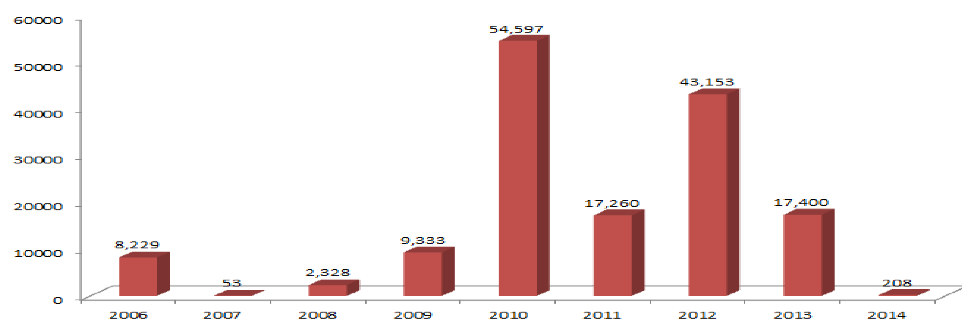
1. Introduction
2. Prior Research and Different Concepts of Earnings Management
3. Hypotheses and Research Design
3.1. Hypotheses
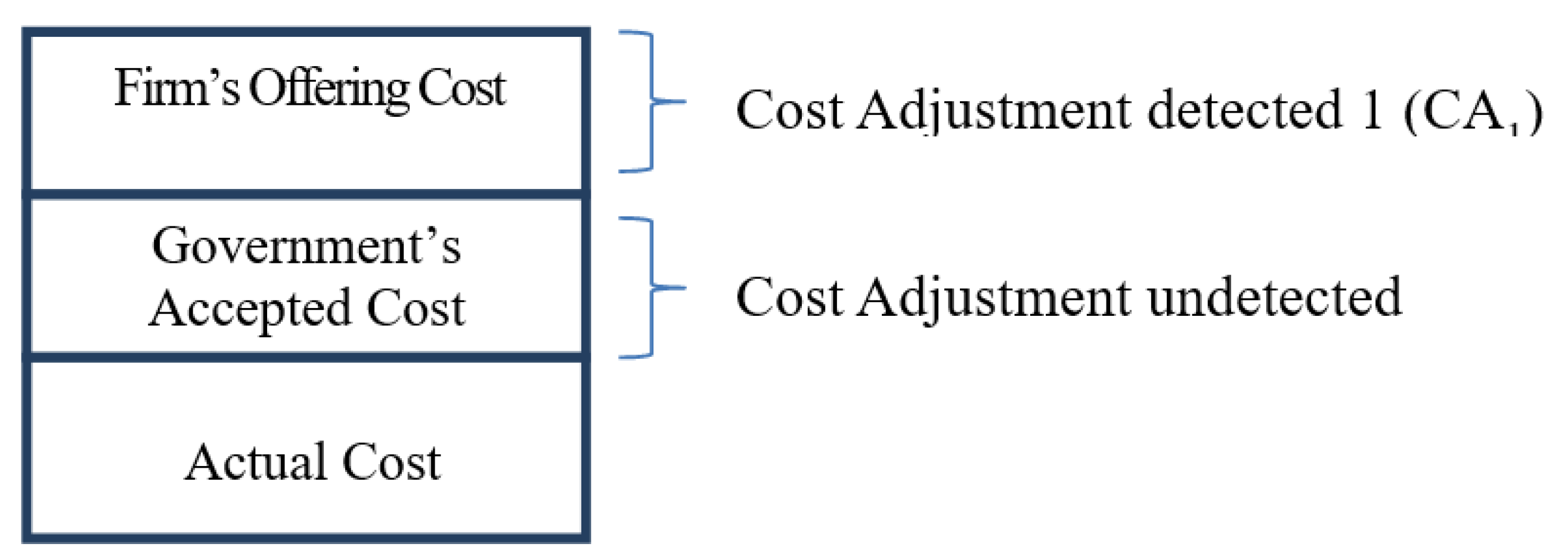
3.2. Cost Adjustment Detection
3.3. Conventional Relationship between ‘CA (Cost Adjustment)’ Variable and Prior Earnings Management Incentives
3.4. Main Research Model and Variable Definitions
β6LEVi,t + β7GROWTHi,t + β8MTBi,t−1 + Yeari,tdummy + Indi,tdummy+ εi,t.
β5LEVi,t + β6GROWTHi,t + β7MTBi,t−1 + Yeari,tdummy + Indi,tdummy + εi,t.
4. Sample Selection and Results
4.1. Sample Selection
4.2. Data Deduction
| - E(Rj) | Cost of equity capital for firmj |
| - Rf | Risk free rate |
| - E(Rm) | Market risk premium |
| - βj | Market risk coefficient, systematic risk for firmj |
4.3. Descriptive Statistics
4.4. Empirical Results
5. Robust Test
Ridge Regression
6. Conclusions
Author Contributions
Funding
Acknowledgments
Conflicts of Interest
References
- SIPRI. Available online: https://www.books.sipris.org/files/FS/SPIRIFS1604.pdf (accessed on 12 August 2016).
- Defense Acquisition Program Administration Internal Report; DAPA: Gwacheon-si, Korea, 2014.
- Defense Acquisition Program Administration Internal Report; DAPA: Gwacheon-si, Korea, 2008.
- Rogerson, W.P. Overhead Allocation and Incentives for Cost Minimization in Defense Procurement. Account. Rev. 1992, 67, 671–691. [Google Scholar]
- KDIA. Available online: http://www.kdia.or.kr/content/3/2/4/view.do (accessed on 13 December 2015).
- Defense News. Available online: https://www.defensenews.com/industry/2018/10/04/t-x-loss-casts-shadow-over-south-korean-arms-exports/ (accessed on 19 February 2019).
- Hepworth, S.R. Smoothing periodic income. Account. Rev. 1953, 28, 32–39. [Google Scholar]
- Gordon, M.J. Postulates, principles and research in accounting. Account. Rev. 1964, 39, 251. [Google Scholar]
- Beidleman, C.R. Income smoothing: The role of management. Account. Rev. 1973, 48, 653–667. [Google Scholar]
- Moses, O.D. Income smoothing and incentives: Empirical tests using accounting changes. Account. Rev. 1987, 62, 358–377. [Google Scholar]
- Tucker, J.W.; Zarowin, P.A. Does income smoothing improve earnings informativeness? Account. Rev. 2006, 81, 251–270. [Google Scholar] [CrossRef]
- Bowen, R.M.; DuCharme, L.; Shores, D. Stakeholders’ implicit claims and accounting method choice. J. Account. Econ. 1995, 20, 255–295. [Google Scholar] [CrossRef]
- De Jong, A.; Mertens, G.; van der Poel, M.; van Dijk, R. How does earnings management influence investor’s perceptions of firm value? Survey evidence from financial analysts. Rev. Account. Stud. 2014, 19, 606–627. [Google Scholar] [CrossRef]
- Healy, P.M. The effect of bonus schemes on accounting decisions. J. Account. Econ. 1985, 7, 85–107. [Google Scholar] [CrossRef]
- Roychowdhury, S. Earnings management through real activities manipulation. J. Account. Econ. 2006, 42, 335–370. [Google Scholar] [CrossRef]
- Leuz, C.; Nanda, D.; Wysocki, P.D. Earnings management and investor protection: An international comparison. J. Financ. Econ. 2003, 69, 505–527. [Google Scholar] [CrossRef]
- Cheng, Q.; Warfield, T.D. Equity incentives and earnings management. Account. Rev. 2005, 80, 441–476. [Google Scholar] [CrossRef]
- Bergstresser, D.; Philippon, T. CEO incentives and earnings management. J. Financ. Econ. 2006, 80, 511–529. [Google Scholar] [CrossRef]
- Jones, J. Earnings management during import relief investigation. J. Account. Res. 1991, 29, 193–228. [Google Scholar] [CrossRef]
- Phillips, J.; Pincus, M.; Rego, S.O. Earnings management: New evidence based on deferred tax expense. Account. Rev. 2003, 78, 491–521. [Google Scholar] [CrossRef]
- Dhaliwal, D.S.; Gleason, C.A.; Mills, L.F. Last-chance earnings management: Using the tax expense to meet analysts’ forecasts. Contemp. Account. Res. 2004, 21, 431–459. [Google Scholar] [CrossRef]
- Badertscher, B.A.; Phillips, J.D.; Pincus, M.; Rego, S.O. Earnings management strategies and the trade-off between tax benefits and detection risk: To conform or not to conform? Account. Rev. 2009, 84, 63–97. [Google Scholar] [CrossRef]
- Kim, J.-B.; Sohn, B. Real earnings management and cost of capital. J. Account. Public Policy 2013, 32, 518–543. [Google Scholar] [CrossRef]
- Lee, J.-S. The Information Asymmetry and the Cost Stickiness Behavior in the Defense Industry. Ph.D. Thesis, The Graduate School of Kwangwoon University, Seoul, Korea, 2014. [Google Scholar]
- Kim, D.-U.; Jung, H.-R. A Study on Cost Structure of Korean Defense Firms. Q. J. Def. Policy Stud. 2012, 97, 109–143. [Google Scholar]
- Yoon, S.-M. Does Korean Defense Industry Manage Earnings? Master’s Thesis, Graduate School of SNU, Seoul, Korea, 2006. [Google Scholar]
- Ahn, T.-S.; Heo, E.-J. Costing and Pricing Rules and Their Impact on the Incentives of Defense Contractors. Korean Account. J. 2003, 12, 35–60. [Google Scholar]
- Tomas, J.K.; Tung, S. Cost Manipulation Incentives under Cost Reimbursement: Pension Cost for Defense Contracts. Account. Rev. 1992, 67, 691–711. [Google Scholar]
- Shin, H.-Y.; Koh, K.-S.; Lee, M.-Y. A Study on the Improvement of Defense Contracts and Cost Accounting Systems. J. Account. Financ. 2007, 25, 133–160. [Google Scholar]
- Forbes. Available online: http://www.forbes.com/forbes/1997/0210/5903097a.html (accessed on 26 August 2016).
- Defense Acquisition Program Administration Internal Report; DAPA: Gwacheon-si, Korea, 2012.
- Park, J.-Y.; Kim, S.-H.; Kim, D.-H. The effect of defense industry contract types on earnings management. Korean J. Account. Res. 2014, 19, 75–97. [Google Scholar]
- Plumlee, M.A. Discussion of the Effect of Information on Uncertainty and the Cost of Capital. Contemp. Account. Res. 2016, 33, 775–782. [Google Scholar] [CrossRef]
- Subrahmanyam, A.; Titman, A. Feedback from Stock Prices to Cash Flows. J. Financ. 2002, 56, 2389–2414. [Google Scholar] [CrossRef]
- Koo, J.H. The Effect of Earnings Management and Corporate Governance on the Cost Behavior. Ph.D. Thesis, The Graduate School of Sung Kyun Wan University, Seoul, Korea, 2009. [Google Scholar]
- Watts, R.L.; Zimmerman, J.L. Positive Accounting Theory; Prentice-Hall: Englewood Cliffs, NJ, USA, 1986. [Google Scholar]
- DeFond, M.L.; Jiambalvo, J. Debt Covenant Violation and Manipulation of Accruals. J. Account. Econ. 1996, 17, 145–176. [Google Scholar] [CrossRef]
- Dechow, P.M.; Sloan, R.; Sweeney, A. Detecting earnings management. Account. Rev. 1995, 70, 193–225. [Google Scholar]
- Watts, R.L.; Zimmerman, J.L. Toward a Positive Theory of the Determination of Accounting Standards. Account. Rev. 1978, 53, 112–134. [Google Scholar]
- DeAngelo, H.; DeAngelo, L.; Skinner, D.J. Accounting choice in troubled Companies. J. Account. Econ. 1994, 17, 113–144. [Google Scholar] [CrossRef]
- Skinner, D.J.; Sloan, R.G. Earnings surprises, growth expectations and stock returns or don’t let an earnings torpedo sink your portfolio. Rev. Account. Stud. 2002, 7, 289–312. [Google Scholar] [CrossRef]
- Dechow, P.M.; Sloan, R.; Sweeney, A. Causes and consequences of earnings manipulation: An analysis of firms subject to enforcement actions by the SEC. Contemp. Account. Res. 1996, 13, 1–36. [Google Scholar] [CrossRef]
- Edwards, A.; Schwab, C.; Shevlin, T. Financial Constraints and Cash Tax Savings. Account. Rev. 2016, 91, 859–881. [Google Scholar] [CrossRef]
- Park, J.-H.; Sohn, S.-K.; Jin, S.-H. A Study on the Optimum level operating Margin for Korean Defense Industry. Bus. Educ. Res. 2015, 29, 455–475. [Google Scholar]
- Modigliani, F.; Miller, M.H. The Cost of Capital, Corporation Finance and the Theory of Investment. Am. Econ. Rev. 1958, 48, 261–297. [Google Scholar]
- Ko, C.-Y.; Jung, H.; Park, J.-H. Estimating the Divisional Cost of Capital—Focusing on the Telecommunications. Korean Account. J. 2014, 23, 523–549. [Google Scholar]
- ECOS. Available online: http://ecos.bok.or.kr/ (accessed on 12 August 2016).
- Brambor, T.; Clark, W.; Gloder, M. Understanding interaction models: Improving empirical analyses. Political Anal. 2006, 14, 63–82. [Google Scholar] [CrossRef]


| When cost adjustment is undetected | Cost inflation → Weakening price or export competitiveness → Long-term Sustainability is impaired |
| When Illegal cost adjustment is detected | Penalties imposed → Deteriorating reputation → Worsening business environment → Long-term or short-term sustainability is impaired |
| Prior study | Incentive for earnings management → Earnings management through cost decrease to increase income → ‘Quality of income’ decrease → ‘Accounting quality’ decrease → Reliability decrease → Cost of capital increase [23] |
| This study | Incentive for earnings management (Shareholder’s demand in income raise etc.) → Cost of capital increase → Adjustment of target income → Earnings management through expense increase to increase income → Cost increase → Maximization of compensation under cost-plus system → Maximization of the market value of equity |
| Variables | Specification | |
|---|---|---|
| Models 1–3 | CA1i,t | Total cost gap between firm offered and government accepted (|Total Costtfirm − Total Costtgov’t|)/Assett−1 |
| CECi,t−1 | Explanatory variable, lagged cost of equity capital | |
| PROFi,t | Dummy variable, if firms run by professional manager 1, or 0 | |
| ROAi,t | ‘NIt/Assett−1′ adjusted by the defense department | |
| SIZEi,t | Log value of the initial assets adjusted by the defense department Ln(Assett−1) | |
| LEVi,t | ‘Debtt/Assett−1′ adjusted by the defense department | |
| GROWTHi,t | Growth of sales adjusted by the defense department ΔSalest/Assett−1 | |
| MTBi,t−1 | The initial market value to the initial book value ratio Market valuet/Book valuet−1 | |
| Yeardummy | Year dummy variable | |
| Inddummy | Industry dummy variable | |
| Models 4–5 | CA2i,t | Total cost ratio of firm compared to government Ln(Total Costt firm/Total Costt gov’t) |
| Directi,t | All direct cost group ratio of firm side compared to government side Ln(All the Direct Costt firm/All the Direct Costtgov’t) | |
| Indirecti,t | All indirect cost group ratio of firm side compared to government side Ln(All the Indirect Costtfirm/All the Indirect Costtgov’t) | |
| DMCi,t | Direct material cost ratio of firm compared to government Ln(Direct Material Costtfirm/Direct Material Costtgov’t) | |
| IMCi,t | Indirect material cost ratio of firm compared to government Ln(Indirect Material Costtfirm/Indirect Material Costtgov’t) | |
| DLCi,t | Direct labor cost ratio of firm compared to government Ln(Direct Labor Costtfirm/Direct Labor Costtgov’t) | |
| ILCi,t | Indirect labor cost ratio of firm compared to government Ln(Indirect Labor Costtfirm/Indirect Labor Costtgov’t) | |
| DOCi,t | Direct other cost ratio of firm compared to government Ln(Direct Overhead Costtfirm/Direct Overhead Costtgov’t) | |
| IOCi,t | Indirect other cost ratio of firm compared to government Ln(Indirect Overhead Costtfirm/Indirect Overhead Costtgov’t) | |
| SGAi,t | SG&A ratio of firm compared to government Ln(SG&Atfirm/SG&Atgov’t) |
| Panel A: Sample selection for H1 | |||
| Number of Samples | Deduction | Total | Remark |
| Listed defense firms | 330 | Year: 2000–2012 | |
| Missing defense sales | −36 | 294 | |
| Missing stock price | −72 | 222 | |
| Missing beginning asset | −14 | 208 | |
| Missing control variables | −28 | 180 | |
| Excluding Outlier | −3 | 177 | Samples for Model 1–3 |
| Panel B: Sample selection for H2 | |||
| Number of Samples | Deduction | Total | Remark |
| Defense firms registered in DAPA | 969 | Year: 2000–2012 | |
| Excluding missing and outlier | −192 | 777 | Samples for Models 4 and 5 |
| Fields | Telecom | Electricity | Gas | Water | Rail | Road |
|---|---|---|---|---|---|---|
| Criteria | CAPM | CAPM | CAPM | Saving interest rate | Saving interest rate | Saving interest rate |
| Panel A: Descriptive Statistics of Cost Adjustment Motivation Variables | ||||||
| N | S.D | Mean | Median | Max | Min | |
| Defense sales(mil,₩) | 177 | 212,380 | 122,282 | 30,063 | 1,187,026 | 110 |
| CA1 | 177 | 0.2050 | 0.0921 | 0.0171 | 1.4218 | 0.0000 |
| CEC | 177 | 0.0704 | 0.1519 | 0.1462 | 0.2991 | 0.0445 |
| Beta | 177 | 0.5098 | 0.9700 | 0.9471 | 2.0453 | 0.0015 |
| LEV | 177 | 0.2484 | 0.6377 | 0.6068 | 1.6755 | 0.0987 |
| ROA | 177 | 0.1053 | 0.0200 | 0.0222 | 0.5218 | −0.5359 |
| SIZE | 177 | 2.0804 | 24.0095 | 24.2155 | 27.7524 | 18.9344 |
| MTB | 177 | 1.2607 | 2.1345 | 1.6778 | 5.5795 | 0.4436 |
| GROWTH | 177 | 0.7451 | 0.2216 | 0.0543 | 5.4634 | −1.2984 |
| Total asset(mil,₩) | 177 | 6,763,403 | 4,458,799 | 1,704,823 | 30,637,882 | 22,297 |
| Panel B: Descriptive Statistics of Cost Adjustment Elements | ||||||
| N | S.D | Mean | Median | Max | Min | |
| CA2 | 777 | 0.2080 | 0.0484 | 0.0171 | 2.3113 | −1.1249 |
| Direct | 777 | 0.2032 | 0.0005 | 0.0000 | 2.3785 | −2.1663 |
| Indirect | 777 | 0.3111 | 0.1860 | 0.0950 | 3.1143 | −1.5504 |
| DMC | 777 | 0.3059 | 0.0126 | 0.0000 | 4.2788 | −2.2657 |
| IMC | 777 | 0.4152 | −0.0343 | 0.0000 | 3.4649 | −3.6462 |
| DLC | 777 | 0.2086 | −0.0119 | 0.0000 | 1.4515 | −2.1869 |
| ILC | 777 | 0.3346 | 0.1408 | 0.0087 | 2.4914 | −0.6996 |
| DOC | 777 | 0.3591 | −0.0381 | 0.0000 | 3.3469 | −2.3373 |
| IOC | 777 | 0.3050 | 0.1645 | 0.0584 | 2.7759 | −0.6928 |
| SGA | 777 | 0.5165 | 0.2515 | 0.1532 | 3.9735 | −4.1935 |
| Panel A: Pearson Correlations for Models 1, 2, and 3 | |||||||||
| CA1i,t | CECi,t−1 | ROAi,t | SIZEi,t | LEVi,t | GROWTHi,t | ||||
| CECi,t−1 | −0.091 | ||||||||
| ROAi,t | −0.438 | 0.006 | |||||||
| SIZEi,t | −0.297 | 0.282 | 0.241 | ||||||
| LEVi,t | 0.178 | −0.029 | 0.037 | 0.027 | |||||
| GROWTHi,t | 0.167 | 0.041 | 0.255 | −0.201 | −0.031 | ||||
| MTBi,t−1 | −0.030 | −0.209 | −0.065 | −0.079 | 0.036 | −0.122 | |||
| Panel B: Pearson Correlations for Models 4 and 5 | |||||||||
| CA2i,t | Directi,t | Indirecti,t | DMCi,t | IMCi,t | DLCi,t | ILCi,t | DOCi,t | IOCi,t | |
| Directi,t | 0.842 | ||||||||
| Indirecti,t | 0.787 | 0.432 | |||||||
| DMCi,t | 0.541 | 0.685 | 0.233 | ||||||
| IMCi,t | 0.453 | 0.443 | 0.308 | 0.176 | |||||
| DLCi,t | 0.639 | 0.726 | 0.391 | 0.282 | 0.385 | ||||
| ILCi,t | 0.506 | 0.351 | 0.670 | 0.200 | 0.156 | 0.391 | |||
| DOCi,t | 0.508 | 0.658 | 0.158 | 0.322 | 0.267 | 0.406 | 0.165 | ||
| IOCi,t | 0.581 | 0.444 | 0.723 | 0.263 | 0.192 | 0.371 | 0.704 | 0.167 | |
| SGAi,t | 0.527 | 0.223 | 0.741 | 0.160 | 0.103 | 0.163 | 0.313 | 0.054 | 0.341 |
| Panel A: Regression for Cost of Equity Capital Influence on the Cost Adjustment | |||||||
| EST | Model 1 | Model 2 | Model 3 | ||||
| Coeff | T | Coeff | T | Coeff | T | ||
| Intercept | ? | 0.654 | 1.19 | 2.496 | 2.47 | 1.693 | 2.09 |
| CEC | ? | −1.567 | −1.22 | −2.228 | −1.88 * | ||
| PROF | ? | 0.387 | 1.32 | ||||
| CEC × PROF | + | 0.582 | 0.44 | 1.797 | 1.84 * | ||
| ROA | - | −2.531 | −6.81 *** | −2.622 | −6.96 *** | −2.630 | −6.97 *** |
| SIZE | - | −0.036 | −1.73 * | −0.109 | −2.48 ** | −0.068 | −2.17 ** |
| LEV | + | 0.424 | 2.48 ** | 0.272 | 1.49 | 0.303 | 1.67 * |
| GROWTH | + | 0.223 | 3.65 *** | 0.188 | 2.94 *** | 0.207 | 3.31 *** |
| MTB | - | −0.136 | −2.63 *** | −0.144 | −2.77 *** | −0.138 | −2.66 *** |
| N | 177 | 177 | 177 | ||||
| Adj-R2 | 0.2710 | 0.2821 | 0.2786 | ||||
| F Value | 4.48 | 4.14 | 4.24 | ||||
| Panel B: Cost adjustment Influences Compared between Direct Cost and Indirect Cost Groups | |||||||
| EST | Model 4 | ||||||
| Coefficient | T | Standard Coefficient | |||||
| Intercept | ? | −0.016 | −6.99 *** | 0 | |||
| Direct | + | 0.631 | 58.20 *** | 0.617 | |||
| Indirect | + | 0.347 | 49.06 *** | 0.520 | |||
| N | 777 | ||||||
| Adj-R2 | 0.9291 | ||||||
| F Value | 5082.21 | ||||||
| Panel C. Verification of Cost Adjustment Relationship by Standard Coefficients | |||||||
| EST | Model 5 | ||||||
| Coefficient | T | Standard Coefficient | |||||
| Intercept | ? | −0.003 | −0.75 | 0 | |||
| DMC | + | 0.170 | 14.49 *** | 0.251 | |||
| IMC | + | 0.083 | 9.64 *** | 0.167 | |||
| DLC | + | 0.270 | 13.82 *** | 0.270 | |||
| ILC | + | 0.025 | 1.77 * | 0.040 | |||
| DOC | + | 0.123 | 11.86 *** | 0.213 | |||
| IOC | + | 0.140 | 8.88 *** | 0.205 | |||
| SGA | + | 0.133 | 19.46 *** | 0.330 | |||
| N | 777 | ||||||
| Adj-R2 | 0.8057 | ||||||
| F Value | 460.64 | ||||||
| EST | Model 6 | ||
|---|---|---|---|
| Coefficient | T | ||
| Intercept | ? | 0.576 | 1.85 |
| CEC | ? | −0.357 | −0.94 |
| PROF | ? | −0.044 | −0.73 |
| CEC × PROF | + | 0.547 | 1.83 * |
| ROA | - | −0.211 | −1.13 |
| SIZE | - | −0.024 | −1.84 * |
| LEV | + | 0.114 | 1.41 |
| GROWTH | + | 0.063 | 2.30 ** |
| MTB | - | −0.015 | −0.77 |
© 2019 by the authors. Licensee MDPI, Basel, Switzerland. This article is an open access article distributed under the terms and conditions of the Creative Commons Attribution (CC BY) license (http://creativecommons.org/licenses/by/4.0/).
Share and Cite
Sohn, S.; Park, J.; Lee, J. Cost Adjustment in the Korean Defense Industry: Empirical Research on the Relation between Earnings Management and Sustainability. Sustainability 2019, 11, 1481. https://doi.org/10.3390/su11051481
Sohn S, Park J, Lee J. Cost Adjustment in the Korean Defense Industry: Empirical Research on the Relation between Earnings Management and Sustainability. Sustainability. 2019; 11(5):1481. https://doi.org/10.3390/su11051481
Chicago/Turabian StyleSohn, Sangkyun, Joonho Park, and Jinseek Lee. 2019. "Cost Adjustment in the Korean Defense Industry: Empirical Research on the Relation between Earnings Management and Sustainability" Sustainability 11, no. 5: 1481. https://doi.org/10.3390/su11051481
APA StyleSohn, S., Park, J., & Lee, J. (2019). Cost Adjustment in the Korean Defense Industry: Empirical Research on the Relation between Earnings Management and Sustainability. Sustainability, 11(5), 1481. https://doi.org/10.3390/su11051481