Decomposition-Based Dynamic Adaptive Combination Forecasting for Monthly Electricity Demand

Abstract

(1) Background: Electricity consumption data are often made up of complex, unstable series that have different fluctuation characteristics in different industries. However, electricity demand forecasting is a prerequisite for the control and scheduling of power systems. (2) Methods: As most previous research has focused on prediction accuracy rather than stability, this paper developed a decomposition-based combination forecasting model using dynamic adaptive entropy-based weighting for total electricity demand forecasting at the engineering level. (3) Results: To further illustrate the prediction accuracy and stationarity of the proposed method, a comparison analysis using an analysis of variance and an orthogonal approach to solve the least squares equations was conducted using classical individual models, a combination forecasting model, and a decomposition-based combination forecasting model. The proposed method had a very satisfactory overall performance with good verification and validation compared to autoregressive integrated moving average (ARIMA) and artificial neural-networks (ANN). (4) Conclusion: As the proposed method dynamically combines various forecast models and can decompose and adapt to various characteristic data sets, it was found to have an accurate, stable forecast performance. Therefore, it could be broadly applied to forecasting electricity demand and developing electricity generation plans and related energy policies.

1. Introduction

As electricity demand forecasting is essential for energy management, maintenance scheduling, and secure modern power management [1], researchers have long been focused on developing optimum forecasting methods.

Depending on the selected time horizon, demand forecasting can be short-term from an hour to a week, medium-term from a week to a year, or long-term for over a year. Medium-term electricity demand forecasting, and especially monthly forecasting, is not only used to balance supply and demand [2] but is also an important index for many associated decisions [3] such as equipment maintenance, fuel trading, and bilateral electricity transactions, which are generally made months in advance.

Many scientific and engineering methods to improve the accuracy of electricity demand forecasting have been proposed in recent years [4,5]. Prediction accuracy and stability are vital for electricity demand forecasting at the engineering level. However, as complex machine learning methods require staff, hardware, and software, local authorities and local electricity regulatory commissions are generally seeking effective, simple, electricity demand forecasting models. The main objective of this paper, therefore, is to propose a dynamic adaptive forecasting model to accurately and effectively forecast total electricity demand at the engineering level that could be broadly applied to electricity demand forecasting.

The remainder of the paper is organized as follows. Section 2 presents the problem and research methods, Section 3 outlines the data handling, error measurement forecasting, entropy, combination forecasting, the decomposition-based combination forecast model and its framework, Section 4 verifies and validates the proposed model through a step by step comparison analysis with six individual models, a combination forecasting model, a decomposition-based combination forecasting model and other models, and Section 5 summarizes the paper and gives guidance on future research directions.

2. Literature Review

Because of rising electricity demand, growing environmental/health concerns, and shrinking resource availability, the need for more accurate electricity demand forecasting models has increased, which has in turn attracted significant research attention [6]. Two main types of forecasting methods have been developed—individual models and hybrid models.

There are two main types of individual models—classical forecasting models that analyze past electricity consumption at the engineering level such as exponential smoothing [7], ARIMA [8], state space models [9], grey models [10] and linear regression [11], and machine learning models such as artificial neural-networks (ANN) [12], support vector regression [13], Gaussian processes [14] and ensemble learning methods [15].

Many studies have shown that a combination of different models can improve forecast performance and, as no one forecasting method has been found to obtain the best results for every circumstance, combination forecasting is probably the best way to improve accuracy [16]. When models are combined, they can include a wider range of electricity consumption features and overcome the defects in the individual models. There are two main types of hybrid electricity load forecasting models: in the first, the electricity demand is first predicted separately by the different models, the weight of each model is then calculated, and the final forecasting value is determined by adding each model’s forecasting value multiplied by its weight [17]; and in the second, the hybrid model decomposes the electricity consumption data into several sub-series, each sub-series is forecast using a suitable model, and the final forecast results are the sum of each of the sub-series’ forecasting results [18]; that is, the first is a combination of models and the second involves data decomposition.

As noted by Wang et al. [19], the more system factors that can be considered, the higher the forecasting precision. Electricity data rules and characteristics can be easily obtained using decomposition or combination [20]; for example, Zhang et al. [21] applied a decomposition approach to forecast short-term electricity demand, in which the data series were split into two new series and two different models trained to forecast these separately, Li et al. [22] proved that a random forest technique based on ensemble empirical mode decomposition was able to improve the forecasting accuracy of daily enterprise electricity consumption, Laouafi et al. [1] developed a combination methodology for electricity demand forecasting, for which six individual models were applied to the real-time load data, and the final load estimation obtained by adding each model’s forecasting value multiplied by its weight, and Chen et al. [23] proposed a generalized model for wind turbine faulty condition detection using a combination prediction approach and information entropy.

However, there have been few studies that have used both decomposition and a combination forecasting model, and most studies have sought to prove method effectiveness by comparing the error means rather than the statistical significance. To simultaneously achieve adaptive, controllable processes, this paper proposes a decomposition-based combination forecast method that can dynamically adapt to various forecast models using combination, and dynamically adapt to the various characteristics of the different data sets through decomposition. Previous research has tended to determine the combined weights for the combination model using only one measurement such as MAE [24] or absolute percentage error [1]; however, this paper applies five entropy-based error measurements to dynamically weight the individual model, and introduces the analysis of variance and an orthogonal approach to solve the least squares equations to analyze the effectiveness of the statistical significance of the proposed method.

3. Materials and Methods

3.1. Data Handling

This study was based on electricity consumption data from January 2007 to October 2009 in Sichuan Province, China. The data sets were generated from the Electricity Saving Association, which is the major source of power data in the province and covers almost all sectors of the economy. While some of the observations were suspect (for example, almost all data from September 2009), all data were used for comparison purposes.

To better validate the proposed method, total electricity demand and all components were forecast. The national economy electricity consumption classifications divides total electricity demand into four levels, which respectively cover 2, 5, 8, and 23 types of industries for the decomposition.

Table 1. Power consumption by industry sector.

Code	Power Industry	Code	Power Industry
$s_{00}$	Total power consumption	$s_{45}$	Fishery power consumption
$s_{11}$	Nonresidential power consumption	$s_{46}$	Coal mining power consumption
$s_{12}$	Residential power consumption	$s_{47}$	Production and supply of electricity, gas and water power consumption
$s_{21}$	Total Primary industry power consumption	$s_{48}$	Manufacturing power consumption
$s_{22}$	Total Second industry power consumption	$s_{49}$	Warehousing industrial power consumption
$s_{23}$	Total Tertiary industry power consumption	$s_{410}$	Transportation power consumption
$s_{24}$	Urban residential power consumption	$s_{411}$	Postal service power consumption
$s_{25}$	Rural residential power consumption	$s_{412}$	Real estate power consumption
$s_{32}$	Industry power consumption	$s_{413}$	Financial industrial power consumption
$s_{31}$	Agriculture, forestry, animal husbandry and fishery power consumption	$s_{414}$	Leasing, business services, resident services and other services power consumption
$s_{33}$	Construction industry power consumption	$s_{415}$	Catering and accommodation power consumption
$s_{34}$	Information transfer, computer services and software power consumption	$s_{416}$	Wholesale and retail power consumption
$s_{35}$	Business, catering and accommodation power consumption	$s_{417}$	Computer services and software power consumption
$s_{36}$	Financial, real estate and residential property services power consumption	$s_{418}$	Information transfer power consumption
$s_{37}$	Public utilities and management organizations power consumption	$s_{419}$	Public management, social organization, and management organization
$s_{38}$	Transportation, warehousing and postal power consumption	$s_{420}$	Health, social security and social welfare power consumption
$s_{41}$	Forestry power consumption	$s_{421}$	Education power consumption
$s_{42}$	Services power consumption for agriculture, forestry, animal husbandry and fishery	$s_{422}$	Scientific research, technical services, and geological prospecting power consumption
$s_{43}$	Agriculture power consumption	$s_{423}$	Water environment and public facilities management power consumption
$s_{44}$	Animal husbandry power consumption

lists the industries and their codes, and Figure 1 shows the decomposition details.

$y_{ij}^1,y_{ij}^2,\cdots ,y_{ij}^{34}$ denote the monthly electricity data for industry $s_{ij}$, where i represents i level at which total electricity demand is divided and j represents jth types of industry at level i. To better elaborate the process, the data were divided into training data and test data. The procedures for each industry were as follows: first, time series $s_{ij}^1=\{y_{ij}^1,y_{ij}^2,\cdots ,y_{ij}^{24}\}$ were used as the training data set with a corresponding forecast value of {${\widehat{y}}_{ij}^{25}$}. Then, $s_{ij}^2=\{y_{ij}^1,y_{ij}^2,\cdots ,y_{ij}^{25}\}$ were used as the training data set to forecast {${\widehat{y}}_{ij}^{26}$}. Similarly, $s_{ij}^{10}=\{y_{ij}^1,y_{ij}^2,\cdots ,y_{ij}^{33}\}$ were used to forecast {${\widehat{y}}_{ij}^{34}$}, as shown in

Table 2. Data division for each industry.

Training Set	Test Set
$s_{ij}^1=\{y_{ij}^1,y_{ij}^2,\cdots ,y_{ij}^{24}$}	{$y_{ij}^{25}$}
$s_{ij}^2=\{y_{ij}^1,y_{ij}^2,\cdots ,y_{ij}^{25}$}	{$y_{ij}^{26}$}
$s_{ij}^3=\{y_{ij}^1,y_{ij}^2,\cdots ,y_{ij}^{26}$}	{$y_{ij}^{27}$}
$s_{ij}^4=\{y_{ij}^1,y_{ij}^2,\cdots ,y_{ij}^{27}$}	{$y_{ij}^{28}$}
$s_{ij}^5=\{y_{ij}^1,y_{ij}^2,\cdots ,y_{ij}^{28}$}	{$y_{ij}^{29}$}
$s_{ij}^6=\{y_{ij}^1,y_{ij}^2,\cdots ,y_{ij}^{29}$}	{$y_{ij}^{30}$}
$s_{ij}^7=\{y_{ij}^1,y_{ij}^2,\cdots ,y_{ij}^{30}$}	{$y_{ij}^{31}$}
$s_{ij}^8=\{y_{ij}^1,y_{ij}^2,\cdots ,y_{ij}^{31}$}	{$y_{ij}^{32}$}
$s_{ij}^9=\{y_{ij}^1,y_{ij}^2,\cdots ,y_{ij}^{32}$}	{$y_{ij}^{33}$}
$s_{ij}^{10}=\{y_{ij}^1,y_{ij}^2,\cdots ,y_{ij}^{33}$}	{$y_{ij}^{34}$}

.

3.2. Forecast Error Measurement

The Mean Absolute Deviation (MAD), Mean Squared Error (MSE), Cumulative Sum of Forecast Errors (CFE), Mean Absolute Percentage Error (MAPE), and Tracking Signal and Absolute Relative Error (ARE) were all applied to assess the forecasting capability, the definitions for which are as follows:

$$\begin{array}{cc}\hfill \mathrm{MAD}& =\frac{{\sum }_{t=1}^n|A_t-F_t|}{n},\mathrm{MSE}=\frac{{\sum }_{t=1}^n{(A_t-F_t)}^2}{n},\hfill \\ \hfill \mathrm{CFE}& =\frac{{\sum }_{t=1}^n(A_t-F_t)}{n},\mathrm{MAPE}=100\%\ast \frac{{\sum }_{t=1}^n\left(\right|\frac{A_t-F_t}{A_t}\left|\right)}{n},\hfill \\ \hfill \mathrm{Trk}.\mathrm{Signal}& =\frac{{\sum }_{t=1}^n(A_t-F_t)}{\mathrm{MAD}},\mathrm{ARE}=\left|\frac{A_t-F_t}{A_t}\right|,\hfill \end{array}$$

where $A_t$ is the actual value in period t, $F_t$ is the forecast value in period t, and n is the total number of forecast periods..

The MAD, MSE, CFE, MAPE, and Trk.Signal were calculated for each training set, and the combination models selected by considering all five measurements, which were weighted using the entropy-based method outlined in Section 3.3 and Section 3.4. ARE statistical analyses were used on each test set to assess the models and derive additional information, as detailed in Section 4.

3.3. Entropy

To weight the five measurements, the entropy [25] was revised as outlined in the following steps.

Step 1: The error matrix $\mathit{D}={\left[x_{ab}\right]}_{mn}$ was calculated for every time series $s_{ij}^l$, where $x_{ab}$ was the ath index value (ath individual forecast method) for the bth index attribute (bth forecast error measurement), and m and n were the number of individual forecast methods and the number of forecast error measurements.

Step 2: Proportion $p_{ab}$, which was the ath model for the proportion of the feature or the contribution of the feature under the terms of the bth index, was calculated. To capture more information from the data, the proximity index $r_{ab}=\sqrt{x_b^{\ast }/x_{ab}}$ was applied, where $x_b^{\ast }=min\left|x_{ab}\right|$ was the ideal value for the jth index attribute; then, $p_{ab}=r_{ab}/{\sum }_{a=1}^m{r}_{ab}.$

Step 3: The entropy for the b-term indicator $E_b$ was defined to represent the total entropy contribution of all models to the bth indicators, and $E_b=-d{\sum }_{a=1}^m{p}_{ab}ln{p}_{ab}$, where the constant $d=1/lnm$.

Step 4: The index difference coefficients $g_b$; $g_b=1-E_b$ were calculated, in which the difference coefficient $g_b$ indicated the extent of the inconsistent index contributions under the bth index attribute determined by $E_b$.

Step 5: The weighting coefficients were determined. After weighting the coefficient, $P_b=g_b/{\sum }_{b=1}^n{g}_b$ was the normalized weight for the weight coefficient.

3.4. Combination Forecasting Model

As is well known, the classical forecasting methods—moving average (MA), the moving average with linear trend (MAT), single exponential smoothing with linear trends (SEST), double exponential smoothing with linear trends (DEST), the Holt-Winters additive algorithm (HWA), and the Holt-Winters multiplicative algorithm (HWM)—each have a different ability to deal with trends and seasonality [26,27,28,29].

However, compared with other complex methods and especially with modern intelligent forecasting models, these classical models are unable to completely adapt to different features in different data series. Therefore, to prove the effectiveness of the proposed method, these simpler methods were applied as individual methods in this paper rather than the modern intelligent forecasting models.

MA and exponential smoothing models are simple to use and do not require an in-depth knowledge of forecasting methods. HWM is the most complex model of the six models, so the overall computation efficiency of the proposed method would be restricted by HWM if the six models were employed in a parallel computation environment. However, the main advantages of HWM are its ease of application, speed, and reduced computational burden [30]; therefore, because its forecasting accuracy is similar to more complex methods, this method could be more easily applied by decision makers.

The combination forecast model (CF) was used to forecast the subsequent month’s electricity demand for all the time series ($s_{ij}^l$) in the training set. As suggested by Laouafi et al. [1], combined forecasting can improve forecast accuracy and can be employed to combine the forecasts from the primary individual models.

$$F(f_1\left(y\right),f_2\left(y\right),\cdots ,f_6\left(y\right))=w_1{f}_1\left(y\right)+w_2{f}_2\left(y\right)+\cdots +w_6{f}_6\left(y\right),$$

(1)

where $f_i$ is related to the individual forecasting methods that transform the real electricity consumption y of the previous months to its forecasting $\widehat{y}$, and $w_i$ represents the weight of the ith individual forecasting method calculated from real electricity consumption y in the preceding months.

For each time series $s_{ij}^l$, there was a weight vector $\mathit{w}$, which was calculated as follows:

Step 1: $w_a^b$ was first calculated, which was the weight of the ath individual forecasting method judged by the bth forecasting error measurement. The inverse error weights ensured that the models with smaller errors were assigned a greater weight:

$$\begin{array}{c}\hfill w_a^b=\frac{e_{ab}^{-1}}{{\sum }_{i=1}^n{e}_{ab}^{-1}}(\forall a=1,2,\cdots ,6,\forall b=1,2,\cdots ,5),\end{array}$$

where $e_{ab}$ is the error of the ath forecasting model judged by the bth forecasting error measurement.

Step 2: The entropy of $p_b$ was calculated as described in Section 3.3, where $p_b$ was aligned to the weight of the bth forecasting error measurement and $\sum p_b=1.$

Step 3: The combined weight $w_a$ was calculated

$$\begin{array}{c}\hfill w_a=\sum _{j=a}^m{w}_a^b{p}_b(\forall a=1,2,\cdots ,6\forall b=1,2,\cdots ,5).\end{array}$$

3.5. Decomposition-Based Combination Forecasting

A decomposition-based combination forecasting model is proposed, in which $G_{ij}^u$ denotes the electricity demand forecasting for industry $s_{ij}$ using decomposition-based combination forecasting at level u (DCFu).

$${\displaystyle G_{ij}^u=\sum _v{F}_{uv},i=0,1,2,3,u=i,\dots ,4,}$$

(2)

where $F_{uv}$ is the forecast value using the combination forecasting model for industry $s_{uv}$, and v represents the vth types of industry at level u.

For example, based on Equation (2), the total electricity demand can be forecast using the decomposition-based combination method, as follows:

$$\begin{array}{cc}\hfill G_{00}^1& {\displaystyle =F_{11}+F_{12}\left(\mathrm{DCF}1\right),G_{00}^2=\sum _{v=1}^5{F}_{2v}\left(\mathrm{DCF}2\right),}\hfill \\ \hfill G_{00}^3& {\displaystyle =\sum _{v=1}^8{F}_{3v}\left(\mathrm{DCF}3\right),G_{00}^4=\sum _{v=1}^{23}{F}_{4v}\left(\mathrm{DCF}4\right).}\hfill \end{array}$$

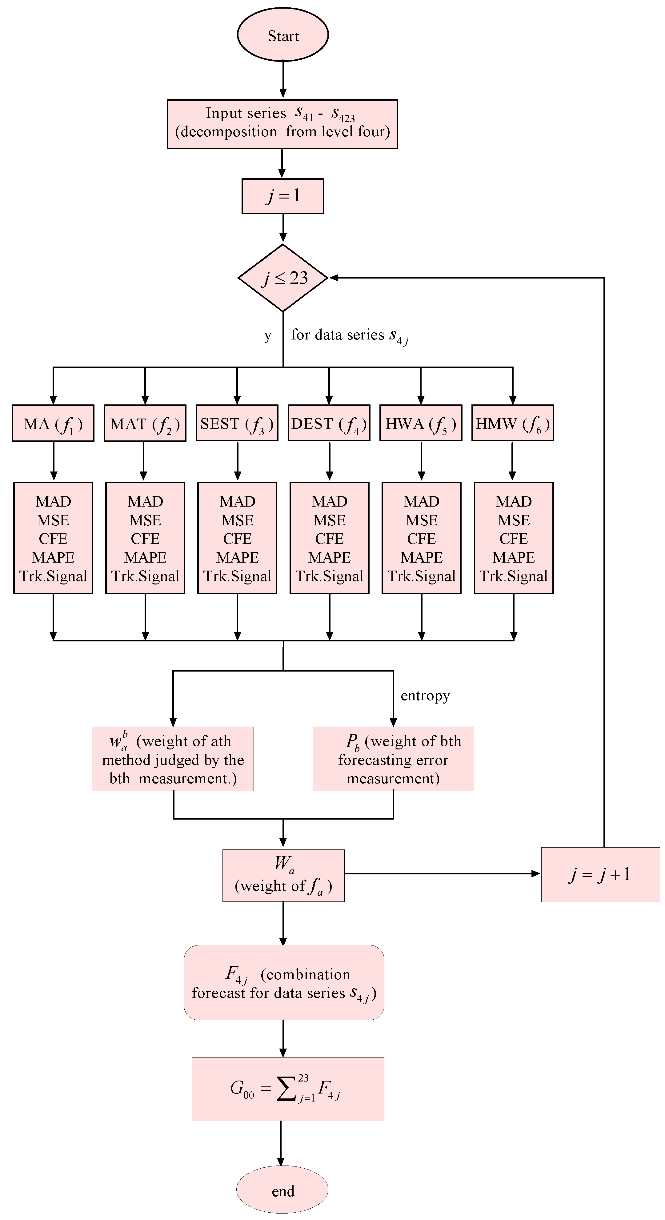
To explain the proposed method more clearly, a flow chart was developed, as shown in Figure 2 (decomposition-based CF at level four).

The analysis framework for the work was as follows:

Step 1: The total electricity demand ($s_{00}$) in the target society was decomposed into four industry levels (Figure 1), coded at level one to four: $s_{1j}$, $s_{2j}$, $s_{3j}$, $s_{4j}$ respectively (Table 1).

Step 2: For $s_{ij}$, ten time series groups were determined for each industry; $s_{ij}^1\sim s_{ij}^{10}$ (see the details in Section 3.1).

Step 3: For $s_{4j}^l$, the future electricity demand was forecast using the six individual models and CF. For $s_{3j}^l$, the future demand was forecast using the six individual models and CF and DCF4. For $s_{2j}^l$, the future demand was forecast using the six individual models and CF, DCF3, and DCF4. For $s_{1j}^l$, the future demand was forecast using the six individual models and CF, DCF2, DCF3, and DCF4. For $s_{00}^l$, the future demand was forecast using the six individual models and CF, DCF1, DCF2, DCF3, and DCF4.

Step 4: To compare and analyze the six individual models and the combination model for $s_{ij}$, an ANOVA and an orthogonal approach to solve the least squares equations were applied for which the AREs were regarded as the observation variables; therefore, there were 10 observations with 7 classification variables. For details, see Section 4.1 and Section 4.2).

Step 5: The decomposition-based CF models were compared and analyzed. For $s_{3j}$, an ANOVA and an orthogonal approach were applied for which the AREs were regarded as the observation variables; therefore, there were 10 observations and 8 independent variables, as shown in Section 4.3.1. For $s_{2j}$, an analysis of variance was applied for which there were 9 independent variables, as shown in Section 4.3.2. For $s_{1j}$, an analysis of variance was applied for which there were 10 independent variables, as shown in Section 4.3.3. For $s_{00}$, an analysis of variance was applied for which there were 11 independent variables, as shown in Section 4.3.4.

Step 6: To further substantiate the forecasting results for DCF4, a comparison analysis with other forecasting methods such as ARIMA and ANN was conducted, as shown in Section 4.4.

4. Results and Discussion

This section gives step-by-step comparison analyses for the individual models, the combination forecasting model, and the decomposition-based combination forecasting method.

4.1. Analysis of the Individual Methods

As both MAPE and MSE are average values, the outliers are also averaged, and therefore it is often difficult to detect the worst prediction and the forecasting stability. Therefore, to compare the impact and significance of the forecasting accuracy for each forecast method, in this section, an ANOVA was conducted with the comparison tests on ARE.

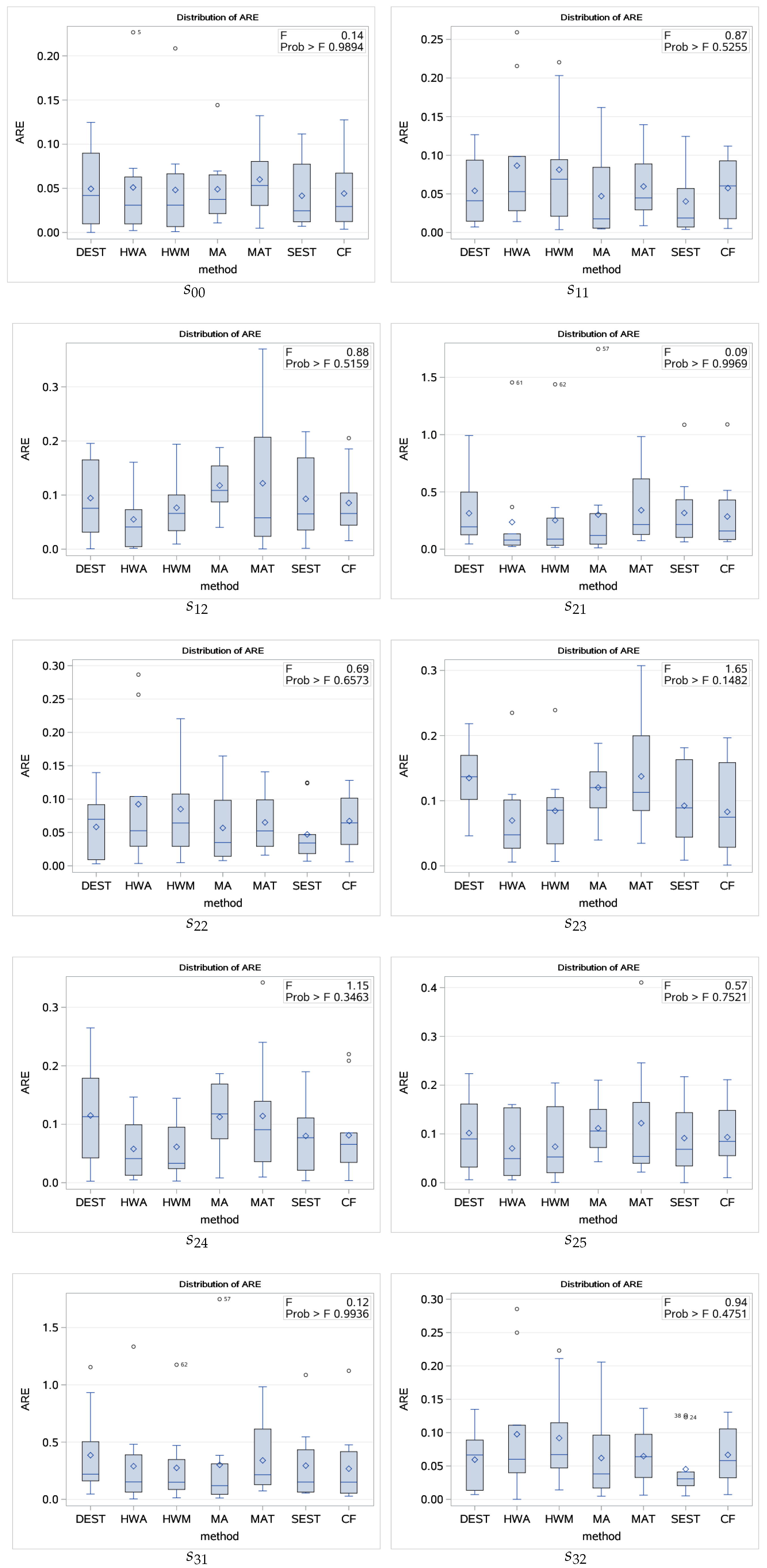
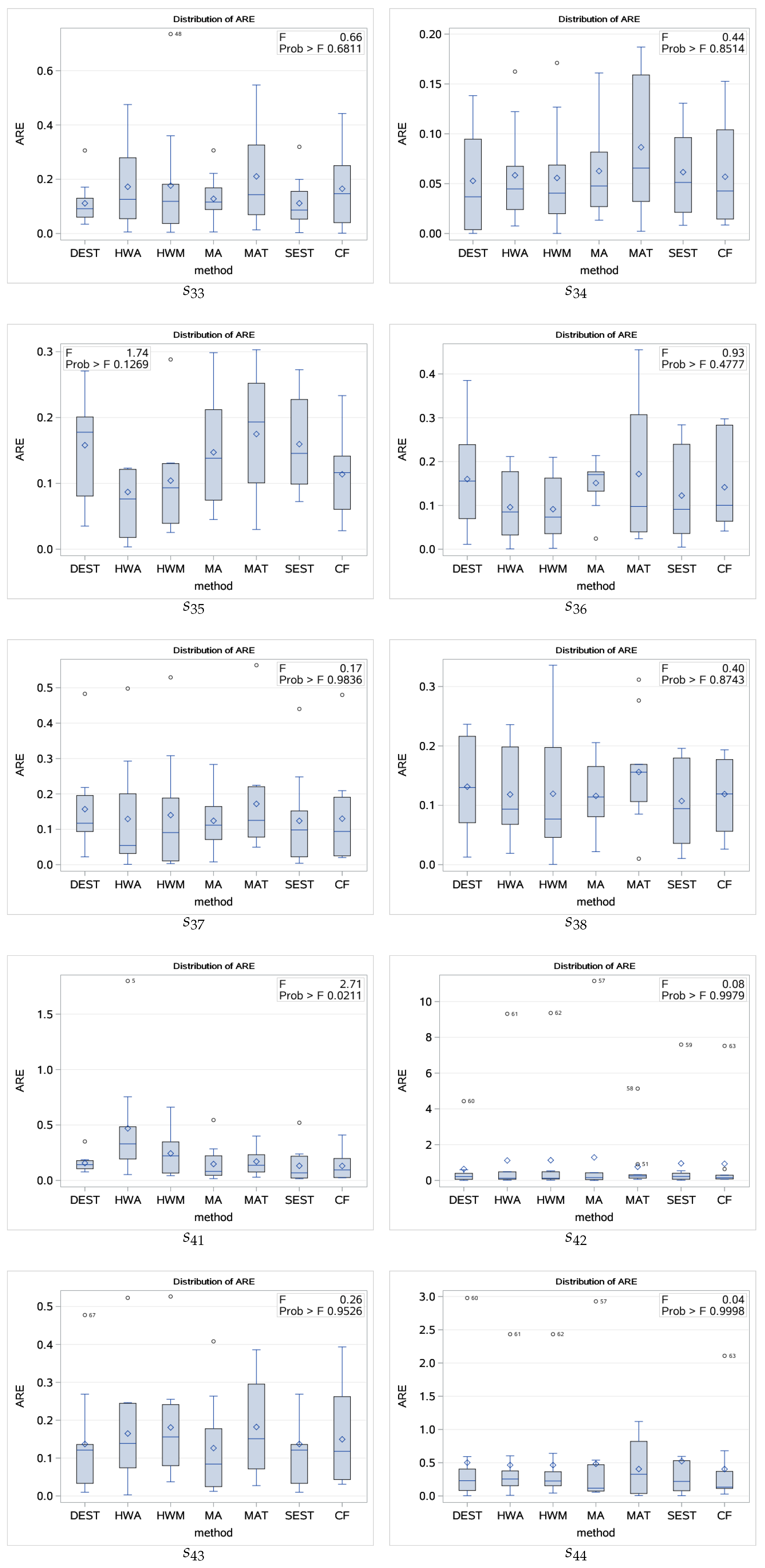
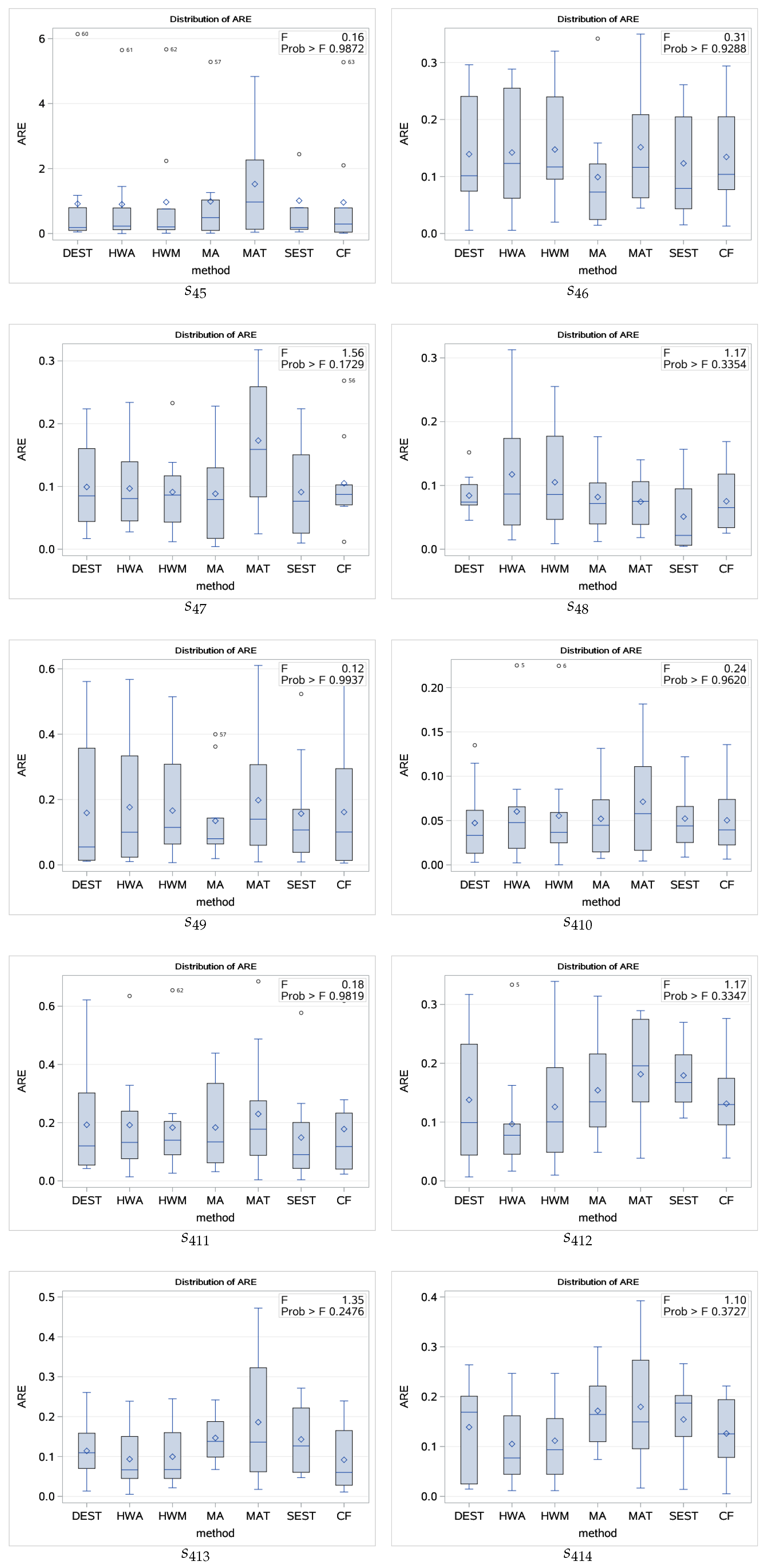
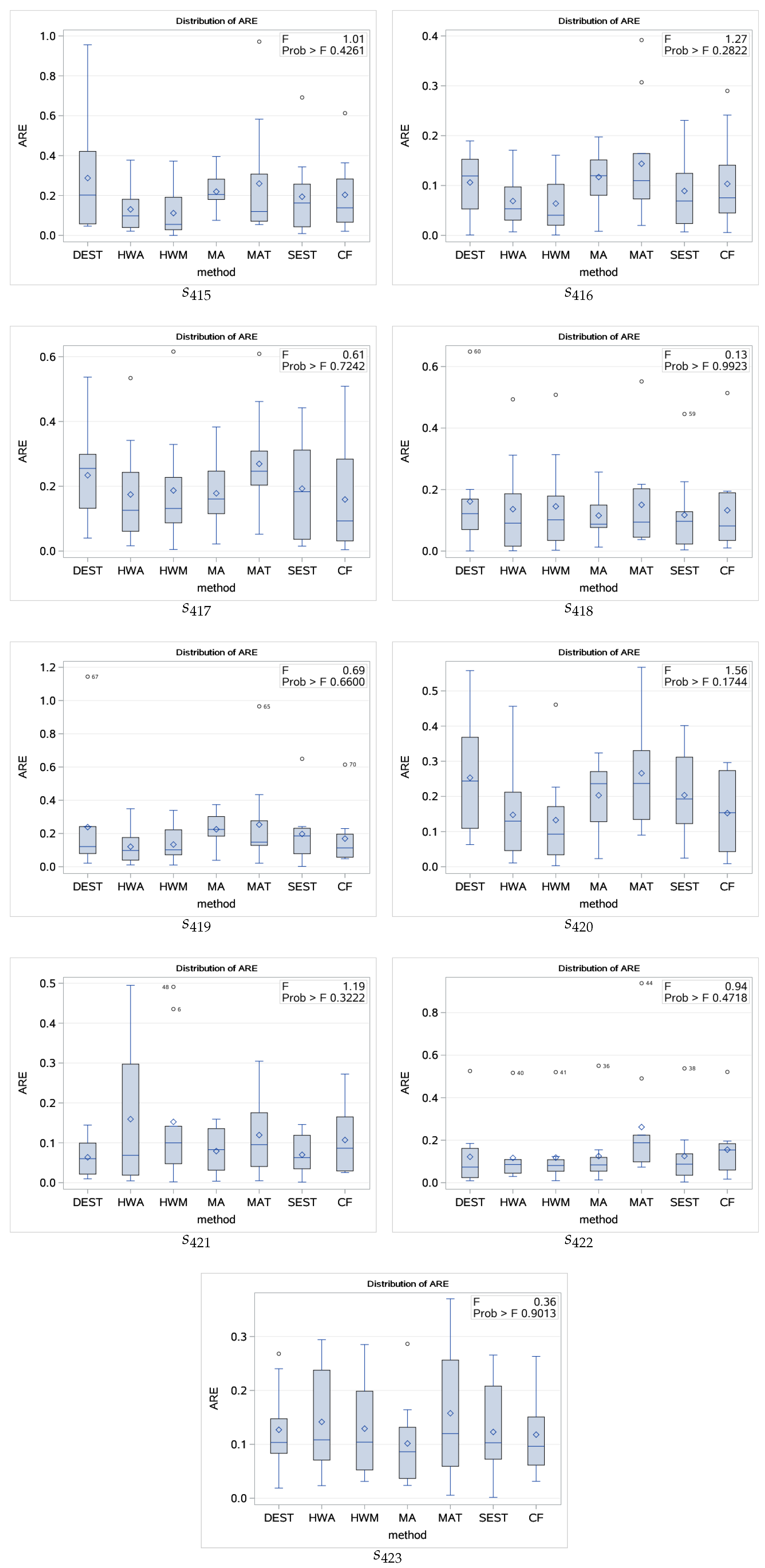
The forecasting error distribution (shown in Figure 3) was represented using schematic box-and-whisker plots, each of which contained forecast errors from the individual and the CF methods.

With the mean, median, Q1 (first quartile), Q3 (third quartile), and the outliers (more above $\mathrm{Q}3+1.5\ast \mathrm{IQR}$, where $\mathrm{IQR}=\mathrm{Q}3-\mathrm{Q}1$) as the comparison indicators, the adaptability of the individual methods was estimated, with the Q1, Median, and Q3 columns respectively providing the lower quantile, median, and upper quantile. The best, the second best, the worst, and the second worst individual methods for each industry are shown in

Table 3. Method adaptability for each industry.

Data	The Best	The Second Best	The Worst	The Second Worst	CF Rank	Unsuitable for the Data
$s_{00}$	SEST	DEST	HWA	HWM	2
$s_{11}$	SEST	DEST	HWA	HWM	4
$s_{12}$	HWA	HWM	WAT	SEST	3
$s_{21}$	HWA	HWM	MAT	DEST	3
$s_{22}$	SEST	DEST	HWA	HWM	5
$s_{23}$	HWA	HWM	MAT	DEST	3
$s_{24}$	HWA	HWM	MAT	DEST	4
$s_{25}$	HWA	HWM	MAT	DEST	4
$s_{31}$	MA	HWM	DEST	MAT	2	unsuitable
$s_{32}$	SEST	DEST	HWA	HWM	3
$s_{33}$	DEST	SEST	MAT	HWA	4
$s_{34}$	HWA	HWM	MAT	HWA	4
$s_{35}$	HWA	HWM	MAT	SEST	3
$s_{36}$	HWM	HWA	MAT	DEST	5
$s_{37}$	SEST	MA	MAT	DEST	3
$s_{38}$	SEST	MA	MAT	DEST	2
$s_{41}$	DEST	SEST	HWA	HWM	1
$s_{42}$	DEST	MAT	HWA	HWM	1	unsuitable
$s_{43}$	SEST	SEST	MAT	HWM	1
$s_{44}$	HWA	HWM	MAT	DEST	1
$s_{45}$	SEST	HWM	MAT	DEST	2	unsuitable
$s_{46}$	MA	SEST	HWM	HWA	3
$s_{47}$	MA	SEST	MAT	DEST	6
$s_{48}$	SEST	MA	HWA	HWM	4
$s_{49}$	SEST	MA	MAT	DEST	3
$s_{410}$	HWM	HWA	MAT	SEST	4
$s_{411}$	SEST	MA	MAT	DEST	2
$s_{412}$	HWA	HWM	MAT	DEST	2
$s_{413}$	HWA	HWM	MAT	MA	1
$s_{414}$	HWA	HWM	MAT	MA	3
$s_{415}$	HWM	HWA	DEST	MAT	4
$s_{416}$	HWM	HWA	MAT	MA	6
$s_{417}$	MA	SEST	MAT	DEST	1	unsuitable
$s_{418}$	SEST	MA	MAT	DEST	2
$s_{419}$	HWA	HWM	MAT	MA	3	unsuitable
$s_{420}$	HWM	HWA	MAT	DEST	1
$s_{421}$	DEST	SEST	HWA	HWM	4
$s_{422}$	HWA	HWM	MAT	DEST	5
$s_{423}$	MA	DEST	MAT	HWA	1

.

As can be seen in Figure 3, as the null hypothesis (same average estimates) was not able to be rejected at a 0.05 significance level, there were no major differences between the seven methods, which indicated that these classical time series forecasting methods could also be useful for forecasting electricity demand, which was consistent with the results in many previous studies. However, Figure 3 also indicates that MA also had good model fitness in some industries, and as the Q3 was lower than 10% and there were no outliers for $s_{11}$, $s_{22}$, $s_{32}$, $s_{34}$ and $s_{410}$, it also had a good forecasting performance. More importantly, an ARE lower than 10% is generally considered very satisfactory in engineering. Table 3 also shows that the MA had the best performance for $s_{31}$, $s_{46}$, $s_{417}$ and $s_{423}$ compared with the other individual methods. Unfortunately, MA also performed poorly; for $s_{41}$, $s_{413}$, $s_{414}$ and $s_{416}$ MA had the second worst performance compared with the other individual methods.

Karim and Alwi [31] concluded that the exponential smoothing technique had a better performance than the MA. Similarly, Figure 3 shows the effectiveness of SEST in some industries as the Q3 was lower than 0.1 and the ARE means were lower than 0.05 for $s_{00}$, $s_{11}$, $s_{22}$, $s_{32}$, $s_{48}$ and $s_{410}$. As shown in the first column of Table 3, SEST was the best individual method 11 times (28.2%) and MA was the best individual method five times (12.8%).

Figure 3 also shows that DEST was also an effective method and was able to perform well in some industries; the ARE means were lower than 0.05 for $s_{00}$, $s_{11}$, $s_{34}$, $s_{49}$ and $s_{410}$ and the Q3 was lower than 0.1 for $s_{00}$, $s_{11}$, $s_{22}$, $s_{32}$, $s_{34}$, $s_{410}$ and $s_{421}$. In addition, DEST had the best performance for $s_{33}$, $s_{41}$, $s_{42}$ and $s_{421}$ compared to the other individual methods.

Hussain et al. [5] proved that the Holt-Winters forecasting model could have robust results, and as shown in Table 3, this model outperformed some other methods in some industries. The MA, MAT, SEST, DEST, HWA and HWM models were respectively identified as the best individual methods five times (12.8%), zero times(0%), 11 times (28.2%), four times (10.3%), 14 times (35.9%) and five times (12.8%), with the HWA, and HWM together accounting for 49.2%. The MA, MAT, SEST, DEST, HWA, and HWM were respectively identified as the second best individual methods six times(15.4%), one time (2.6%), six times (15.4%), six times (15.4%), five times (12.8%) and 15 times (38.5%), the HWA and HWM together accounting for 51.3%. These results demonstrated that the Holt-Winters forecasting method outperformed the other individual methods in most cases.

However, it is somewhat difficult to explore the effectiveness and superiority of the Holt-Winters forecasting method as special attention needs to be paid to accuracy. In some cases, none of the methods was found to be suitable. As shown in Figure 3 and Table 3, however, for most of the rest, the Holt–Winters forecasting method produced accurate results, with the Q3 being lower than 0.1 and the median and means being lower than 0.05.

However, a further analysis of Figure 3 and Table 3 indicated that HWA and HWM were the worst individual methods eight times (20.5%) and one time (2.6%), and the second worst individual methods four times (10.25%) and nine times (23.1%). Therefore, as the Holt-Winters forecasting method was not available for all the time series data, it could be unhelpful for electricity demand forecasting in some industries.

From these analyses, it was concluded that as there was no one technique that was able to always obtain better forecasting results, different time series data sets require different individual methods. Therefore, there is no best forecasting model for the electricity data sets from different industries.

4.2. Analysis of the Combination Forecasting Model

In the combination forecasting model proposed in this paper, inverse error weights were used so that the individual methods with less errors received an increased weight; that is, the advantages of each individual method were combined to improve the forecasting accuracy. Figure 3 shows that the CF had excellent forecasting performance as the Q3 was lower than 0.1 for $s_{00}$, $s_{11}$, $s_{12}$, $s_{22}$, $s_{410}$ and the median was lower than 0.05 for $s_{00}$, $s_{34}$ and $s_{410}$.

Column 6 in Table 3 shows the CF Rank for the combination forecasting model compared to the other seven forecasting methods for each different industry. The CF model was respectively ranked from one to eight, 8, 7, 10, 9, 2, 3, and 0 times; that is, the combination forecasting method ranked in the top three 74.9% of the time, indicating its overall effectiveness. These results clearly indicated that forecasting combinations can yield unbiased forecasts even if the individual forecasts are biased. However, a more in-depth analysis of Figure 3 indicated that there were some industries in which none of the methods (including the combination model) were useful; $s_{31}$, $s_{45}$, $s_{417}$, $s_{419}$, $s_{422}$.

To determine the reason for this, the original electricity data from each industry were reanalyzed, from which it was found that there was a large gap between September 2009 and the other months in most industries. Therefore, it was concluded that a combination approach was not suitable when the data were highly volatile.

4.3. Comparison Analysis of the Decomposition Experiments

To demonstrate the decomposition-based CF method, in this section, an ANOVA was used to analyze the electricity demand forecasting at the sub-subsector levels, the sub-sector levels, the sector levels, and the total aggregate level.

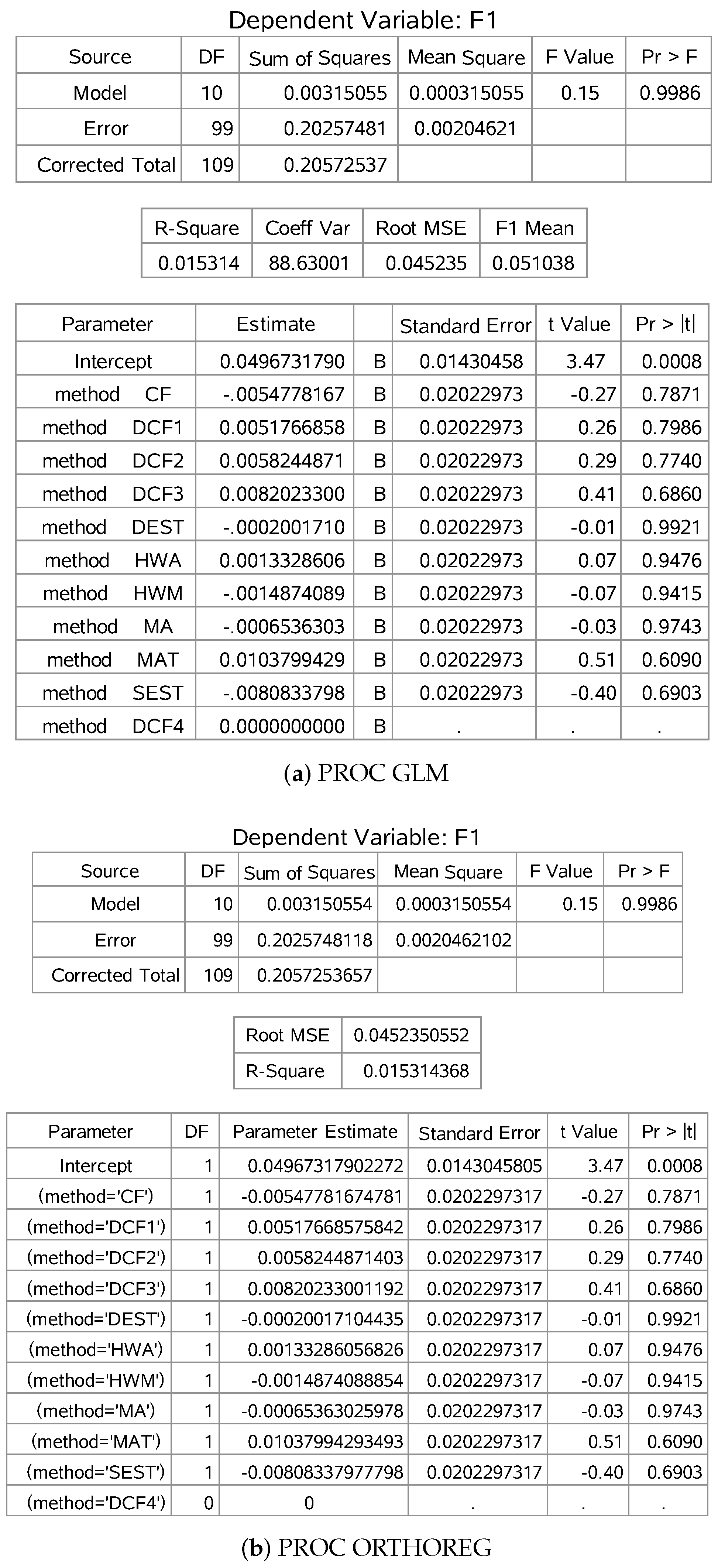
In the ANOVA, the ‘B’ following the parameter estimates indicated that the estimates were biased and did not represent a unique solution to the normal equations (Figure 4a). However, when using the orthogonal approach (ORTHOREG) to solve the least squares equations, more accurate estimates were produced compared to the other regression procedures. Figure 4b shows that the ORTHOREG fit achieved the same root mean square error (RMSE) as shown in the ANOVA table but avoided the spurious singularities; therefore, the following analyses only considered the ANOVA. Furthermore, while there were no significant differences between DCF4 and the other methods when the other methods were superior to DCF4 in all situations, there were significant differences between DCF4 and other methods when DCF4 was superior to other methods in some situations. Figure 5a,b shows that the differences between DCF4 and the MAT groups (for $s_{23}$) were marginal (p = 0.0959), and that the differences between DCF4 and the MAT (for $s_{35}$) were marginally significant (p = 0.0402), which indicated that DCF4 may be more effective. A detailed analysis was then conducted, as outlined in the following.

4.3.1. Forecasting for the Sub-Subsector Electricity Demand

Based on Equation (2), the sub-subsector electricity demand was forecast using a decomposition-based CF at level 4.

$${\displaystyle G_{3j}^4=\sum _v{F}_{4v},j=1,\cdots ,8,}$$

where $G_{3j}^4$ was the forecast for industry $s_{3j}$ using the decomposition-based CF at level 4 and $F_{4v}$ was the forecast for industry $s_{4v}$ using the combination forecasting model. For example, the forecast using DCF4 for industry $s_{31}$ was $G_{31}^4=F_{41}+F_{42}+F_{43}+F_{44}+F_{45}$.

The ARE outputs using the eight methods at the sub-subsector level were compared using ANOVA, and the forecasting error distribution is shown in Figure 6. Figure 1 shows that there was no branch industry for $s_{33}$, indicating that no DCF4 existed for $s_{33}-\mathrm{plus}$. The distribution of the forecast errors in Figure 6 shows the data discrepancy and biases as well as the outliers. For $s_{32}-\mathrm{plus}$, DCF4 achieved the lowest ARE means compared to all other methods except SEST; however, SEST had two outliers. DCF4 also achieved the lowest median except for SEST and MA, but MA had an internal cap that was far greater than for the DCF4. More importantly, 75% of the DCF4 AREs were lower than 10%, which was considered satisfactory.

For $s_{38}-\mathrm{plus}$, DCF4 had the best forecasting performance as it achieved the lowest ARE means, Q1 and Q3, and had no outliers. For s34-plus, the DCF4 had the third best performance after MA and DEST, as it achieved the lowest Q1 and means, and there were no outliers.

Even though all methods appeared to be unhelpful for industry $s_{35}$, DCF4 achieved the lowest means. However, no methods were suitable for the data associated with $s_{31}-\mathrm{plus}$, $s_{35}-\mathrm{plus}$, $s_{36}-\mathrm{plus}$ and $s_{37}-\mathrm{plus}$. An analysis of the original electricity data indicated that there was a big gap between September 2009 and the other months in most industries.

From the above, it can be concluded that the forecasting effect tends to be better after adopting decomposition; however, a DCF with only one decomposition level is sometimes not suitable when the data are highly volatile

4.3.2. Forecasting for the Sub-Sector Electricity Demand

Based on Equation (2), the sub-sector electricity demand was forecast using the decomposition–based CF at levels 4 and 3 using the following formula;

$${\displaystyle G_{2j}^4=\sum _v{F}_{4v},j=1,\cdots ,5,G_{2j}^3=\sum _v{F}_{3v},j=1,\cdots ,5,}$$

where $G_{2j}^4$ and $G_{2j}^3$ were respectively the forecasts for industry $s_{2j}$ using the decomposition-based CF at levels 4 and 3, and $F_{4v}$ and $F_{3v}$ were the forecasts for industry $s_{4v}$ and $s_{3v}$ using the combination forecasting model.

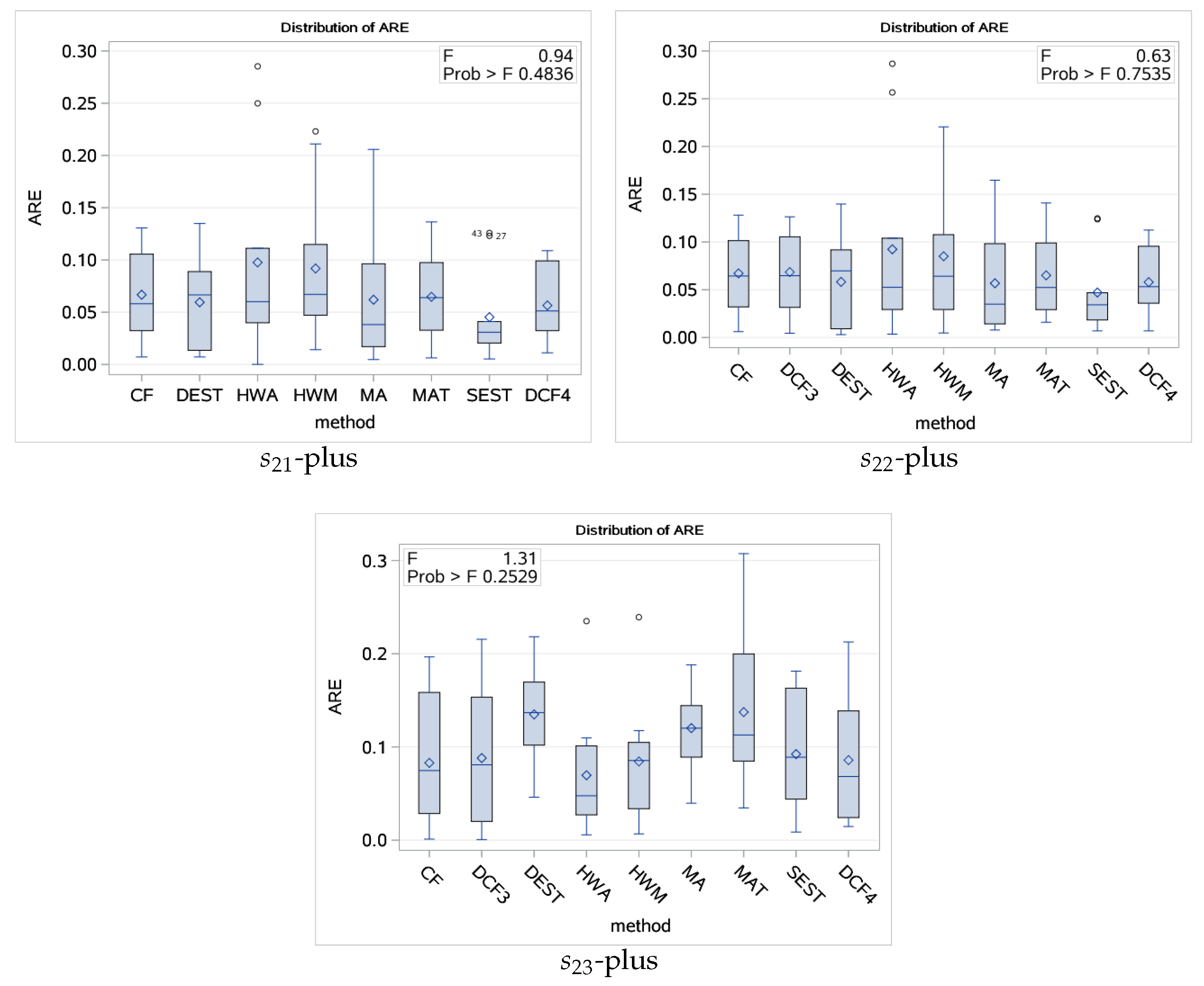
Figure 7 compares the differences in the ARE output distributions for the nine sub-sector methods. From Figure 7, it can be seen that DCF4 achieved the lowest ARE means (approximately 0.05) compared to all other methods except for SEST, which had outliers in $s_{22}-\mathrm{plus}$, 75% of the ARE outputs from DCF4 were lower than 10%, and DCF4 also had the lowest median, means and Q3 and no outliers compared to all other methods except for HWA and HWM, both of which have an outlier in $s_{23}-\mathrm{plus}$. No methods, however, were found to be suitable for $s_{21}$. These results demonstrated that electricity demand forecasting uncertainties can be reduced using decomposition.

4.3.3. Forecasting for Sector Demand

Based on Equation (2), the sector electricity demand was forecast using a decomposition-based CF at levels 4, 3 and 2:

$$\begin{array}{cc}\hfill G_{1j}^4& {\displaystyle =\sum _v{F}_{4v},j=1,2,G_{1j}^3=\sum _v{F}_{3v},j=1,2,}\hfill \\ \hfill G_{1j}^2& {\displaystyle =\sum _v{F}_{2v},j=1,2,}\hfill \end{array}$$

where $G_{2j}^4$, $G_{2j}^3$ and $G_{2j}^1$ were the respective forecasts for industry $s_{1j}$ using DCF4, DCF3, and DCF2 respectively, and $F_{4v}$, $F_{3v}$ and $F_{2v}$ were the forecasts for industry $s_{4v}$, $s_{3v}$ and $s_{2v}$ using the combination forecasting model.

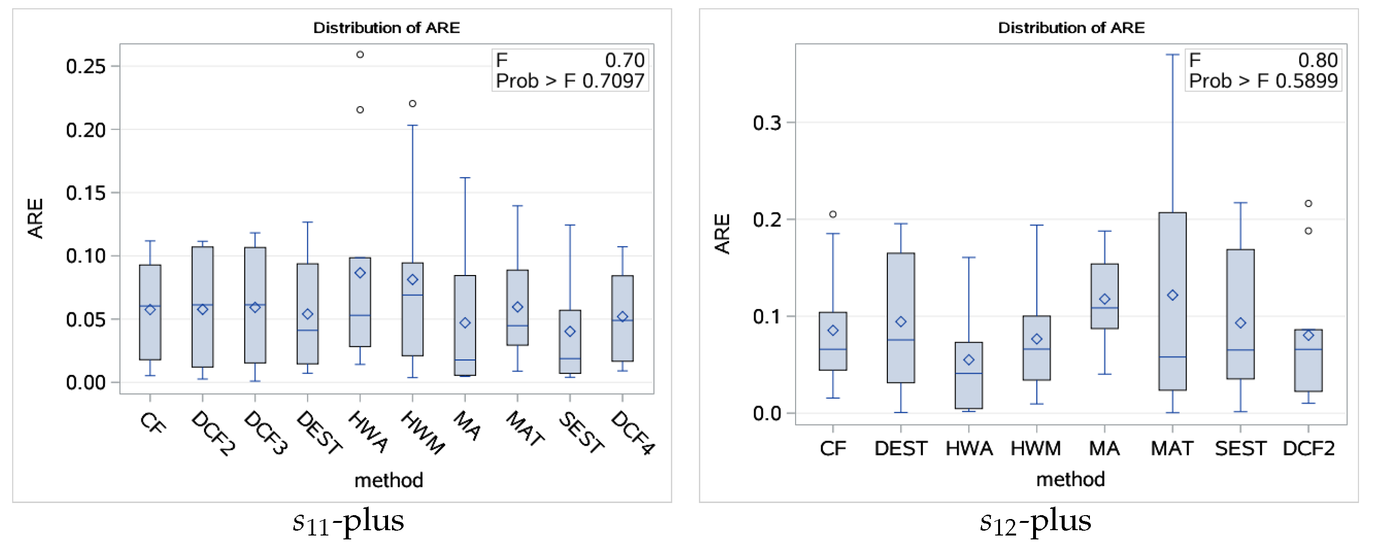
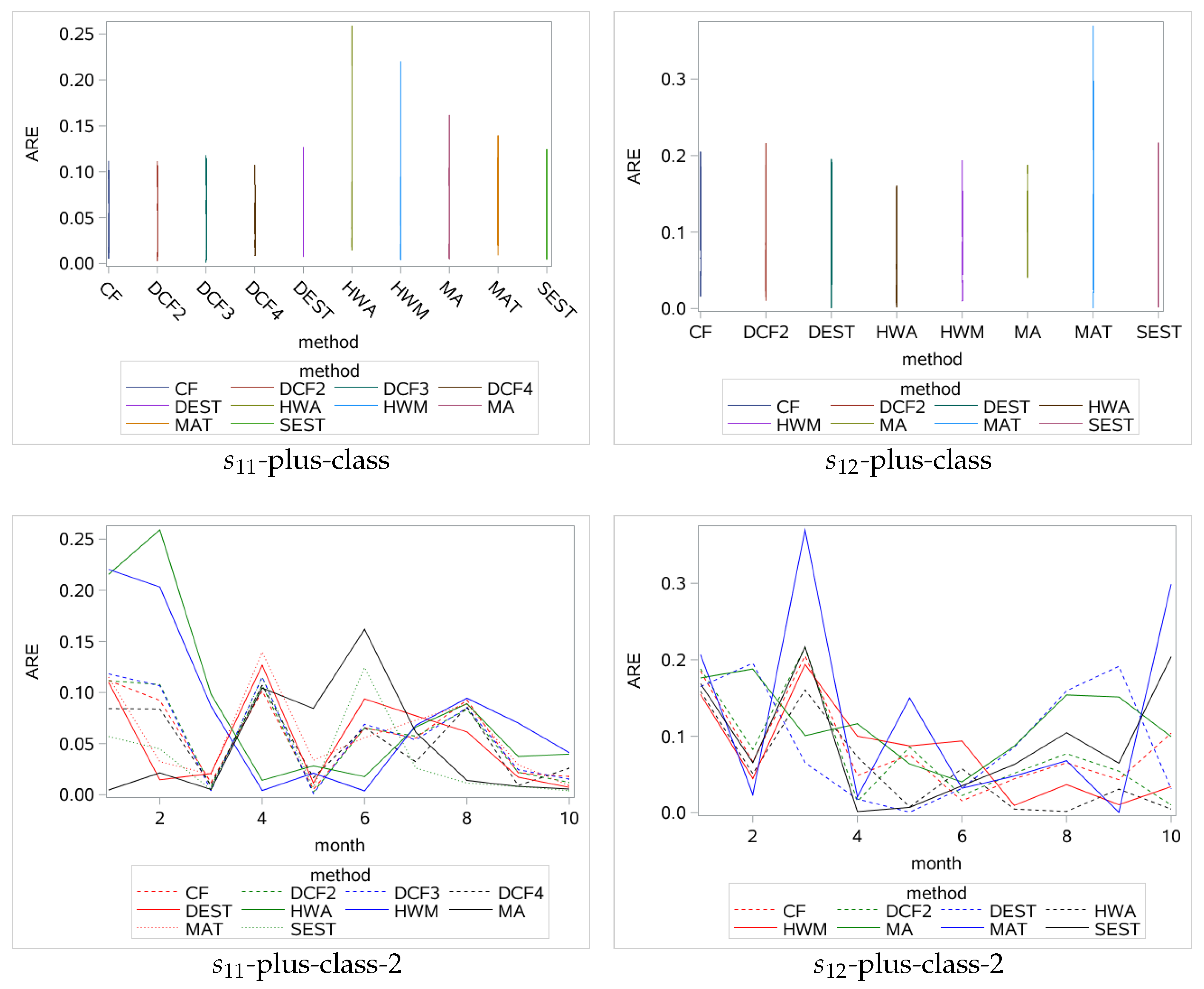
The ARE outputs for sector demand for the ten methods were compared using ANOVA, and the forecasting error distributions together with the schematic box-and-whisker plot representations are shown in Figure 8. $s_{12}$ was residential electricity and was only decomposed from level 2 without DCF3 and DCF4, and $s_{11}$ was decomposed from level 2 through to level 4.

A comparison in Figure 9 clearly shows that the decomposition-based CF model had the best forecasting performance for $s_{11}$, which was decomposed from three levels; however, the decomposition-based combination forecasting model had no advantages when forecasting $s_{12}$ as there was only one decomposition level. DCF4 had the smallest maximum error when forecasting $s_{11}$, and DCF2 had a similar inner fence to the other methods. These results demonstrated that decomposition can adapt to the various characteristics of different data series.

Although Figure 8 indicates that HWA had the best performance for $s_{12}-\mathrm{plus}$ (which was consistent with the forecasting results in Hussain et al. [5]), for $s_{11}-\mathrm{plus}$, both HWA and HWM had outliers, indicating that these methods were not suitable for the data set. In this case, for $s_{11}-\mathrm{plus}$, DCF4 achieved the best performance because it had the lowest Q3 and means, the narrowest inner fence, and no high Q1 compared with all other methods except for SEST. Figure 9 also shows that DCF4 had smaller volatility than SEST.

4.3.4. Forecasting for Total Electricity Demand

Governments are most interested in total electricity demand forecasting as this allows them to make future plans. Based on Equation (2), the electricity demand was forecast using the decomposition–based combination method described in Section 3.5.

Figure 10 shows that when only considering the means, the CF and SEST methods achieved better performance and the MAT and DCF3 methods had the worst performance. When considering the outliers, the CF, DCF4 and SEST methods achieved better performance, and the HWA, HWM, and MA methods contained outliers. For the degree of dispersion, the DCF4 achieved a lower $\mathrm{Q}1-1.5\ast \mathrm{IQR}$ and a lower $\mathrm{Q}3+1.5\ast \mathrm{IQR}$, followed by SEST, CF, DCF1, DCF2. These results further supported the conclusion that decomposition-based combination forecasting at level 4 is better at forecasting total electricity demand.

At any time, actual power generation must be able to accommodate at least a 15% increase in demand [32]. Figure 11a shows that even though the data are complex and uncertain, DCF4 performed excellently as all the AREs were lower than 10%. Figure 11b also shows that with an increase in the learning period, the decomposition-based combination forecasting model errors tended to decrease, and the DCF4 remained more stable under volatility compared with the other methods. Furthermore, as can be seen from the ARE outputs for all methods for $s_{00}$ in

Table 4. The AREs of all the methods for $s_{00}$.

Month	MA	MAT	SEST	DEST	HWA	HWM	CF	DCF1	DCF2	DCF3	DCF4
25	0.0367	0.1323	0.0774	0.1246	0.2266	0.2084	0.1276	0.1255	0.1258	0.1312	0.1036
26	0.0214	0.0306	0.0223	0.0004	0.0727	0.0665	0.0124	0.0870	0.1027	0.1018	0.0837
27	0.0218	0.0805	0.0337	0.0322	0.0098	0.0067	0.0321	0.0454	0.0313	0.0343	0.0301
28	0.0697	0.1209	0.0969	0.1033	0.0370	0.0297	0.0957	0.0932	0.0926	0.0995	0.0927
29	0.0611	0.0048	0.0071	0.0001	0.0088	0.0091	0.0091	0.0075	0.0113	0.0143	0.0275
30	0.1442	0.0525	0.1115	0.0898	0.0243	0.0049	0.0672	0.0581	0.0590	0.0623	0.0595
31	0.0652	0.0540	0.0122	0.0505	0.0249	0.0323	0.0267	0.0398	0.0403	0.0371	0.0191
32	0.0383	0.0616	0.0090	0.0351	0.0629	0.0775	0.0480	0.0654	0.0556	0.0570	0.0578
33	0.0209	0.0239	0.0190	0.0098	0.0022	0.0010	0.0038	0.0253	0.0278	0.0299	0.0025
34	0.0109	0.0394	0.0269	0.0487	0.0409	0.0456	0.0193	0.0013	0.0086	0.0113	0.0203

, there were more minimum AREs for the DCF4 model than for the other models. Even though they had fewer errors sometimes, the individual methods tended to display some instability, with errors ranging from very small to high; for example, the HWA had forecasting errors for $s_{00}$ that were close to zero but as high as 20%. By default, compared to “accuracy”, stability is particularly important for engineering practice.

4.4. Comparison Analysis with Benchmark Methods

To further substantiate the forecasting results for DCF4, a comparison analysis was conducted with the benchmark methods ARIMA and ANN, both of which have been proven to be effective and highly precise [1,33]. For the comparison, the total electricity demand ($s_{00}$) forecasting was executed by ARIMA and ANN.

The basic steps for ARIMA were as follows. First, the nonstationary series were transformed to stationary series using differencing, after which p (the order of the autoregressive part) and q (the order of the moving-average process) were determined using ACF and PACF and the optimal model determined from the check of the white noise residuals.

Three months’ worth of electricity consumption data before the month to be predicted were taken as the input data for the ANN model, which had three input neurons. The number of hidden neurons were arranged to take values between 2 and 10, with the one output neuron being the consumption forecast for the subsequent month, and the leave-one-out cross-validation method used to evaluate the model. In addition, a rectified linear unit activation function was used as the hidden layer activation function, a linear function was used in the output layer, and an adaptive moment estimation was employed as the learning algorithm.

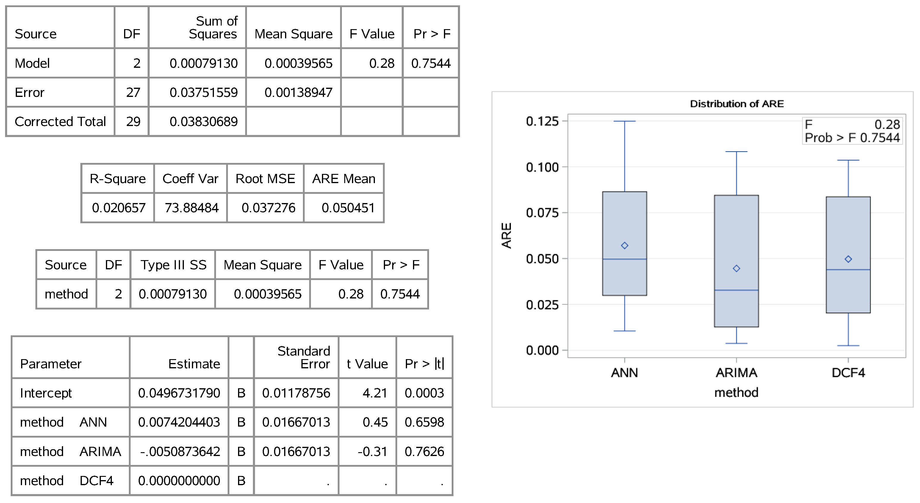
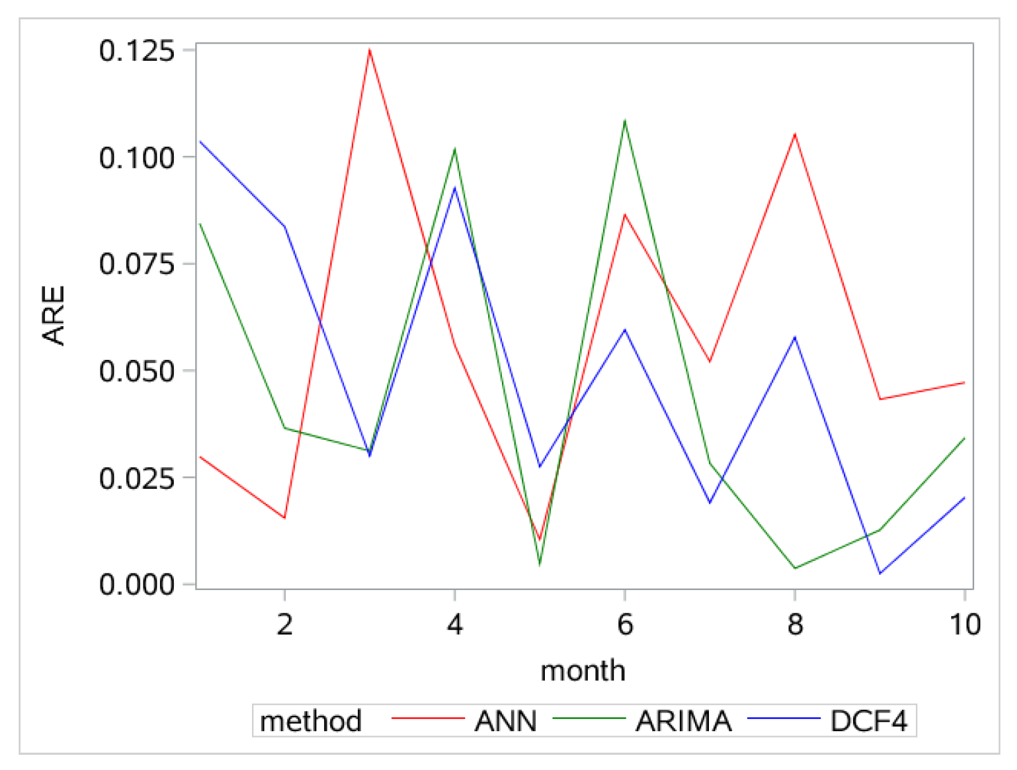
The analysis of variance results in Figure 12 indicated that there were no significant differences between the ANN, ARIMA, and DCF4 (p = 0.7544). However, both

Table 5. The AREs of the ANN, ARIMA, and DCF4 for $s_{00}$.

Month	ANN	ARIMA	DCF4
25	0.029848707	0.084465171	0.103625946
26	0.015499663	0.036508881	0.083654997
27	0.124882225	0.031200544	0.030069406
28	0.055943052	0.101710947	0.092687115
29	0.010492949	0.004772692	0.027535572
30	0.086425693	0.108288557	0.059520543
31	0.052094060	0.028256914	0.019058591
32	0.105269199	0.00370881	0.057769253
33	0.043279300	0.01268148	0.002516652
34	0.047201343	0.034264153	0.020293710

and Figure 13 show that the DCF4, ARIMA, and ANN forecasting results agreed. The ARE outputs for the ANN, ARIMA, and DCF4 in Table 5 indicated that there were more minimum AREs for the DCF4 model than for either the ARIMA or ANN models, and that all the DCF4 errors were lower than 0.01 and tended to decrease with an increase in the learning period, as shown in Figure 13, all of which illustrated that the DCF4 was more stable, even when there was not enough data.

5. Conclusions

With a focus on both prediction accuracy and stability, this paper developed a method for total electricity demand forecasting for nonlinear, nonstationary series. Using dynamic adaptive entropy-based weighting, a dynamic adaptive model was developed for total electricity demand forecasting that could be dynamically adapted to various forecast models through combination and to the various data characteristics through decomposition.

In this work, the total electricity demand in the target society was first decomposed based on industry categories, after which each component was forecast using a combination model that was developed using the entropy method, from which it was found that decomposition together with combination forecasting was able to improve forecasting accuracy.

The analyses of the individual methods in specific environments found that HWA was suitable for most data sets due to its varied applications; however, no significant differences were found between the forecast models based on the ANOVA. DCF4 was found to perform better than either the ARIMA or the ANN, especially when there was only small data and no need to handle outliers. From the schematic box-and-whisker plots and with the means, median, Q1, Q3, and outliers as the comparison indicators, it was found that the dynamic adaptive forecasting model performed the best, was highly accurate, had formidable forecasting ability, and would therefore be the best choice for complex, variable data. It was also concluded that if the raw data outliers were omitted, all methods analyzed here would perform better. It was also found that the large gap between September 2009 and the other months for most industries significantly affected the forecasting.

Although this paper was focused on the forecasting of monthly series data sets, the methods shown here could also be applied to quarterly data. As the proposed model performed well in forecasting one period, it could be used to develop electricity generation plans and associated energy policies. To further improve the methods, the forecast periods could be extended, and classical forecasting models and modern intelligent forecasting models combined to develop combination models for every industry; therefore, more work is necessary to fully refine the methodology.

References

1. Laouafi, A.; Mordjaoui, M.; Haddad, S.; Boukelia, T.E.; Ganouche, A. Online electricity demand forecasting based on an effective forecast combination methodology. Electr. Power Syst. Res. 2017, 148, 35–47. [Google Scholar] [CrossRef]
2. Rallapalli, S.R.; Ghosh, S. Forecasting monthly peak demand of electricity in India-A critique. Energy Policy 2012, 45, 516–520. [Google Scholar] [CrossRef]
3. Hongye Guo, Q.C.; Qing Xia, C.K.; Zhang, X. A monthly electricity consumption forecasting method based on vector error correction model and self-adaptive screening method. Int. J. Electr. Power Energy Syst. 2018, 95, 427–439. [Google Scholar]
4. Li, W.; Yang, X.; Li, H.; Su, L. Hybrid Forecasting Approach Based on GRNN Neural Network and SVR Machine for Electricity Demand Forecasting. Energies 2017, 10, 44. [Google Scholar] [CrossRef]
5. Hussain, A.; Rahman, M.; Memon, J.A. Forecasting electricity consumption in Pakistan: The way forward. Energy Policy 2016, 90, 73–80. [Google Scholar] [CrossRef]
6. Li, W.; Bao, Z.; Huang, G.H.; Xie, Y.L. An Inexact Credibility Chance-Constrained Integer Programming for Greenhouse Gas Mitigation Management in Regional Electric Power System under Uncertainty. J. Environ. Inform. 2018, 31, 111–122. [Google Scholar] [CrossRef]
7. Brown, R.G. Exponential Smoothing. Encycl. Oper. Res. Manag. Sci. 2013, 11, 537–539. [Google Scholar] [CrossRef]
8. Box, G.E.P.; Tiao, G.C. Intervention Analysis with Applications to Economic and Environmental Problems. Publ. Am. Stat. Assoc. 1975, 70, 70–79. [Google Scholar] [CrossRef]
9. Akaike, H. Canonical Correlation Analysis of Time Series and the Use of an Information Criterion. Math. Sci. Eng. 1976, 126, 27–96. [Google Scholar] [CrossRef]
10. Kumar, U.; Jain, V.K. Time series models (Grey-Markov, Grey Model with rolling mechanism and singular spectrum analysis) to forecast energy consumption in India. Energy 2010, 35, 1709–1716. [Google Scholar] [CrossRef]
11. Braun, M.R.; Altan, H.; Beck, S.B.M. Using regression analysis to predict the future energy consumption of a supermarket in the UK. Appl. Energy 2014, 130, 305–313. [Google Scholar] [CrossRef] [Green Version]
12. Khotanzad, A.; Hwang, R.C.; Abaye, A.; Maratukulam, D. An adaptive modular artificial neural network hourly load forecaster and its implementation at electric utilities. IEEE Trans. Power Syst. 1995, 10, 1716–1722. [Google Scholar] [CrossRef]
13. Son, H.; Kim, C. Short-term forecasting of electricity demand for the residential sector using weather and social variables. Resour. Conserv. Recycl. 2015, 123, 200–207. [Google Scholar] [CrossRef]
14. Van der Meer, D.; Shepero, M.; Svensson, A.; Widén, J.; Munkhammar, J. Probabilistic forecasting of electricity consumption, photovoltaic power generation and net demand of an individual building using Gaussian Processes. Appl. Energy 2018, 213, 195–207. [Google Scholar] [CrossRef]
15. Burger, E.M.; Moura, S.J. Gated ensemble learning method for demand-side electricity load forecasting. Energy Build. 2015, 109, 23–34. [Google Scholar] [CrossRef]
16. Clemen, R.T. Combining forecasts: A review and annotated bibliography. Int. J. Forecast. 1989, 5, 559–583. [Google Scholar] [CrossRef]
17. Xiao, L.; Shao, W.; Yu, M.; Ma, J.; Jin, C. Research and application of a combined model based on multi-objective optimization for electrical load forecasting. Energy 2017, 119, 1057–1074. [Google Scholar] [CrossRef]
18. Li, S.; Goel, L.; Wang, P. An ensemble approach for short-term load forecasting by extreme learning machine. Appl. Energy 2016, 170, 22–29. [Google Scholar] [CrossRef]
19. Wang, J.; Zhu, W.; Zhang, W.; Sun, D. A trend fixed on firstly and seasonal adjustment model combined with the -SVR for short-term forecasting of electricity demand. Energy Policy 2009, 37, 4901–4909. [Google Scholar] [CrossRef]
20. Shao, Z.; Chao, F.; Yang, S.L.; Zhou, K.L. A review of the decomposition methodology for extracting and identifying the fluctuation characteristics in electricity demand forecasting. Renew. Sustain. Energy Rev. 2017, 75, 123–136. [Google Scholar] [CrossRef]
21. Zhang, J.; Wei, Y.; Li, D.; Tan, Z.; Zhou, J. Short term electricity load forecasting using a hybrid model. Energy 2018, 158, 774–781. [Google Scholar] [CrossRef]
22. Li, C.; Tao, Y.; Ao, W.; Yang, S.; Bai, Y. Improving forecasting accuracy of daily enterprise electricity consumption using a random forest based on ensemble empirical mode decomposition. Energy 2018, 165, 1220–1227. [Google Scholar] [CrossRef]
23. Chen, J.S.; Chen, W.G.; Sun, P. A Generalized Model for Wind Turbine Faulty Condition Detection Using Combination Prediction Approach and Information Entropy. J. Environ. Inform. 2018, 32, 14–24. [Google Scholar] [CrossRef]
24. Che, J.X.; Wang, J.Z. Short-term load forecasting using a kernel-based support vector regression combination model. Appl. Energy 2014, 132, 602–609. [Google Scholar] [CrossRef]
25. Tang, P.; Chen, D.; Hou, Y. Entropy method combined with extreme learning machine method for the short-term photovoltaic power generation forecasting. Chaos Solitons Fractals 2016, 89, 243–248. [Google Scholar] [CrossRef]
26. Holt, C. Forecasting Trends and Seasonal by Exponentially Weighted Averages; Office of Naval Research Memorandum: Seattle, WA, USA, 1957. [Google Scholar]
27. Gooijer, J.G.D.; Hyndman, R.J. 25 years of time series forecasting. Int. J. Forecast. 2006, 22, 443–473. [Google Scholar] [CrossRef] [Green Version]
28. Gelper, S.; Fried, R.; Croux, C. Robust forecasting with exponential and Holt-Winters smoothing. J. Forecast. 2007, 29, 285–300. [Google Scholar] [CrossRef]
29. Anderson, D.R.; Sweeney, D.J.; Williams, T.A.; Camm, J.D.; Martin, R.K. An Introduction to Management Science: Quantitative Approaches to Decision Making; West Pub. Co.: New York, NY, USA, 1994; p. 128. [Google Scholar]
30. San-Juan, J.F.; San-Martín, M.; Pérez, I.; López, R. Hybrid perturbation methods based on statistical time series models. Adv. Space Res. 2015, 57, 1641–1651. [Google Scholar] [CrossRef]
31. Karim, S.A.A.; Alwi, S.A. Electricity load forecasting in UTP using moving averages and exponential smoothing techniques. Appl. Math. Sci. 2013, 7, 4003–4014. [Google Scholar] [CrossRef]
32. Williams, H.P. Model Building in Mathematical Programming. News Med. 2013, 264, 1132–1138. [Google Scholar]
33. Hamzaçebi, C. Forecasting of Turkey’s net electricity energy consumption on sectoral bases. Energy Policy 2007, 35, 2009–2016. [Google Scholar] [CrossRef]
Figure 1. Electricity decomposition.
Sustainability 11 01272 g001
Figure 2. The Flow chart for the dynamic adaptive forecasting process.
Sustainability 11 01272 g002
Figure 3. ARE distribution by ANOVA for every industry electricity demand.
Sustainability 11 01272 g003aSustainability 11 01272 g003bSustainability 11 01272 g003cSustainability 11 01272 g003d
Figure 4. The GLM procedure and the ORTHOREG procedure for s00.
Sustainability 11 01272 g004
Figure 5. Parameter Estimate.
Sustainability 11 01272 g005
Figure 6. ARE distribution by ANOVA for sub-sector electricity demand.
Sustainability 11 01272 g006
Figure 7. ARE distribution by ANOVA for sector.
Sustainability 11 01272 g007
Figure 8. ARE distribution by ANOVA for the sectors electricity demand.
Sustainability 11 01272 g008
Figure 9. Sorted Data with Contrast Colors and Line Patterns Specified for s11 and s12.
Sustainability 11 01272 g009
Figure 10. ARE distribution of by ANOVA for total electricity demand.
Sustainability 11 01272 g010
Figure 11. Sorted Data with Contrast Colors and Line Patterns Specified for s00.
Sustainability 11 01272 g011
Figure 12. Analysis of variance of ANN, ARIMA, and DCF4.
Sustainability 11 01272 g012
Figure 13. Sorted Data with Contrast Colors Specified for AREs by ANN, ARIMA, and DCF4.
Sustainability 11 01272 g013