The Moderating Effect of R&D Investment on Income and Carbon Emissions in China: Direct and Spatial Spillover Insights

Abstract

R&D investment plays a great role in achieving China’s low-carbon economy goals, which has a moderating effect on the relationship between income and carbon emissions. Furthermore, such a moderating effect may have spatial differences, given the possible spatial dependence of carbon emissions. Therefore, this paper explores the direct and spatial spillover moderating effects of R&D investment by adopting the panel spatial Durbin model and data of 30 provinces in China during 1998–2015. The empirical results firstly indicate that R&D investment moderates the positive impact of income on local carbon emissions for both the non-spatial and spatial model, and that more R&D investment can make carbon emissions reach the turning point earlier. Secondly, R&D investment in the local province increases the positive influence of local income on neighboring carbon emissions, which mainly results from the transfer effect of carbon emissions rather than the knowledge spillovers effect. The results are indicated to be robust by three types of robustness analyses. Finally, FDI and patents are the main constrained forces of local and neighboring carbon emissions; coal consumption is the main driver of local carbon emissions.

1. Introduction

China has set a series of national targets for carbon emissions reduction, to combat climate change and to achieve sustainable development. The main challenge is to ensure relatively high economic growth occurs while cutting carbon emissions in China. Therefore, the relationship between income and carbon emissions is extensively analyzed, especially in regards to the Environmental Kuznets Curve (EKC) hypothesis. However, previous literature has barely investigated the role of R&D investment on income and carbon emissions. In fact, technological progress induced by R&D investment has a great significance in achieving China’s low-carbon economy goals.

Although economic development increases carbon emissions in the rapid development stage for China, factors such as industry structure, energy consumption structure and technology development level could help to curb carbon emissions [1]. However, China’s industry structure change has provided little contribution to energy intensity or carbon emissions reduction thus far [2,3], and it is difficult for China to change the energy consumption structure that has been dominated by coal in a short time [4]. Despite this, technological progress is viewed as the main promising trend for reducing carbon emissions. R&D investment in technological innovation activities provides an opportunity to improve production techniques or adopt cleaner technology, resulting in a reduced use of inputs and/or the adoption of less polluting technologies in the process of goods production—decreasing energy consumption and carbon emissions [5]. The better technology promoted by R&D investment may result in a leveling off and gradual decline in environmental degradation [6]. Thus, R&D investment may have a moderating effect in decreasing the positive impact of economic development on carbon emissions.

Furthermore, such a moderating effect may have spatial differences, given the possible spatial dependence of carbon emissions. Therefore, it would be better to distinguish the direct moderating effect and the spatial spillover moderating effect of R&D investment. The former refers to the moderating effect of R&D investment on the relationship between income and carbon emissions in the local region, which is supposed to make local carbon emissions progress towards the turning point earlier. The latter is the moderating effect of local R&D investment on the relationship of local income and neighboring carbon emissions, which is more complicated. On the one hand, it is convenient to obtain R&D spillovers to facilitate neighboring technological progress for reducing carbon emissions [4], i.e., the knowledge spillover effect. However, on the other hand, regions with higher R&D investment may have a higher level of economic development or environmental innovation/regulation [7]. Higher R&D investment may make the backward production facilities or energy-intensive industries transfer to neighboring regions, resulting in more carbon emissions, i.e., the transfer effect of carbon emissions.

In response, this paper explores the moderating effect of R&D investment on the relationship between income and carbon emissions, and distinguishes its direct and spatial spillover effects by adopting the panel spatial Durbin model and the panel data of 30 Chinese provinces during 1998–2015. The contribution of this paper can be summarized by two features: first of all, this paper explores the effect of income on carbon emissions by investigating R&D investment’s moderating role, which obtained much less attention in previous literature. Second, given the spatial dependence of carbon emissions, this paper distinguishes the direct and spatial spillover moderating effects of R&D on the relationship between income and carbon emissions, to avoid the possible bias involved in ignoring spatial dependence.

The remainder of this paper is as follows: Section 2 reviews related literature; Section 3 proposes models to investigate the moderating effects of R&D investment and data definitions; and Section 4 presents the results and detailed discussions. Section 5 concludes the paper with proposals for some policy implications.

2. Literature Review

We review the literature mainly from the two aspects: (1) the relationship of income, technological progress and carbon emissions, (2) the spatial dependence of carbon emissions.

Since the proposal of the IPAT (Impact = Population· Affluence· Technology) framework [8], many previous studies have separately analyzed the effect of income and technology on carbon emissions [9]. First, researchers have proposed several different relationships between income and carbon emissions, such as a linear relationship, an inverted-U shape, and an N shape [10]. The widely discussed inverted-U relationship between emissions-income, i.e., the EKC, is controversial [11]. For example, while employing panel co-integration to examine the EKC hypothesis in 43 developing countries, Narayan et al. [12] found that a country reduces carbon dioxide emissions as its income increases if short-run income elasticity is bigger than the long-run elasticity. Agras and Chapman [13] included prices in an econometric EKC framework for testing energy-income and carbon emissions-income relationships, and found no significant evidence for the existence of an EKC for energy-income.

Second, it is generally acknowledged that technological improvement is the primary factor of decreasing carbon emissions. Cheng et al. [14] assert that in China, technological progress plays the most important role in reducing carbon intensity, although industrial structure optimization is also conducive. The technological factor is represented by such non-uniform indicators as total factor productivity, energy intensity [15], the share of the industry and service sectors in GDP [16], R&D investment [17], trade [18], or foreign direct investment (FDI) [19]. These indicators have a different impact on carbon emissions. Huang et al.’s [20] empirical results indicate that both indigenous R&D activity and import technology spillover play an important role in decreasing China’s carbon emission intensity, and technology spillovers originating from FDI and export are also helpful. Yang et al.’s [21] analysis focuses on the effects of different technological factors on industrial carbon emission intensity in China, indicating that indigenous R&D activity and interregional R&D spillovers can decrease carbon intensity.

Researchers further recognize that the emissions in one country (region) can affect emissions in adjoining countries (regions). Studies ignoring the spatial effects of emissions may incorrectly interpret the emissions changes in some countries over time [22]. Cheng et al. [23] empirically test the effects of different types of environmental policies and regulations on emissions reduction and technological progress by dynamic spatial panel models in China during 1997–2014. The results confirm significantly positive spatial autocorrelation for pollutant emissions and technological progress. Hao and Liu [24] examined whether and how such socioeconomic development indicators as GDP per capita, industry, and transport affect air quality using two spatial econometric models, based on 2013 PM2.5 concentration data and the Air Quality Index of 73 Chinese cities. Burnett et al. [25], Cheng et al. [26], and Hao et al. [27] also determined the spatial dependence of environmental pollution.

As for the spatial spillover effect of technology on carbon emissions, two opposite channels have been identified. Li et al. [28] found that the spatial agglomeration of high-tech industry brings knowledge spillover in China, which is beneficial to the emergence and diffusion of new knowledge and technology. As such, an increase in high-tech industries will help to reduce carbon emissions. Yang et al. [29] concluded that technology has a positive spatial spillover effect on carbon emissions in China, since an increase of technology proxy in a region can decrease the carbon emissions intensity of neighboring regions. However, some researchers hold a contrary point of view because of the carbon emissions transfer induced by interregional trade and industrial transfer. Studying the carbon emissions transfer caused by interregional trade among China’s provinces, Guo et al. [30] found that the net transfer of embodied carbon emissions occurs from the eastern area to the central area, and that the central and western areas need supportive policies to avoid the transfer of industries with high emissions. Excluding the influence of trade balance, Zhang et al. [31] found that regional carbon spillover is mainly concentrated in the coastal provinces but it contributes to an increase of carbon emissions in the central and western regions, and the coastal and inland provinces contribute to the increase of national carbon emissions through interregional imports and exports. In addition, because of differences in the economic development, technological progress and diffusion effects among regions, industrial transfer has been occurring [32]. Xu et al. [33] reveal that for every 1% increase in industrial transfer, there is a 0.327% increase in industrial carbon transfer before passing the turning point. Sun et al. [34] find that the transfer amount of carbon emissions in China’s most provinces is relatively large, and on the whole, the carbon emission import is higher than the export.

Also, only very little literature examines whether R&D investment can promote/moderate the impact of income on carbon emissions, i.e., whether R&D investment can enforce carbon emissions reaching the turning point at lower income level (earlier), which may ignore the effect of technological progress on the relationship between income and carbon emissions. Besides, previous literature ignores the spillover effects of R&D investment on carbon emissions. Of the limited literature, Yin et al. [10] analyze the moderating effect of technical factors on EKC by taking R&D intensity as moderating factors. They find that technological progress restrains carbon emissions during its increasing stage and accelerates its decrease during the decreasing stage. Liobikienė and Butkus [35] reveal that an increase in technological progress (energy efficiency) by 1% could lead to a 0.87% direct reduction of Green House Gas, and a 0.18% indirect increase through induced economic growth.

In sum, while abundant previous studies explore the relationship of carbon emissions, income, and technological progress with many rich implications, there are still several aspects in need of improvement. For instance, previous studies focused on investigating the emissions-income relationship or the effect of technological progress on reducing carbon emissions, ignoring the indirect or interacting impacts of technological progress and income, especially the spatial spillover moderating effect of R&D investment. Many studies also ignored the spatial effects of carbon emissions and the spillover effects of influencing factors. These limitations will be avoided in this paper by adopting the spatial Durbin model (SDM), which investigates (1) whether the direct and spatial spillover effects of R&D investment moderate the relationship between income and carbon emissions (per capita); and (2) the direct and spatial spillover effects of related factors influencing carbon emissions (per capita).

3. Methodology and Data Definitions

3.1. Panel Data Model

Dietz and Rosa [36] extended IPAT to Stochastic Impacts by Regression on Population, Affluence and Technology (STIRPAT) model of

$$I=a{P}^b{A}^c{T}^{d}e$$

(1)

where $I$ is the environmental quality; $b$, $c$, and $d$ are the elasticity of population ($P$), affluence ($A$) and technology ($T$) respectively; $a$ is the constant term and $e$ is the error term. The IPAT or STRIPAT framework allows us to decompose or modify the influencing factors [37]. Thus, we can add other factors to analyze their impact on environmental quality provided that they are conceptually appropriate for the multiplicative specification of the model [38]. Due to the possible inverted-U income-emissions relationship [39,40,41], the EKC hypothesis is expressed as

$$\ln CO{2}_{it}={\beta }_1\ln PGD{P}_{it}+{\beta }_2\ln PGD{P}_{it}{}^2+{\beta }_3\ln R{D}_{it}+{\alpha }_k{x}_{itk}+{\mu }_i+{\nu }_t+{\epsilon }_{it}$$

(2)

where $CO{2}_{it}$, $PGD{P}_{it}$ and $R{D}_{it}$ represent carbon emissions, income (GDP per capita), and R&D investment of province $i$ in year $t$. $x_{itk}$($k=1,\dots ,5$) are the control variables [21,42,43,44,45], representing $\ln po{p}_{it}$, $\ln paten{t}_{it}$, $\ln FD{I}_{it}$, $\ln servic{e}_{it}$, and $\ln coal{c}_{it}$ respectively. These are logarithm forms of population ($pop$), number of accepted patents ($patent$), actually utilized FDI ($FDI$), the added value of service industry/GDP ($service$), and coal consumption/total energy consumption ($coalc$) of province $i$ in year $t$. ${\beta }_1-{\beta }_3$ and ${\alpha }_k$ are coefficients to be estimated; ${\mu }_i$ and ${\nu }_t$ are individual effects and time effects, and ${\epsilon }_{it}$ is the error term. In Equation (2), if ${\beta }_1$ is significantly positive and ${\beta }_2$ is significantly negative, which indicates the inverted-U relationship of income and carbon emissions. Carbon emissions have a maximum turning point when income reaches $-{\beta }_1/2{\beta }_2$.

Supposing that the economy had not experienced any technological or structural changes, pure economic growth would give rise to carbon emissions growth. However, along with the better technology promoted by R&D investment, structural changes towards services or high-technology industries and energy-saving technologies application result in a leveling off or gradual decline in carbon emissions. It is the economic growth through technological progress that brings about a decline of carbon emissions, but not solely the pure income improvement. Thus, technological progress induced by R&D investment is the underlying cause of carbon emissions change along with the economic development, which can make carbon emissions reach the turning point earlier. Therefore, we modify the EKC function by replacing the quadratic of income with the interaction of income and R&D investment, to investigate the moderating effects of R&D investment on the relationship between income and carbon emissions [35], shown as

$$\ln CO{2}_{it}={\beta }_1\ln PGD{P}_{it}+{\beta }_2\ln PGD{P}_{it}*\ln R{D}_{it}+{\beta }_3\ln R{D}_{it}+{\alpha }_k\ln x_{itk}+{\mu }_i+{\nu }_t+{\epsilon }_{it}$$

(3)

In addition, it would be better to analyze the moderating role of R&D investment per capita on income and carbon emissions per capita. Therefore, we remove population from Equation (3), shown as

$$\ln PCO{2}_{it}={\beta }_1\ln PGD{P}_{it}+{\beta }_2\ln PGD{P}_{it}*\ln PR{D}_{it}+{\beta }_3\ln PR{D}_{it}+{\alpha }_k\ln x_{itk}+{\mu }_i+{\nu }_t+{\epsilon }_{it}$$

(4)

where $PCO2$ is the carbon emissions per capita; $PRD$ is the R&D investment per capita.

In Equation (3) and Equation (4), if ${\beta }_1$ is significantly positive and ${\beta }_2$ is significantly negative, then carbon emissions have a maximum turning point when income reaches $-{\beta }_1/{\beta }_2\ln RD$, with other conditions unchanged. If ${\beta }_2$ is significant, the moderating effects of R&D investment exist. If ${\beta }_1+{\beta }_2\ln RD>0$, income increases carbon emissions, and if ${\beta }_1+{\beta }_2\ln RD<0$, income decreases carbon emissions. The turning point of income level depends on R&D investment, i.e., the higher the R&D investment, the lower income level needed to enhance for the carbon emissions decline.

3.2. Spatial Durbin Panel Model

Carbon emissions in a particular region can influence emissions in neighboring regions, so we further consider the spatial dependence of carbon emissions in 30 provinces of China. Spatial Durbin panel model (SDM) is more general than spatial lag model (SLM) or spatial error model (SEM) to control spatial dependence, because SDM includes both spatially lagged dependent variables and spatially weighted explanatory variables [46]. Since not only spatial dependence within the carbon emissions but also the determinants of carbon emissions such as population and income in one region are directly affected by neighboring regions, we need to consider both the spatially dependent and independent variables. Therefore, we first set up the SDM to identify which is the most appropriate model that tests the moderating effects of R&D investment on the relationship between income and carbon emissions, with

$$\ln CO{2}_{it}=\rho {\displaystyle \sum _{j=1}^N{w}_{ij}\ln CO{2}_{jt}}+{\displaystyle \sum _{k=1}^K{x}_{itk}{\beta }_k}+{\displaystyle \sum _{k=1}^K{\displaystyle \sum _{j=1}^n{w}_{ij}{x}_{itk}{\theta }_k}}+{\mu }_i+{\nu }_t+{\epsilon }_{it}$$

(5)

where $x_{itk}$($k=1,\dots ,8$) denote $\ln po{p}_{it}$, $\ln paten{t}_{it}$, $\ln FD{I}_{it}$, $\ln servic{e}_{it}$, $\ln coal{c}_{it}$, $\ln PGD{P}_{it}$, $\ln PGD{P}_{it}*\ln R{D}_{it}$, $\ln R{D}_{it}$, respectively.

$$\ln PCO{2}_{it}=\rho {\displaystyle \sum _{j=1}^N{w}_{ij}\ln PCO{2}_{jt}}+{\displaystyle \sum _{k=1}^K{x}_{itk}{\beta }_k}+{\displaystyle \sum _{k=1}^K{\displaystyle \sum _{j=1}^n{w}_{ij}{x}_{itk}{\theta }_k}}+{\mu }_i+{\nu }_t+{\epsilon }_{it}$$

(6)

where $x_{itk}$($k=1,\dots ,7$) denote $\ln paten{t}_{it}$, $\ln PFD{I}_{it}$, $\ln servic{e}_{it}$, $\ln coal{c}_{it}$, $\ln PGD{P}_{it}$, $\ln PGD{P}_{it}*\ln PR{D}_{it}$, $\ln PR{D}_{it}$, respectively.

In Equation (5) and Equation (6), $\rho$ is the spatial autoregressive coefficient; ${\beta }_k$ and ${\theta }_k$ are parameters to be estimated. $w_{ij}$ is an element of the spatial weight matrix $W$. Spatial weight reflects the geographical or economic distance between two regions, and we use the geographical distance spatial weight contiguity matrix

$$w_{ij}=\{\begin{array}{lll}1& i,jshareacommon& border\\ 0& & otherwise\end{array}$$

(7)

Many empirical studies use the point estimates of the spatial regression model specifications (i.e., $\rho$ and $\theta$) to draw conclusions concerning the existence of spatial spillovers, which can lead to inaccurate conclusions [47]. A partial derivative interpretation of the impact from changes to the variables of different model specifications is proposed, which provides a more valid basis for obtaining spatial spillover effects. The partial derivatives of the dependent variable in the SDM with respect to the $k$th explanatory variable are [48]:

$$\left[\frac{\partial \ln CO2}{\partial x_{1k}}\dots \frac{\partial \ln CO2}{\partial x_{Nk}}\right]={(E-\rho W)}^{-1}[{\beta }_k{E}_N+{\theta }_{k}W]$$

(8)

where $E$ represents the identity matrix and $E_N$ represents the identity matrix of order $N$. The results in Equation (8) include the direct effects and the spatial spillover effects. If a particular explanatory variable in a particular region changes, not only will the carbon emissions in that region itself change (direct effect), but also the carbon emissions in other regions (spatial spillover effect). Every diagonal element of the matrix of partial derivatives represents a direct effect, and every off-diagonal element represents a spatial spillover effect.

Before using the models, however, the existence of spatial dependence should be tested. Spatial dependence is measured by Moran’s I statistics, which depend on the spatial weight matrices that reflect the geographic relationship or economic distance between observations in a neighborhood [49,50]. Moran’s I is given by

$$I=\frac{N}{{\displaystyle \sum _i{\displaystyle \sum _j{w}_{ij}}}}\frac{{\displaystyle \sum _i{\displaystyle \sum _j{w}_{ij}}(Y_i-\overline{Y})(Y_j-\overline{Y})}}{{\displaystyle \sum _i{(Y_i-\overline{Y})}^2}}$$

(9)

where $N$ is the number of provinces; $Y_i$ and $Y_j$ are the carbon emissions in province $i$ and $j$, and $\overline{Y}$ is the average amount of carbon emissions of all provinces; Moran’s I index ranges from −1 to +1, with positive, negative, and 0 values indicating a positive, negative, no spatial correlation respectively. If the results of Moran’s I confirm the spatial dependence for carbon emissions, the appropriate spatial models should then be set up to identify the spatial effects.

3.3. Data Definitions

We collected the panel data of 30 provinces in China (all except Tibet, Hong Kong, Macao and Taiwan) during 1998–2015.

To calculate carbon emissions, we applied the approach proposed by the 2006 IPCC Guidelines for National Greenhouse Gas Inventories [51] related to the final consumption of natural gas, oil and coal in energy balance tables [1,52], with

$$CO2={\displaystyle \sum _{m=1}^{3}CO{2}_m}={\displaystyle \sum _{m=1}^3{E}_m\times F_m}\times \frac{44}{12}$$

(10)

where $m=1,2,3$ represent the energy type of natural gas, oil, and coal, respectively; $E_m$ represents the energy consumption of $m$; $F_m$ denotes the carbon emission coefficient of energy $m$ (0.4435, 0.5825, and 0.7476 for natural gas, oil, and coal, respectively); and 44/12 is the conversion coefficient from carbon to carbon dioxide. Therefore, the data used to calculate carbon emissions include final natural gas consumption, oil consumption, and coal consumption of the 30 Chinese provinces during the period of 1998–2015. GDP per capita, R&D investment, and actually utilized FDI are all at the 2005 constant CNY prices. The information about the definitions and data sources, and the descriptive statistics of all variables are provided in

Table 1. Definitions, sources and descriptive statistics of the variables of 30 provinces in China, 1998–2015.

Variables	Definitions	Sources	Mean	Median	Maximum	Minimum	Std. Dev.	Skewness	Kurtosis
$CO2$	Carbon emissions related to the final consumption of coal, oil, and natural gas	1999–2016 China Statistical Yearbook	23,204.51	17,649.08	108,179.15	454.95	18,905.80	1.57	5.58
$PCO2$	Carbon emissions per capita, carbon emissions/population	1999–2016 China Statistical Yearbook	1.58	1.58	3.38	−0.50	0.70	−0.07	3.18
$PGDP$	GDP per capita	1999–2016 China Statistical Yearbook	20,523.34	16,386.36	73,442.18	2781.18	14,575.44	1.34	4.47
$pop$	Population	1999–2016 China Statistical Yearbook	4337.81	3811.50	10,849.00	503.00	2618.73	0.56	2.45
$RD$	R&D investment	1999–2016 China Statistical Yearbook	132.47	55.20	1225.31	0.82	199.80	2.77	11.59
$PRD$	R&D investment per capita, R&D investment/population	1999–2016 China Statistical Yearbook	−4.25	−4.24	−0.84	−7.82	1.32	0.18	2.67
$patent$	Number of accepted patents	1999–2016 China Statistical Yearbook	28,730.64	7239.00	504,500.00	124.00	60,541.82	4.43	26.68
$FDI$	Actually utilized foreign direct investment (FDI)	1999–2016 Provincial Statistical Yearbook	261.63	133.39	1578.55	0.48	327.30	1.84	6.09
$PFDI$	FDI per capita, FDI/population	1999–2016 Provincial Statistical Yearbook	−3.57	−3.41	−0.49	−7.35	1.49	−0.30	2.41
$service$	Added value of Service industry/GDP	1999–2016 China Statistical Yearbook	0.41	0.40	0.80	0.28	0.08	2.40	10.64
$coalc$	Coal consumption/total energy consumption	1999–2016 China Statistical Yearbook	0.66	0.65	1.02	0.12	0.19	−0.02	2.39

.

4. Empirical Results and Discussions

4.1. Model Tests

4.1.1. Test for Stationarity

To avoid the mistakes resulting from spurious regression problems, we employ the panel unit root test to examine whether each variable is stationary. We adopt Pesaran (2007) Panel Unit Root Test (CIPS) considering that it can address cross-sectional dependence [53,54]. The results presented in

Table 2. Pesaran (2007) panel unit root test results.

Variable	Without Intercepts or Trends	Individual-Specific Intercepts	Incidental linear Trends
$\ln CO2$	−1.045	−2.486 ***	−2.656 *
$\Delta \ln CO2$	−3.659 ***	−3.865 ***	−4.019 ***
$\ln PCO2$	−1.005	−2.457 ***	−2.697 **
$\Delta \ln PCO2$	−3.664 ***	−3.926 ***	−4.071 ***
$\ln PGDP$	−0.287	−1.803	−1.927
$\Delta \ln PGDP$	−2.443 ***	−2.502 ***	−2.865 ***
$\ln pop$	−0.748	−2.055	−2.014
$\Delta \ln pop$	−2.875 ***	−3.126 ***	−3.516 ***
$\ln RD$	−0.903	−2.333 **	−2.538
$\Delta \ln RD$	−3.828 ***	−3.865 ***	−3.946 ***
$\ln PRD$	−1.181	−2.017	−2.240
$\Delta \ln PRD$	−3.740 ***	−3.918 ***	−4.115 ***
$\ln patent$	−0.870	−1.311	−2.036
$\Delta \ln patent$	−3.080 ***	−3.270 ***	−3.445 ***
$\ln FDI$	−0.944	−2.397	−2.465
$\Delta \ln FDI$	−3.448 ***	−3.506 ***	−3.611 ***
$\ln PFDI$	−1.342	−2.618 **	−2.518
$\Delta \ln PFDI$	−3.528 ***	−3.630 ***	−3.840 ***
$\ln service$	−1.031	−0.795	−1.611
$\Delta \ln service$	−2.400 ***	−2.559 ***	−2.884 ***
$\ln coalc$	−1.457	−2.086 *	−1.958
$\Delta \ln coalc$	−3.332 ***	−3.182 ***	−3.386 ***

Note: ***, ** and * indicates the significance at 1%, 5% and 10% level. $\Delta \ln CO2$ denotes the first-order difference of $\ln CO2$, with the similar meaning to other variables.

suggest the null hypothesis of non-stationarity for each variable cannot be rejected at the 5% significance level. Furthermore, we test if the first-order difference of each variable has the unit root, and the results indicate that the first-order differences of all variables are stationary without unit root at the 1% significance level, so the variables are integrated of order one I(1).

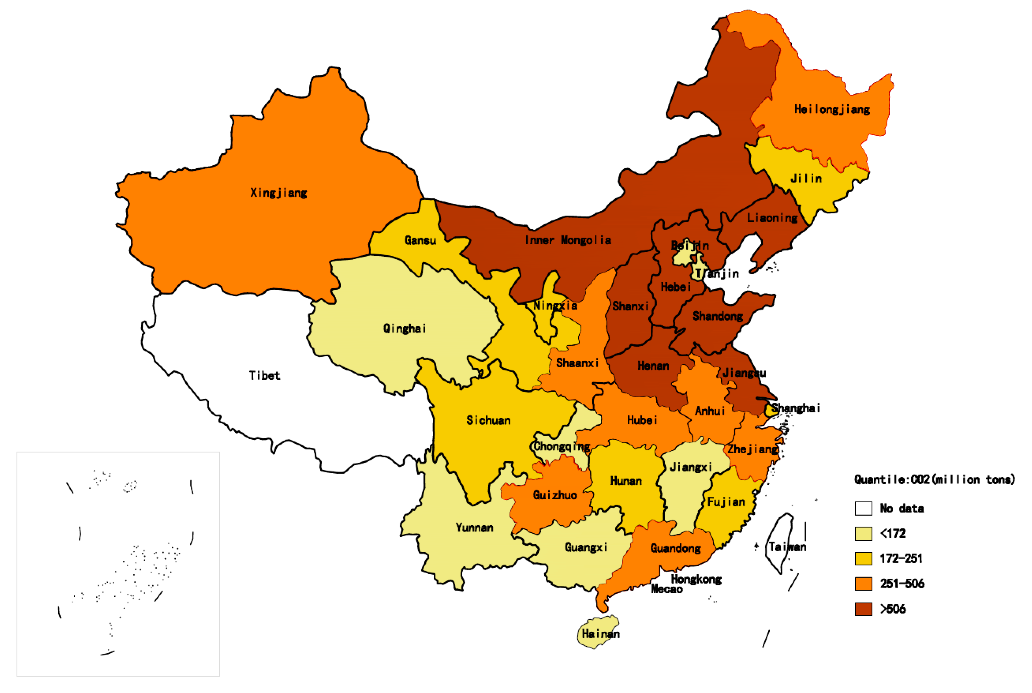
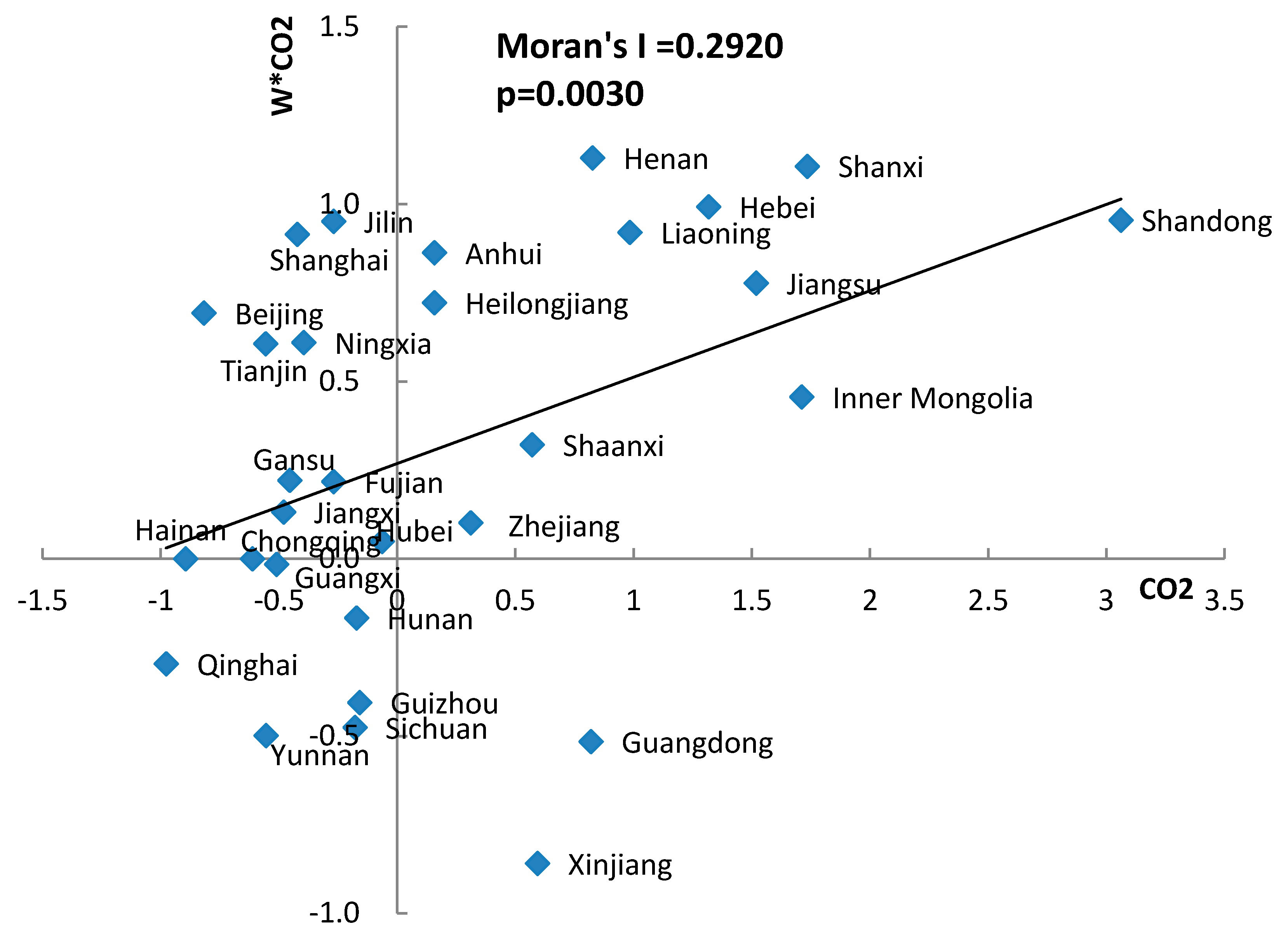
4.1.2. Test for Spatial Dependence of Provincial Carbon Emissions

According to Equation (9), we calculate Moran’s I to test for the existence of spatial dependence of provincial carbon emissions in China between 1998–2015. The results are provided in

Table 3. Moran’s I of regional carbon emissions from 1998–2015.

Year	Moran’s I	Z	p Value
1998	0.2550	2.6060	0.0090
1999	0.2980	2.9710	0.0030
2000	0.2710	2.7410	0.0060
2001	0.3140	3.1170	0.0020
2002	0.3120	3.1120	0.0020
2003	0.2820	2.8520	0.0040
2004	0.3240	3.2120	0.0010
2005	0.3610	3.5720	0.0000
2006	0.3440	3.4420	0.0010
2007	0.3500	3.4800	0.0010
2008	0.3510	3.5220	0.0000
2009	0.3270	3.2990	0.0010
2010	0.3230	3.2590	0.0010
2011	0.3270	3.2510	0.0010
2012	0.3130	3.1450	0.0020
2013	0.3320	3.3010	0.0010
2014	0.3090	3.1230	0.0020
2015	0.2920	2.9860	0.0030

Data source: The Moran’s I statistics are calculated by carbon emissions based on energy consumption data from the China Statistical Yearbook.

, which shows that Moran’s I is significantly positive every year. This implies carbon emissions in the 30 Chinese provinces have a positive spatial correlation on average.

Given that Moran’s I only reveals the overall trend of spatial correlation, and cannot identify any idiosyncratic individual observations, Moran scatter plot is used to illustrate the relationship between each observation with its neighbors. Figure 1 shows Moran scatter for provincial carbon emissions in 2015. The provinces in Quadrants I and III both indicate a positive spatial correlation or a spatial cluster of similar carbon emissions. 11 high-emission provinces (36.7%) in Quadrant I with high-emission neighbors are those consume more coal in terms of both amount and proportion, such as Shanxi, Inner Mongolia, and Shandong. According to the National Bureau of Statistics of China, each of these three provinces consumed more than 360 million tons of coal every year, making up more than 70 percent of their total consumed energy in recent years. 7 provinces (23.3%) in Quadrant III represent low-emission provinces, mostly in the southwest (such as Sichuan, Yunnan, Guizhou, Qinghai, and Guangxi), with low-emission neighbors.

The remaining points in Quadrants II and IV represent low- and high-emission provinces surrounded by high- and low-emission provinces respectively. They both stand for negative spatial correlations [55]. 12 provinces (40%) are in Quadrants II and IV, with provinces that include Beijing, Shanghai, and Tianjin being low-emission areas with high-emissions in neighboring provinces; Guangdong and Xinjiang are high-emission provinces with low-emission neighbors.

Figure 2 depicts the spatial distribution map of the 30 provinces’ 2015 carbon emissions. Consistent with findings of Figure 1, there are obvious spatial clusters. Moreover, most provinces with high and low carbon emissions are located in the north and southwest respectively.

Moran’s I and the Moran scatter plot show that provinces’ carbon emissions are significantly correlated and therefore appropriate spatial models need to be established. First, it is necessary to test for the presence of spatial effects. To do this, we conduct the Lagrange Multiplier (LM) tests for a spatially lagged dependent variable (LM spatial lag) and a spatial auto-correlated error term (LM spatial error) through the OLS regression of Equations (3) and (4), i.e., Models 1 and 2. If the results of LM tests reject the hypothesis of no-spatial lag or error effect, we need further estimate the SDM to conduct Wald tests and LR tests. The hypotheses of Wald include $H_0:\theta =0$ and $H_0:\theta +\rho \beta =0$, the former testing for whether the SDM can be simplified to the SLM and the latter for whether the SDM can be simplified to the SEM [46]. These can also be done by LR tests.

Table 4. Diagnostic test results of spatial specification.

	Model 1 (OLS)	Model 2 (OLS)	Model 3 (SDM)	Model 4 (SDM)
LM spatial lag	1.4001 (0.2370)	1.9685 (0.1610)
Robust LM spatial lag	6.2375 (0.0130)	16.6173 (0.0000)
LM spatial error	3.4277 (0.0640)	1.1560 (0.2820)
Robust LM spatial error	8.2651 (0.0040)	15.8048 (0.0000)
Wald spatial lag			171.6849 (0.0000)	198.0819 (0.0000)
LR spatial lag			145.9280 (0.0000)	162.7944 (0.0000)
Wald spatial error			156.8946 (0.0000)	185.5712 (0.0000)
LR spatial error			142.6244 (0.0000)	162.5676 (0.0000)

Note: The p-values of corresponding statistics are reported in parentheses. Data source: The statistics are from the regression results of Models 1–4.

contains the results of these tests, indicating that the robust LM spatial lag rejects the null hypothesis of no-spatial lag effect in Model 1 and Model 2, and robust LM spatial error reject the null hypothesis of no-spatial error effect in Model 1 and Model 2. Then we estimate the SDMs, i.e., Models 3 and 4, according to Equations (5) and (6), with the Wald and LR test results in Table 4 strongly rejecting the null hypotheses of simplifying the SDM to either the SLM or SEM. Therefore, the SDM is the most appropriate model specification for our estimation.

4.2. Regression Results with Spatial Effects

Table 5. Results of Models 1–4.

Regressor	Model 1	Model 3	Regressor	Model 2	Model 4
$\ln PGDP$	0.9247 ***	1.0822 ***	$\ln PGDP$	0.6951 ***	1.1073 ***
$\ln pop$	1.3383 ***	0.8743 ***
$\ln RD$	0.5643 ***	0.2061 *	$\ln PRD$	0.4289 ***	0.1564 ***
$\ln patent$	−0.0460 *	−0.0502 *	$\ln patent$	−0.0587 **	−0.0487
$\ln FDI$	−0.0347 **	−0.0481 ***	$\ln PFDI$	−0.0494 ***	−0.0684 ***
$\ln service$	−0.3228 ***	0.3195 ***	$\ln instr$	−0.0968	0.3470 ***
$\ln coalc$	0.8714 ***	1.1683 ***	$\ln enstr$	0.7831 ***	1.1426 ***
$\ln PGDP*\ln RD$	−0.0466 ***	−0.0222 **	$\ln PGDP*\ln PRD$	−0.0299 ***	-0.0165 ***
$W*\ln CO2$		0.2260 ***	$W*\ln PCO2$		0.2490 ***
$W*\ln PGDP$		0.1863	$W*\ln PGDP$		0.5341 ***
$W*\ln pop$		0.2438 **
$W*\ln RD$		−1.2138 ***	$W*\ln PRD$		−0.2974 ***
$W*\ln patent$		−0.0984 **	$W*\ln patent$		−0.1394 ***
$W*\ln FDI$		−0.2520 ***	$W*\ln PFDI$		−0.2763 ***
$W*\ln service$		−0.8829 ***	$W*\ln instr$		−0.4334 *
$W*\ln coalc$		−0.2221 **	$W*\ln enstr$		−0.2692 **
$W*\ln PGDP*\ln RD$		0.1131 ***	$W*\ln PGDP*\ln PRD$		0.0236 ***
Observations	540	540	Observations	540	540
Corrected R2	0.9021	0.9057	Corrected R2	0.5450	0.8230
log-likelihood		10.3169	log-likelihood		4.9750
integration order	I(0)	I(0)		I(0)	I(0)
Pesaran CD test	−1.86 *	−2.34		−1.95 *	−1.01

Note: ***, ** and * indicate significance at 1%, 5% and 10% level respectively. Data source: The coefficients and statistics are from the regression results of Models 1–4. Order of integration of the residuals is determined from the Pesaran (2007) CIPS test: I(0) = stationary.

provides the regression results of Models 1–2, and the point estimates of Models 3–4. According to Equation (8), by the partial derivative of the dependent variable with respect to the explanatory variables, we acquire the direct effects and more accurate spatial spillover effects from Models 3–4 (

Table 6. Direct and spatial spillover effects of Models 3 and 4.

Model 3	Direct Effects	Spatial Spillover Effects	Model 4	Direct Effects	Spatial Spillover Effects
$\ln PGDP$	1.1053 ***	0.5242 ***	$\ln PGDP$	1.1567 ***	1.0291 ***
$\ln pop$	0.8999 ***	0.5390 ***
$\ln RD$	0.1328	−1.4315 ***	$\ln PRD$	0.1415 ***	−0.3286 ***
$\ln patent$	−0.0564 *	−0.1341 **	$\ln patent$	−0.0590 *	−0.1934 ***
$\ln FDI$	−0.0633 ***	−0.3223 ***	$\ln PFDI$	−0.0869 ***	−0.3713 ***
$\ln service$	0.2729 **	−0.9926 ***	$\ln instr$	0.3221 ***	−0.4521
$\ln coalc$	1.1698 ***	0.0581	$\ln enstr$	1.1442 ***	0.0190
$\ln PGDP*\ln RD$	−0.0154 *	0.1326 ***	$\ln PGDP*\ln PRPD$	−0.0153 ***	0.0248 **

Note: ***, ** and * indicate significance at the 1%, 5% and 10% level, respectively. Data source: The coefficients and statistics are from the regression results of Models 3–4.

). The direct effects denote the impact of the explanatory variables in a particular region on local carbon emissions, while the spatial spillover effects denote the impact of the explanatory variables in a particular region on the carbon emissions of its neighbors. The spatial autoregressive coefficient ($W*\ln CO2$) is significantly positive in both Modes 3 and 4. The positive coefficients indicate that, on average, carbon emissions (per capita) in a particular province are positively influenced by its neighboring provinces. This result is consistent with Kang et al. [56], who find that the carbon emissions in neighboring regions have a positive effect on local carbon emissions in China.

In addition, we further test whether the residuals are cross-section independence by the Pesaran CD test [57]. As shown in Table 5, the Pesaran CD test results of residuals of Models 1–4 cannot reject the null hypothesis of cross-section independence at the 5% significance level. Thus, the residuals of Model 3 and Model 4 are cross-sectionally uncorrelated statistically. To show the stationary of the residuals of Models 1–4, we also do the Pesaran (2007) panel unit root test of the residuals of Models 1–4. The results for both residuals of Models 1–4 reject the null hypothesis of unit root, thus showing that the residuals are stationary.

4.2.1. Direct Moderating Effects of R&D Investment

In terms of the direct effect of R&D investment on the relationship of income and carbon emissions, we combine Table 5 and Table 6 to find that: R&D investment directly moderates the positive effect of income on carbon emissions in local provinces, and more R&D investment can enforce an earlier turning point for local carbon emissions. Specifically, from the direct effects results of Model 3 in Table 6, the interaction of income and R&D investment contributes to decreasing carbon emissions because of the significantly negative coefficient −0.0154, and income has positive impact on carbon emissions because of the significantly positive coefficient 1.1053. The results indicate that, when the logarithmic GDP per capita is less than $1.1053/(0.0154*\ln RD)$, carbon emissions increase with increasing income; when the logarithmic GDP per capita is more than $1.1053/(0.0154*\ln RD)$, carbon emissions decrease with increasing income; and when the logarithmic GDP per capita is equal to $1.1053/(0.0154*\ln RD)$, carbon emissions reach the turning point with other conditions unchanged. In addition, in Model 1 without the spatial effect, the significantly negative coefficient of the interaction of income and R&D investment, as well as the significantly positive coefficient of income also indicate that, R&D investment moderates the effect that economic development increases carbon emissions: when the logarithmic GDP per capita is equal to $0.9247/(0.0466*\ln RD)$, carbon emissions reach the turning point with other conditions unchanged; when the logarithmic GDP per capita is more than $0.9247/(0.0466*\ln RD)$, carbon emissions decrease with increasing income.

The significantly positive direct effect of $\ln PGDP$ and the significantly negative direct effect of $\ln PGDP*\ln PRD$ in Model 4 in Table 6 indicate that, when the logarithmic GDP per capita is less than $1.1567/(0.0153*\ln PRD)$, carbon emissions per capita increase with increasing income; when the logarithmic GDP per capita is more than $1.1567/(0.0153*\ln PRD)$, carbon emissions per capita decrease with increasing income; and when the logarithmic GDP per capita is equal to $1.1567/(0.0153*\ln PRD)$, carbon emissions per capita reach the turning point with other conditions unchanged. The results of Model 2 without the spatial effect also signify that more R&D investment per capita can constrain the increase of carbon emissions per capita, with carbon emissions per capita reaching the turning point when the logarithmic GDP per capita is $0.6951/(0.0299*\ln PRD)$.

From the results of traditional model and spatial model, we can draw a conclusion that income contributes to the carbon emissions increase, but the impact is restrained by R&D investment, and R&D investment moderates the impact even to the opposite direction. R&D investment is transformed into technological achievements, and promotes technological progress. The application of advanced technology is beneficial for cleanly and efficiently exploiting and utilizing energy, and improving production efficiency, which constrains the process of China releasing increased carbon emissions as economic development occurs. For the sake of saving energy and reducing carbon emissions, on the one hand, Chinese government is accelerating the R&D investment of energy saving and carbon emissions reduction technology; on the other hand, regulatory policies such as energy efficiency improvement and carbon emissions trading indirectly prompt enterprises to invest in low-carbon technologies. Therefore, with increasing incomes, R&D investment constrains the positive impact of income on carbon emissions. The moderating effects of R&D investment reflect that technological progress plays a vital role in the process of low carbon economic development.

4.2.2. Spatial Spillover Moderating Effect of R&D Investment

As for the spatial spillover moderating effect of R&D investment on the relationship of income and carbon emissions, we find that R&D investment in local provinces increases the positive influence of local income on neighboring carbon emissions. As is shown in Model 3 in Table 6, the spatial spillover effect of the interaction term coefficient ($W*\ln PGDP*\ln RD$) is significantly positive, which indicates that the greater the local R&D investment, the stronger the influence of local income on neighboring carbon emissions. It should be noted that the spillover effects of income on neighboring carbon emissions ($W*\ln PGDP$) are significantly positive in Model 3. Such a spillover effect of income on carbon emissions is expected to be positive, because income improvement in a region is inclined towards increasing incomes in the neighboring regions, which increases neighboring carbon emissions. From the results of Model 4 in Table 6, the spatial spillover moderating effect of interaction term coefficient ($W*\ln PGDP*\ln PRD$) is significantly positive, and the spatial spillover effect of income ($W*\ln PGDP$) on carbon emissions per capita is significantly positive, which also supports that R&D investment per capita increases the positive effect of local income on neighboring carbon emissions per capita.

Generally, more R&D investment increases the positive spatial spillover effect of local income on neighboring carbon emissions. This result indicates that the transfer effect of carbon emissions plays the dominate role rather than the knowledge spillover effect among the neighboring regions. Generally, regions with higher R&D investment have a relatively high level of economic development and environmental regulations. Rich regions with strict environmental regulations will transfer backward industries to the less regulated neighboring regions with relatively low levels in terms of economic development [58], which promotes the carbon emissions increase in the neighboring regions. Furthermore, a relatively high technology level in a province decreases the competitiveness of enterprises with lower technology, and this type of enterprises may be built or operated in neighboring provinces with a lower competitiveness. Hence, carbon emissions experience an increase in these neighboring provinces with lagging technology or production efficiency. If the spatial effect is not considered, then the spillover moderating effect of R&D on income-CO2 will be neglected.

4.2.3. Direct and Spatial Spillover Effects of Other Influencing Factors

According to Table 6, the direct and spillover effects of other influencing factors are:

(1)

Coal consumption is the main driving force in increasing local carbon emissions, while the spatial spillover effect of energy structure on neighboring carbon emissions is insignificant. Specifically, the direct effects in Table 6 show a 1% decrease in the coal consumption/total energy consumption leads to an approximate 1.17% (1.14%) decrease in local carbon emissions (per capita), with other conditions unchanged. These results are similar to those of Zhang et al. [59] who also find coal consumption has a major positive effect on carbon emissions. This is because China’s energy supply mainly depends on coal, and coal consumption is the main source of energy-related carbon emissions in China. However, the spatial spillover effects of energy structure in Models 3–4 are not significant.

(2)

FDI contributes to constraining both local and neighboring carbon emissions. Specifically, the direct effects of FDI are significantly negative (approximately −0.06 and −0.09) in Model 3 and Model 4, respectively, and the spatial spillover effects are both significantly negative in Models 3 and 4. FDI reduces carbon emissions by introducing advanced technologies of energy conservation, and promoting the technological progress of enterprises. As is explained by Wang et al. [60], if each region can introduce more advanced technologies and more investment from environmental enterprises, FDI can have a positive effect on upgrading the environment performance. This result is also supported by Zhou et al. [61], who found that FDI reduces carbon emissions when analyzing the relationship between industrial structural transformation and carbon dioxide emissions in China.

(3)

Patents have an impact on constraining both local and neighboring carbon emissions. The direct effect of patents is significantly negative in both Model 3 and Model 4 at approximately −0.06. The spillover effects of patents are significantly negative in both Model 3 and Model 4, indicating that a province’s patents increase can constrain carbon emissions (per capita) in its neighboring provinces. The application of technological output can improve energy efficiency to some extent and has a negative impact on carbon emissions.

4.3. Robust Analysis for the Moderating Effect of R&D Investment

To ensure whether the empirical results of the direct and spatial moderating role of R&D investment are robust, we further do the robust analysis of Models 3–4 in the three cases: (1) Use the economic distance as the spatial weight matrix rather than the geographical distance, i.e.,$w_{ij}=1/\left|\overline{y_i}-\overline{y_j}\right|$, where $\overline{y_i}$ and $\overline{y_j}$ are the average regional income during the same period of provinces $i$ and $j$. (2) Include the coal deposits (represented by coal production of 30 provinces during the sample period) as the explanatory variable, given that carbon emissions may be spatially clustered because the coal deposits are spatially clustered. (3) Replace the contemporaneous R&D (R&D per capita) and FDI (FDI per capita) with the lag one, as R&D and FDI may have a lagged effect on carbon emissions. The regression results of the three cases of Model 3 and Model 4 are shown in columns (1) (2) (3) of

Table 7. Robust analysis of Model 3.

Regressor	(1)	(2)	(3)
$\ln PGDP$	0.8705 ***	1.0835 ***	1.0623 ***
$\ln pop$	1.1282 ***	0.8776 ***	0.9214 ***
$\ln RD$	0.7068 ***	0.2106 *	0.0366
$\ln patent$	−0.0138	−0.0516 *	−0.0620 **
$\ln FDI$	−0.0420 ***	−0.0479 ***	−0.0516 ***
$\ln service$	−0.0012	0.3248 ***	0.3376 ***
$\ln coalc$	0.7882 ***	1.1694 ***	1.1494 ***
$\ln coalp$		−0.0014
$\ln PGDP*\ln RD$	−0.0628 ***	−0.0227 *	−0.0057
$W*\ln CO2$	0.1710 ***	0.2300 ***	0.1090 **
$W*\ln PGDP$	0.1853	0.1749	0.2220 ***
$W*\ln pop$	0.3057	0.2352 **	0.3636 **
$W*\ln RD$	−0.4141 ***	−1.2254 ***	0.1968 *
$W*\ln patent$	−0.0499	−0.0950 *	−0.5056 ***
$W*\ln FDI$	0.0038	−0.2512 ***	−0.1039 **
$W*\ln service$	−0.7524 ***	−0.9006 ***	−0.6151 ***
$W*\ln coalc$	0.0964	−0.2259 *	−0.2295 **
$W*\ln coalp$		0.0014
$W*\ln PGDP*\ln RD$	0.0460 ***	0.1143 ***	0.0498 ***
Observations	540	540	540
Corrected R2	0.9112	0.9056	0.8352
log-likelihood	295.1855	10.1476	282.5486

Note: ***, ** and * indicate significance at 1%, 5% and 10% level respectively. Data source: The coefficients and statistics are from the regression results of robust analysis in terms of Model 3.

and

Table 8. Robust analysis of Model 4.

Regressor	(1)	(2)	(3)
$\ln PGDP$	0.7426 ***	1.1186 ***	1.1347 ***
$\ln PRD$	0.5020 ***	0.1278 ***	0.1164 ***
$\ln patent$	−0.0422 *	−0.0617 **	−0.0657 **
$\ln PFDI$	−0.0498 ***	−0.0618 ***	−0.0668 ***
$\ln service$	−0.0336	0.3305 ***	0.3707 ***
$\ln coalc$	0.7162 ***	1.1621 ***	1.1345 ***
$\ln coalp$		-0.0020
$\ln PGDP*\ln PRD$	−0.0403 ***	−0.0141 ***	-0.0133 ***
$W*\ln PCO2$	0.1870 ***	0.2630 ***	0.2330 ***
$W*\ln PGDP$	0.0951	0.5417 ***	0.5936 ***
$W*\ln PRD$	−0.4310 ***	−0.2777 ***	−0.2752 ***
$W*\ln patent$	−0.0505	−0.1504 ***	−0.1417 ***
$W*\ln PFDI$	−0.0018	−0.2972 ***	−0.2990 ***
$W*\ln service$	−0.7101 ***	−0.4679 **	−0.4060 **
$W*\ln coalc$	0.0380	−0.2685 **	−0.2857 **
$W*\ln coalp$		−0.0151
$W*\ln PGDP*\ln PRD$	0.0487 ***	0.0233 ***	0.0227 ***
Observations	540	540	540
Corrected R2	0.8948	0.8249	0.8852
log-likelihood	284.8129	8.3711	7.3087

Note: ***, ** and * indicate significance at 1%, 5% and 10% level respectively. Data source: The coefficients and statistics are from the regression results of robust analysis in terms of Model 4.

, respectively.

For the direct moderating effect of R&D investment on income-carbon emissions, we can find that income promotes local carbon emissions due to the significantly positive coefficients of $\ln PGDP$ in both Table 7 and Table 8, whereas the coefficients of $\ln PGDP*\ln RD$ in the three cases in Table 7 and Table 8 are negative, with column (1) in Table 7 and all in Table 8 being significant at the 1% level. The results indicate that income promotes carbon emissions increases, but the impact can be constrained by the R&D investment, which is generally consistent with the findings of Model 3 and Model 4. As for the spatial moderating effect of R&D investment on income-carbon emissions, we can find that the coefficients of $W*\ln PGDP$ in the three cases in Table 7 and Table 8 are positive, with column (3) in Table 7 and columns (2) (3) in Table 8 being significantly positive at the 1% level, moreover, the coefficients of $W*\ln PGDP*\ln RD$ are significantly positive at the 1% level in all the cases. The results disclose that R&D investment promotes the effect that local income increases neighboring regions’ carbon emissions, which confirms the findings of Model 3 and Model 4. Thus, we can conclude that the direct moderating effect of R&D investment can constrain the carbon emissions as income increases, whereas the spatial moderating effect of R&D investment promotes the neighboring carbon emissions increase. In addition, the findings that coal consumption is the main driving force in increasing local carbon emissions, and FDI and patents are the main constrained forces in increasing both local and neighboring carbon emissions are also supported.

5. Conclusions and Policy Implications

This paper develops a spatial Durbin model (SDM) to analyze the direct and spatial spillover moderating effects of R&D investment on the relationship between income and carbon emissions, and the direct and spillover effects of energy structure, FDI, and patents on carbon emissions by controlling the spatial dependence. This is applied to the data of 30 Chinese provinces during 1998–2015. The main findings are that:

(1)

R&D investment constrains the positive effects of income on local carbon emissions. The corresponding income level of the turning point in local carbon emissions depends on R&D investment, and more R&D investment results in carbon emissions reaching a turning point earlier. Income contributes to the increase in local carbon emissions, but the impact is restrained by R&D investment, with R&D investment moderating the impact even to the opposite direction.

(2)

R&D investment in local provinces generally increases the positive influence of local income on neighboring carbon emissions, because the carbon emissions transfer effect driven by R&D investment plays the dominate role rather than the knowledge spillover effect.

(3)

The proportion of coal consumption to total energy consumption is the main driver of local carbon emissions. FDI and patents generally constrain carbon emissions not only in local provinces but also in neighboring provinces.

These results have policy implications, in that R&D investment can be enhanced in provinces where their economy develops at the cost of environmental quality, so that their carbon emissions reach a turning point earlier with the increase of income because of the moderating effect of R&D investment on low carbon economic development. In addition, provinces with lower income should not relax their environmental regulations in the case of alleviating the carbon emissions transfer effect; they should learn or absorb the technological innovation from the neighboring provinces to increase the knowledge spillovers effect. Policy makers can also reduce the appropriate proportion of coal consumption, and increase FDI and patents to reduce carbon emissions in both local and neighboring provinces.

Many opportunities exist for future work. For instance, further research could analyze the impact of some indicators on environmental pollution by considering the spatial weight matrix of economic relations rather than geographical locations. Other research can also be carried out to investigate the effects of energy-related technological progress or green technologies on environmental pollution.

References

1. Zhang, Y.J.; Liu, Z.; Zhang, H.; Tan, T.D. The impact of economic growth, industrial structure and urbanization on carbon emission intensity in China. Nat. Hazards 2014, 73, 579–595. [Google Scholar] [CrossRef]
2. Ma, C.; Stern, D.I. China’s changing energy intensity trend: A decomposition analysis. Energy Econ. 2008, 30, 1037–1053. [Google Scholar] [CrossRef]
3. Liu, Q.; Wang, Q. Sources and flows of China’s virtual SO2 emission transfers embodied in interprovincial trade: A multiregional input–output analysis. J. Clean. Prod. 2017, 161, 735–747. [Google Scholar] [CrossRef]
4. Jiao, J.; Jiang, G.; Yang, R. Impact of R&D technology spillovers on carbon emissions between China’s regions. Struct. Chang. Econ. Dyn. 2018, 47, 35–45. [Google Scholar]
5. Huang, J.; Du, D.; Tao, Q. An analysis of technological factors and energy intensity in China. Energy Policy 2017, 109, 1–9. [Google Scholar] [CrossRef]
6. Huang, J.; Hao, Y.; Lei, H. Indigenous versus foreign innovation and energy intensity in China. Renew. Sustain. Energy Rev. 2018, 81, 1721–1729. [Google Scholar] [CrossRef]
7. Ghisetti, C.; Pontoni, F. Investigating policy and R&D effects on environmental innovation: A meta-analysis. Ecol. Econ. 2015, 118, 57–66. [Google Scholar]
8. Kaya, Y. Impact of Carbon Dioxide Emission Control on GNP Growth: Interpretation of Proposed Scenarios; Intergovernmental Panel on Climate Change/Response Strategies Working Group: Pairs, France, May 1989.
9. Ehrlich, P.R.; Holdren, J.P. Impact of population growth. Science 1971, 171, 1212–1217. [Google Scholar] [CrossRef] [PubMed]
10. Yin, J.; Zheng, M.; Chen, J. The effects of environmental regulation and technical progress on CO2 Kuznets curve: An evidence from China. Energy Policy 2015, 77, 97–108. [Google Scholar] [CrossRef]
11. Stern, D.I. The rise and fall of the environmental Kuznets curve. World Dev. 2004, 32, 1419–1439. [Google Scholar] [CrossRef]
12. Narayan, P.K.; Narayan, S. Carbon dioxide emissions and economic growth: Panel data evidence from developing countries. Energy Policy 2010, 38, 661–666. [Google Scholar] [CrossRef]
13. Agras, J.; Chapman, D. A dynamic approach to the Environmental Kuznets Curve hypothesis. Ecol. Econ. 1999, 28, 267–277. [Google Scholar] [CrossRef]
14. Cheng, Z.; Li, L.; Liu, J. Industrial structure, technical progress and carbon intensity in China’s provinces. Renew. Sustain. Energy Rev. 2018, 81, 2935–2946. [Google Scholar] [CrossRef]
15. Fan, Y.; Liu, L.C.; Wu, G.; Wei, Y.M. Analyzing impact factors of CO2 emissions using the STIRPAT model. Environ. Impact Assess. Rev. 2006, 26, 377–395. [Google Scholar] [CrossRef]
16. Liu, Y.; Zhou, Y.; Wu, W. Assessing the impact of population, income and technology on energy consumption and industrial pollutant emissions in China. Appl. Energy 2015, 155, 904–917. [Google Scholar] [CrossRef]
17. Albino, V.; Ardito, L.; Dangelico, R.M.; Petruzzelli, A.M. Understanding the development trends of low-carbon energy technologies: A patent analysis. Appl. Energy 2014, 135, 836–854. [Google Scholar] [CrossRef]
18. Al-Mulali, U.; Sheau-Ting, L. Econometric analysis of trade, exports, imports, energy consumption and CO2 emission in six regions. Renew. Sustain. Energy Rev. 2014, 33, 484–498. [Google Scholar] [CrossRef]
19. Lee, J.W. The contribution of foreign direct investment to clean energy use, carbon emissions and economic growth. Energy Policy 2013, 55, 483–489. [Google Scholar] [CrossRef]
20. Huang, J.; Liu, Q.; Cai, X.; Hao, Y.; Lei, H. The effect of technological factors on China’s carbon intensity: New evidence from a panel threshold model. Energy Policy 2018, 115, 32–42. [Google Scholar] [CrossRef]
21. Yang, Y.; Cai, W.; Wang, C. Industrial CO2 intensity, indigenous innovation and R&D spillovers in China’s provinces. Appl. Energy 2014, 131, 117–127. [Google Scholar]
22. Kaika, D.; Zervas, E. The environmental Kuznets curve (EKC) theory. Part B: Critical issues. Energy Policy 2013, 62, 1403–1411. [Google Scholar] [CrossRef]
23. Cheng, Z.; Li, L.; Liu, J. The emissions reduction effect and technical progress effect of environmental regulation policy tools. J. Clean. Prod. 2017, 149, 191–205. [Google Scholar] [CrossRef]
24. Hao, Y.; Liu, Y.M. The influential factors of urban PM2.5 concentrations in China: A spatial econometric analysis. J. Clean. Prod. 2016, 112, 1443–1453. [Google Scholar] [CrossRef]
25. Burnett, J.W.; Bergstrom, J.C.; Dorfman, J.H. A spatial panel data approach to estimating US state-level energy emissions. Energy Econ. 2013, 40, 396–404. [Google Scholar] [CrossRef]
26. Cheng, Z.; Li, L.; Liu, J. Identifying the spatial effects and driving factors of urban PM2.5 pollution in China. Ecol. Indic. 2017, 82, 61–75. [Google Scholar] [CrossRef]
27. Hao, Y.; Liu, Y.; Weng, J.H.; Gao, Y. Does the Environmental Kuznets Curve for coal consumption in China exist? New evidence from spatial econometric analysis. Energy 2016, 114, 1214–1223. [Google Scholar] [CrossRef]
28. Li, L.; Hong, X.; Peng, K. A spatial panel analysis of carbon emissions, economic growth and high-technology industry in China. Struct. Chang. Econ. Dyn. 2018. [Google Scholar] [CrossRef]
29. Yang, Y.; Zhou, Y.; Poon, J.; He, Z. China’s carbon dioxide emission and driving factors: A spatial analysis. J. Clean. Prod. 2019, 211, 640–651. [Google Scholar] [CrossRef]
30. Guo, J.; Zhang, Z.; Meng, L. China’s provincial CO2 emissions embodied in international and interprovincial trade. Energy Policy 2012, 42, 486–497. [Google Scholar] [CrossRef]
31. Zhang, Z.; Guo, J.; Hewings, G.J.D. The effects of direct trade within China on regional and national CO2 emissions. Energy Econ. 2014, 46, 161–175. [Google Scholar] [CrossRef]
32. Wu, A.; Li, G.; Sun, T.; Liang, Y. Effects of industrial relocation on Chinese regional economic growth disparities: Based on system dynamics modeling. Chin. Geogr. Sci. 2014, 24, 706–716. [Google Scholar] [CrossRef]
33. Xu, J.; Zhang, M.; Zhou, M.; Li, H. An empirical study on the dynamic effect of regional industrial carbon transfer in China. Ecol. Indic. 2017, 73, 1–10. [Google Scholar] [CrossRef]
34. Sun, L.; Wang, Q.; Zhou, P.; Cheng, F. Effects of carbon emission transfer on economic spillover and carbon emission reduction in China. J. Clean. Prod. 2016, 112, 1432–1442. [Google Scholar] [CrossRef]
35. Liobikienė, G.; Butkus, M. Environmental Kuznets Curve of greenhouse gas emissions including technological progress and substitution effects. Energy 2017, 135, 237–248. [Google Scholar] [CrossRef]
36. Dietz, T.; Rosa, E.A. Effects of population and affluence on CO2 emissions. Proc. Natl. Acad. Sci. USA 1997, 94, 175–179. [Google Scholar] [CrossRef] [PubMed]
37. Shao, S.; Yang, L.; Yu, M.; Yu, M. Estimation, characteristics, and determinants of energy-related industrial CO2 emissions in Shanghai (China), 1994–2009. Energy Policy 2011, 39, 6476–6494. [Google Scholar] [CrossRef]
38. York, R.; Rosa, E.A.; Dietz, T. STIRPAT, IPAT and ImPACT: Analytic tools for unpacking the driving forces of environmental impacts. Ecol. Econ. 2003, 46, 351–365. [Google Scholar] [CrossRef]
39. Iwata, H.; Okada, K.; Samreth, S. A note on the environmental Kuznets curve for CO2: A pooled mean group approach. Appl. Energy 2011, 88, 1986–1996. [Google Scholar] [CrossRef]
40. Yuan, J.; Xu, Y.; Hu, Z.; Zhao, C.; Xiong, M.; Guo, J. Peak energy consumption and CO2 emissions in China. Energy Policy 2014, 68, 508–523. [Google Scholar] [CrossRef]
41. He, J.; Wang, H. Economic structure, development policy and environmental quality: An empirical analysis of environmental Kuznets curves with Chinese municipal data. Ecol. Econ. 2012, 76, 49–59. [Google Scholar] [CrossRef]
42. Wang, P.; Wu, W.; Zhu, B.; Wei, Y. Examining the impact factors of energy-related CO2 emissions using the STIRPAT model in Guangdong Province, China. Appl. Energy 2013, 106, 65–71. [Google Scholar] [CrossRef]
43. Zhao, C.; Chen, B.; Hayat, T.; Alsaedi, A.; Ahmad, B. Driving force analysis of water footprint change based on extended STIRPAT model: Evidence from the Chinese agricultural sector. Ecol. Indic. 2014, 47, 43–49. [Google Scholar] [CrossRef]
44. Ren, S.; Yuan, B.; Ma, X.; Chen, X. The impact of international trade on China’s industrial carbon emissions since its entry into WTO. Energy Policy 2014, 69, 624–634. [Google Scholar] [CrossRef]
45. Wang, C.; Wang, F.; Zhang, X.; Yang, Y.; Su, Y.; Ye, Y.; Zhang, H. Examining the driving factors of energy related carbon emissions using the extended STIRPAT model based on IPAT identity in Xinjiang. Renew. Sustain. Energy Rev. 2017, 67, 51–61. [Google Scholar] [CrossRef]
46. Burridge, P. Testing for a common factor in a spatial autoregression model. Environ. Plan. A 1981, 13, 795–800. [Google Scholar] [CrossRef]
47. Lesage, J.; Pace, R.K. Introduction to Spatial Econometrics; CRC Press: New York, NY, USA, 2009; Available online: https://journals.openedition.org/rei/pdf/3887.
48. Elhorst, J.P. Spatial Econometrics: From Cross-Sectional Data to Spatial Panels; Springer: Berlin, Germany, 2014. [Google Scholar]
49. Huang, Y. Drivers of rising global energy demand: The importance of spatial lag and error dependence. Energy 2014, 76, 254–263. [Google Scholar] [CrossRef]
50. Zhang, Y.J.; Hao, J.F.; Song, J. The CO2 emission efficiency, reduction potential and spatial clustering in China’s industry: Evidence from the regional level. Appl. Energy 2016, 174, 213–223. [Google Scholar] [CrossRef]
51. Eggleston, H.S.; Buendia, L.; Miwa, K.; Ngara, T.; Tanabe, K. IPCC Guidelines for National Greenhouse Gas Inventories; Institute for Global Environmental Strategies: Hayama, Japan, 2006; Volume 2, pp. 48–56. [Google Scholar]
52. Zhang, Y.J.; Da, Y.B. The decomposition of energy-related carbon emission and its decoupling with economic growth in China. Renew. Sustain. Energy Rev. 2015, 41, 1255–1266. [Google Scholar] [CrossRef]
53. Pesaran, M.H. A simple panel unit root test in the presence of cross-section dependence. J. Appl. Econom. 2007, 22, 265–312. [Google Scholar] [CrossRef]
54. Liddle, B.; Lung, S. Revisiting energy consumption and GDP causality: Importance of a priori hypothesis testing, disaggregated data, and heterogeneous panels. Appl. Energy 2015, 142, 44–55. [Google Scholar] [CrossRef]
55. Huang, Q.; Chand, S. Spatial spillovers of regional wages: Evidence from Chinese provinces. China Econ. Rev. 2015, 32, 97–109. [Google Scholar] [CrossRef]
56. Kang, Y.Q.; Zhao, T.; Yang, Y.Y. Environmental Kuznets curve for CO2 emissions in China: A spatial panel data approach. Ecol. Indic. 2016, 63, 231–239. [Google Scholar] [CrossRef]
57. Pesaran, M.H. General Diagnostic Tests for Cross Section Dependence in Panels; Cambridge Working Papers in Economics; Institute for the Study of Labor (IZA): Bonn, Germany, 2004; Volume 69, p. 1240. [Google Scholar]
58. Liu, L.C.; Fan, Y.; Wu, G.; Wei, Y.M. Using LMDI method to analyze the change of China’s industrial CO2 emissions from final fuel use: An empirical analysis. Energy Policy 2007, 35, 5892–5900. [Google Scholar] [CrossRef]
59. Zhang, Q.; Yang, J.; Sun, Z.; Wu, F. Analyzing the impact factors of energy-related CO2 emissions in China: What can spatial panel regressions tell us? J. Clean. Prod. 2017, 161, 1085–1093. [Google Scholar] [CrossRef]
60. Wang, Z.; Zhang, B.; Liu, T. Empirical analysis on the factors influencing national and regional carbon intensity in China. Renew. Sustain. Energy Rev. 2016, 55, 34–42. [Google Scholar] [CrossRef]
61. Zhou, X.; Zhang, J.; Li, J. Industrial structural transformation and carbon dioxide emissions in China. Energy Policy 2013, 57, 43–51. [Google Scholar] [CrossRef]
Figure 1. Moran scatter plot of carbon emissions in 2015. Data source: The carbon emissions are calculated by energy consumption data from the China Statistical Yearbook.
Sustainability 11 01235 g001
Figure 2. Spatial distribution map of carbon emissions for 30 Chinese provinces in 2015. Data source: The carbon emissions are calculated by energy consumption data from the China Statistical Yearbook.
Sustainability 11 01235 g002