Deep Long Short-Term Memory: A New Price and Load Forecasting Scheme for Big Data in Smart Cities

 ,
,
Abstract
:1. Introduction
- Volume: The major characteristic that makes data big is their huge volume. Terabytes ( bytes) and exabytes ( bytes) of smart meter measurements are recorded daily. Approximately 220 million smart meter measurements are recorded daily, in a large-sized smart grid.
- Velocity: The frequency of recorded data is very high. Smart meter measurements are recorded with the time resolution of seconds. It is a continuous streaming process.
- Variety: The SG’s acquired data have different structures. The sensor data, smart meter data and communication module data are different in format. Both structured and unstructured data are captured. Unstructured data are standardized to make it meaningful and useful.
- Veracity: The trustworthiness and authenticity of data are referred to as veracity. The recorded data sometimes contain noisy or false readings. The malfunctioning of sensors and noisy transmission medium are reasons for false measurements.
- Predictive analytics are performed on electricity load and price of big data.
- Graphical and statistical analyses of data are performed.
- A deep learning based method is proposed named DLSTM, which uses LSTM to predict and update state method to predict electricity load and price accurately.
- Short-term and medium-term load and price are predicted accurately on well-known real electricity data of ISONE and NYISO.
2. Related Work
3. Motivation
- Big data are not taken into consideration by learning based electricity load and price forecasting methods. Evaluation of performance is only conducted on the price data small data, which reduced the forecasting accuracy.
- Intelligent data-driven models such as fuzzy inference, ANN and Wavelet Transform WT + SVM have limited generalization capability, therefore these methods have an over-fitting problem.
- The nonlinear and protean pattern of electricity price is very difficult to forecast with traditional data. Using big data makes it possible to generalize complex patterns of price and forecasts accurately.
- Automatic feature extraction process of deep learning can efficiently extract useful and rich hidden patterns in data.
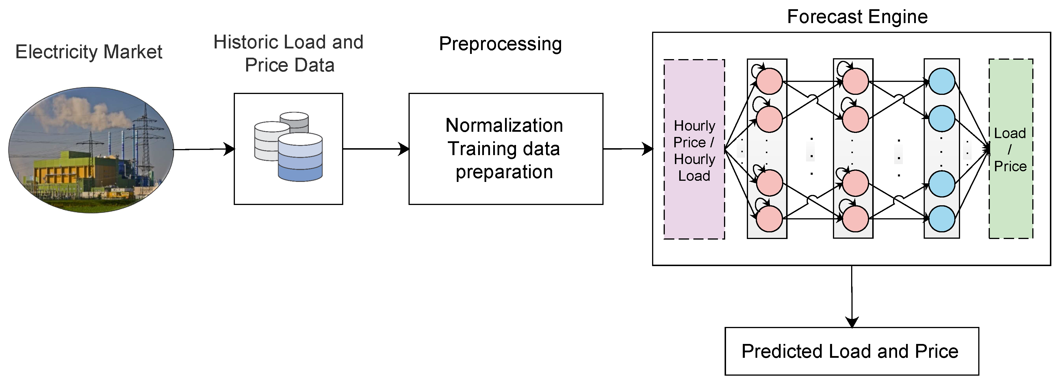
4. Proposed Model
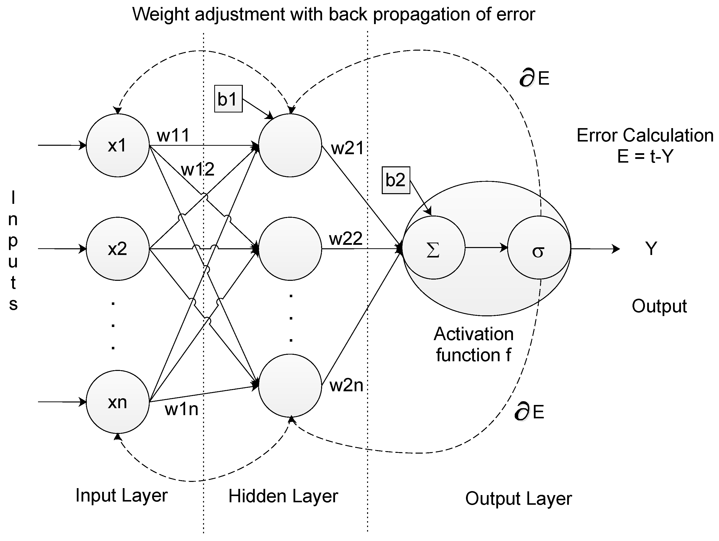
4.1. Artificial Neural Network
4.2. ANN for Time Series Forecasting
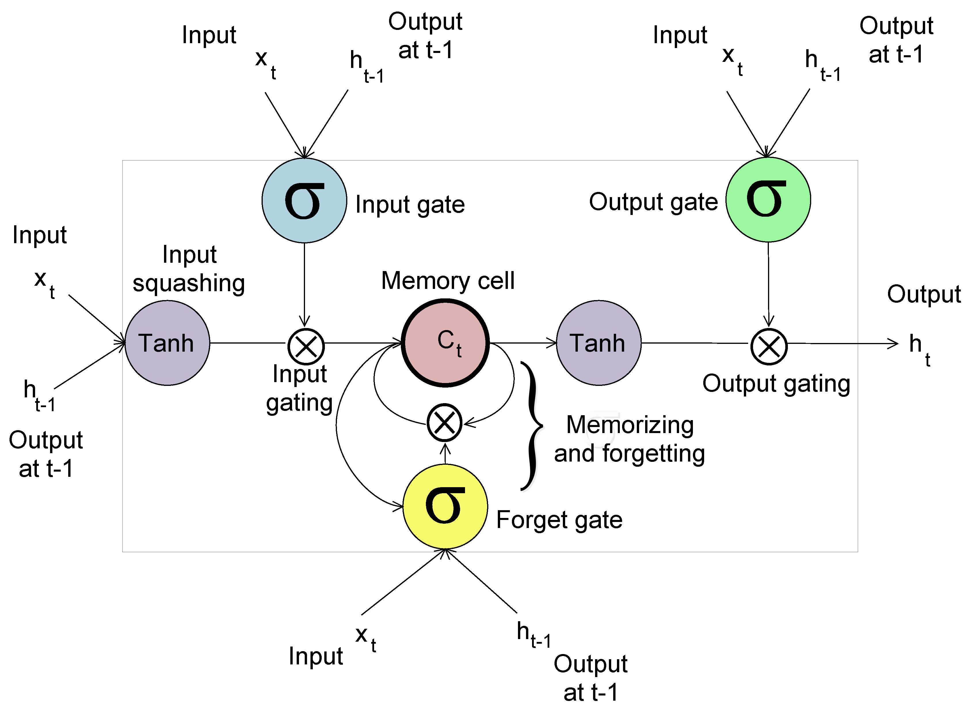
4.3. Long Short Term Memory
4.3.1. Forward Pass
4.3.2. Backward Pass
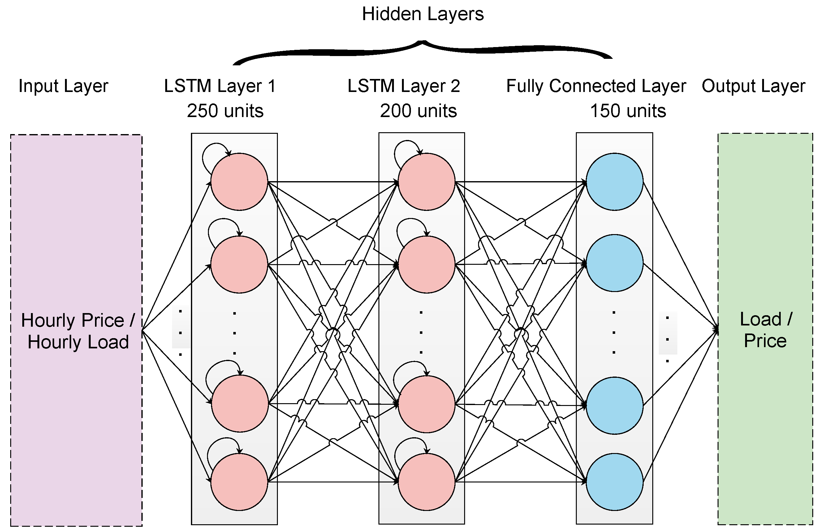
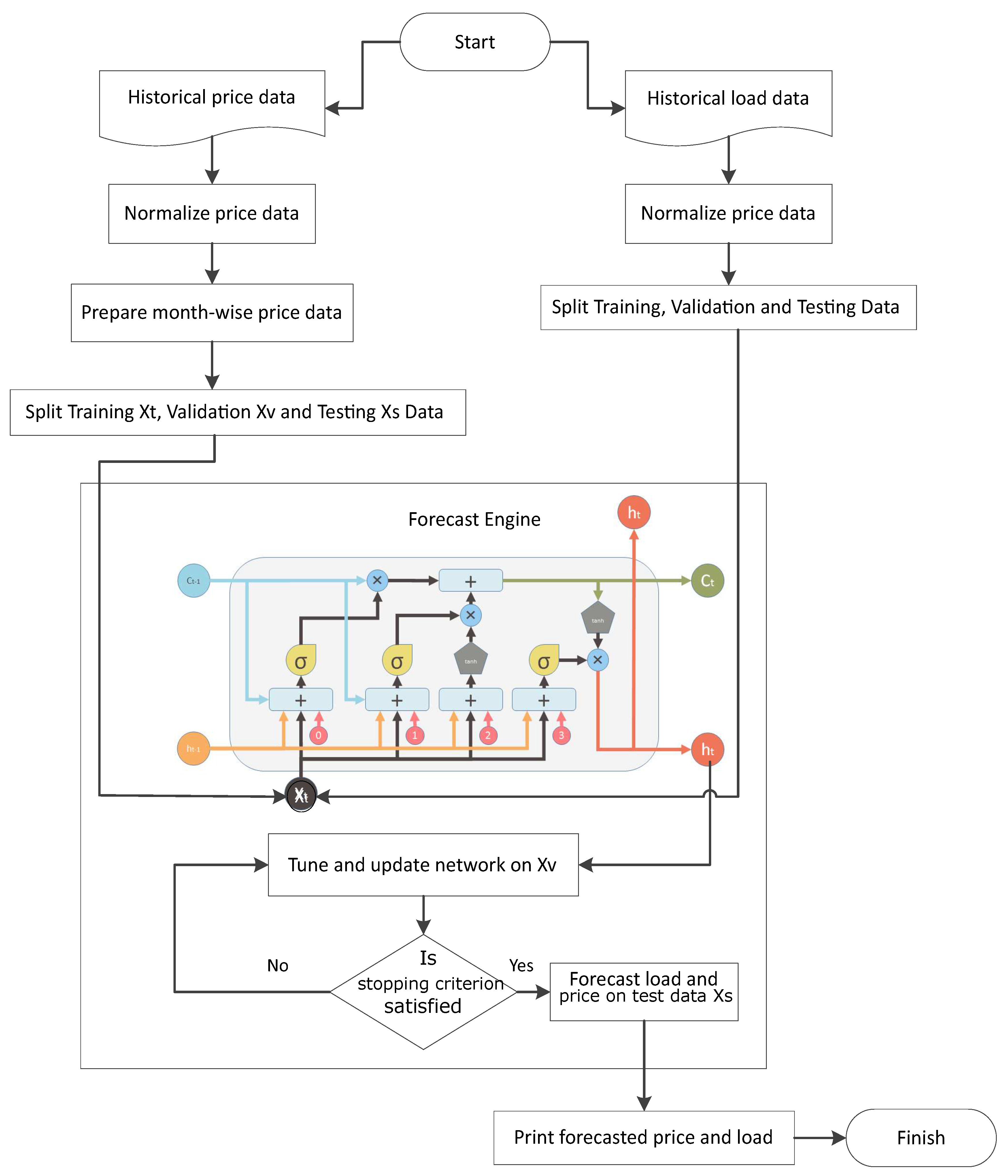
4.3.3. Deep LSTM
- Step 1: The historical price and load vectors are p and l, respectively, which are normalized as:where is vector of normalized price, is the function to calculate average and is the function to calculate standard deviation. This normalization is known as zero mean unit variance normalization. Price data are split month-wise. Data are divided into three partitions: train, validate and test.
- Step 2: Network is trained on training data and tested on validation data. NRMSE is calculated on validation data.
- Step 3: Network is tuned and updated on actual values of validation data.
- Step 4: The upgraded network is tested on the test data where day ahead, week ahead and month ahead prices and load are forecasted. Forecaster’s performance is evaluated by calculating the NRMSE.
4.4. Data Preprocessing
4.5. Network Training and Forecasting
4.6. Implementation Details
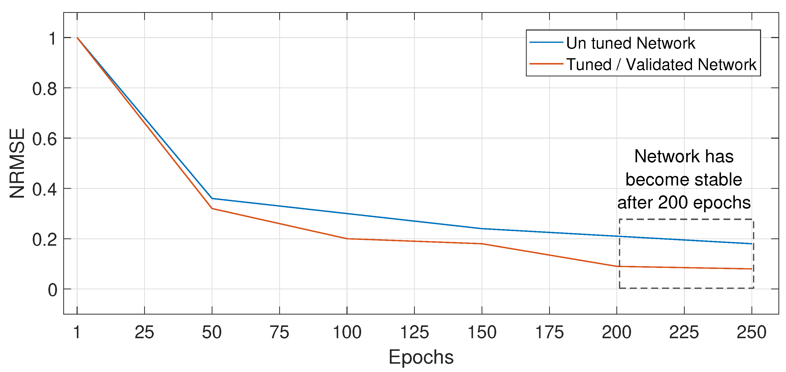
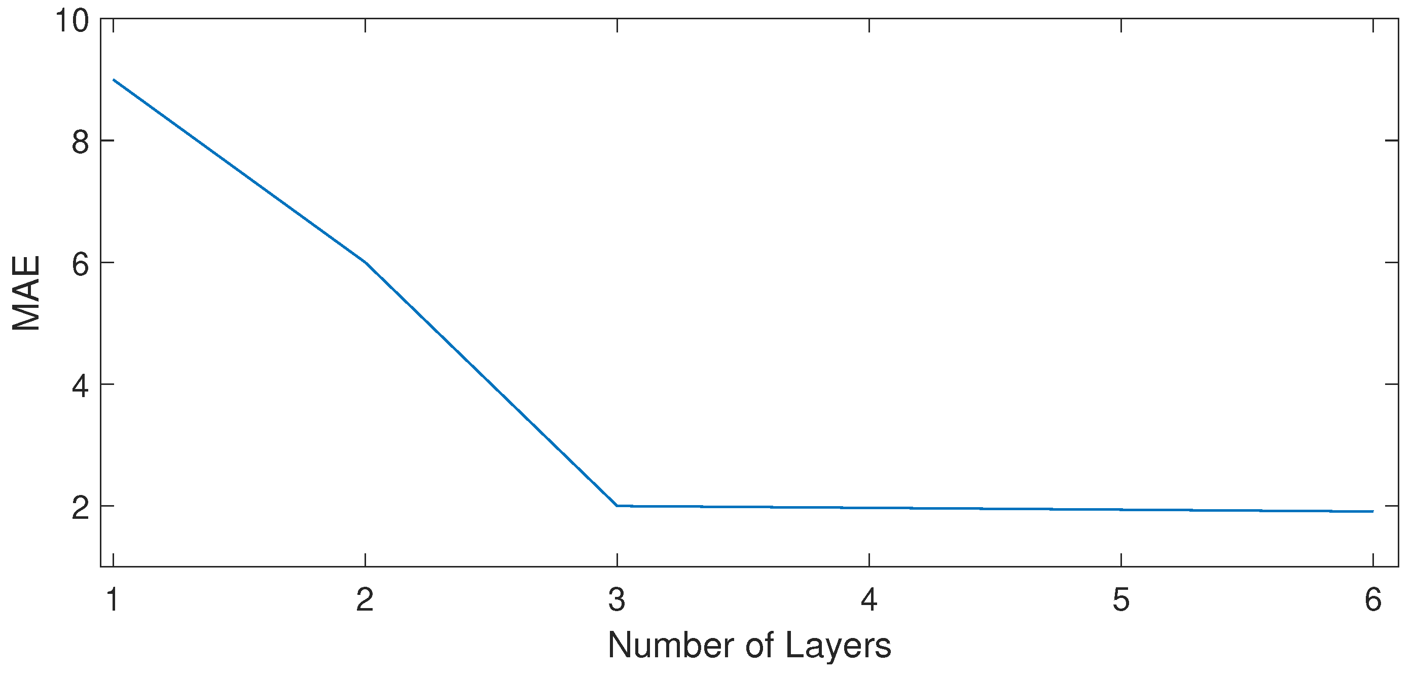
4.7. Network Stability
5. Results and Discussion
5.1. Working of DLSTM
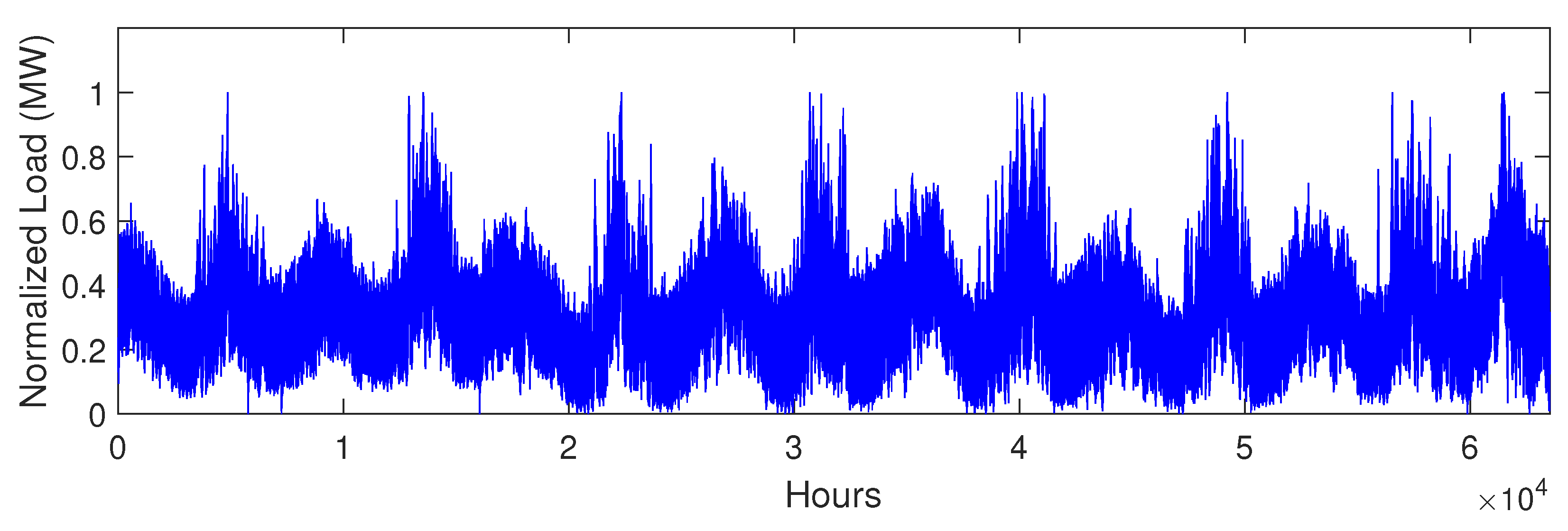
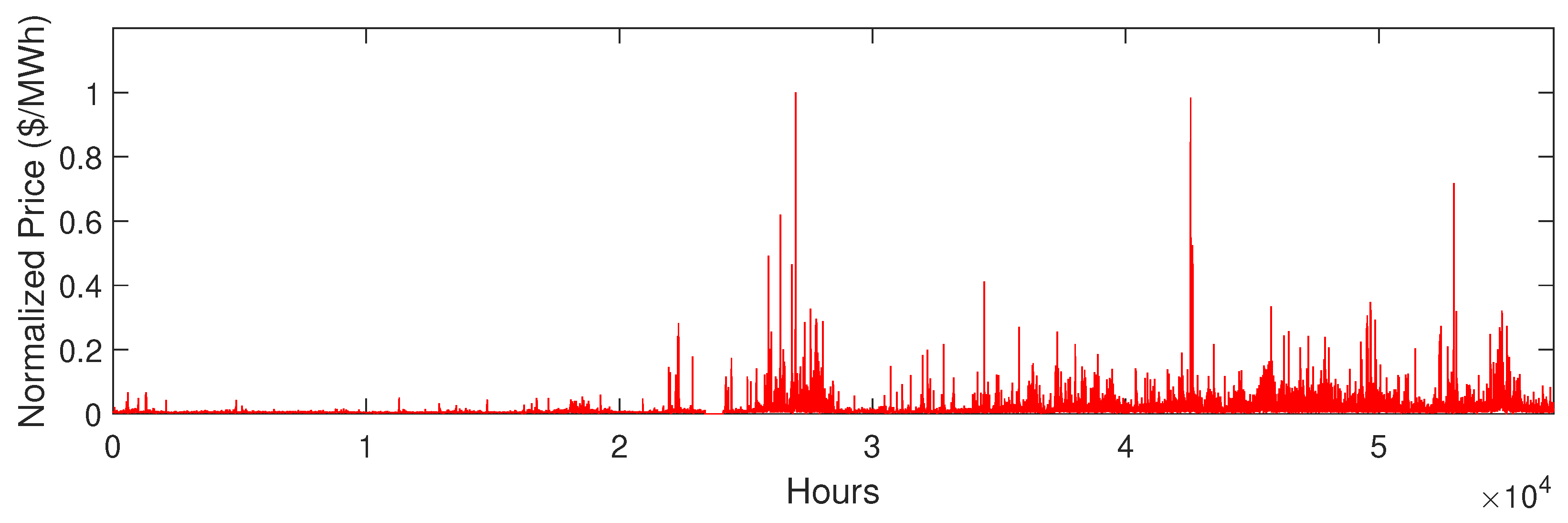
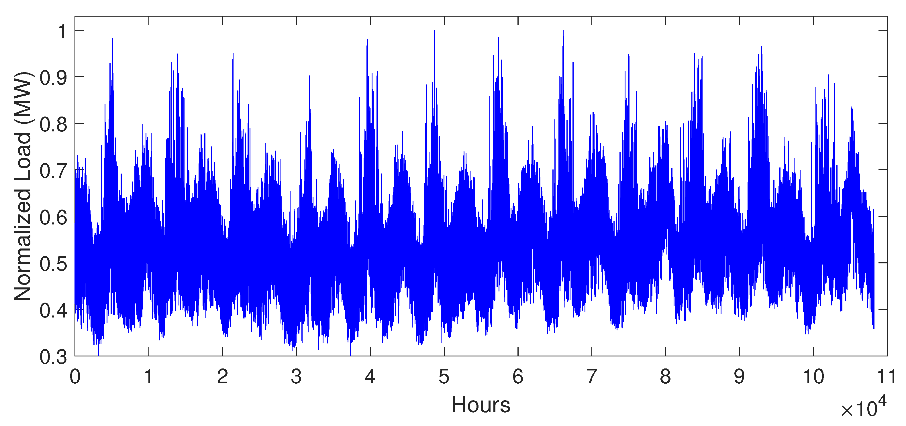
5.2. Data Description
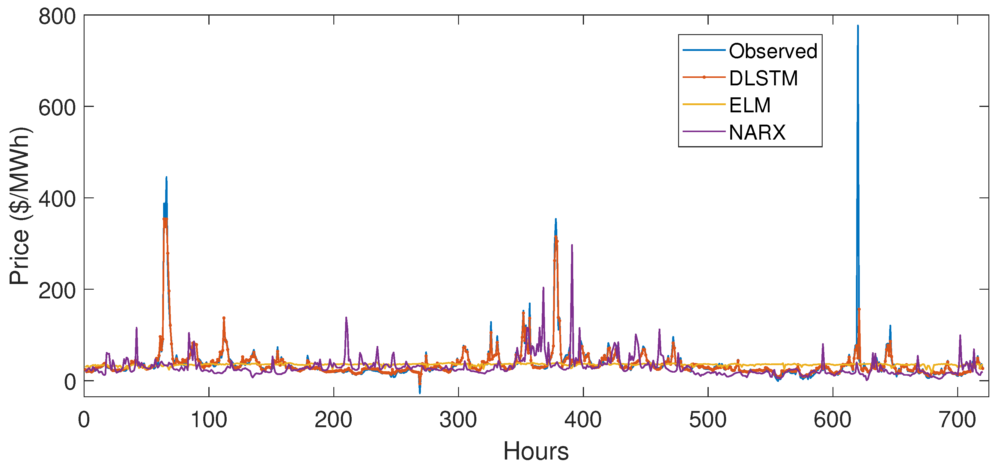
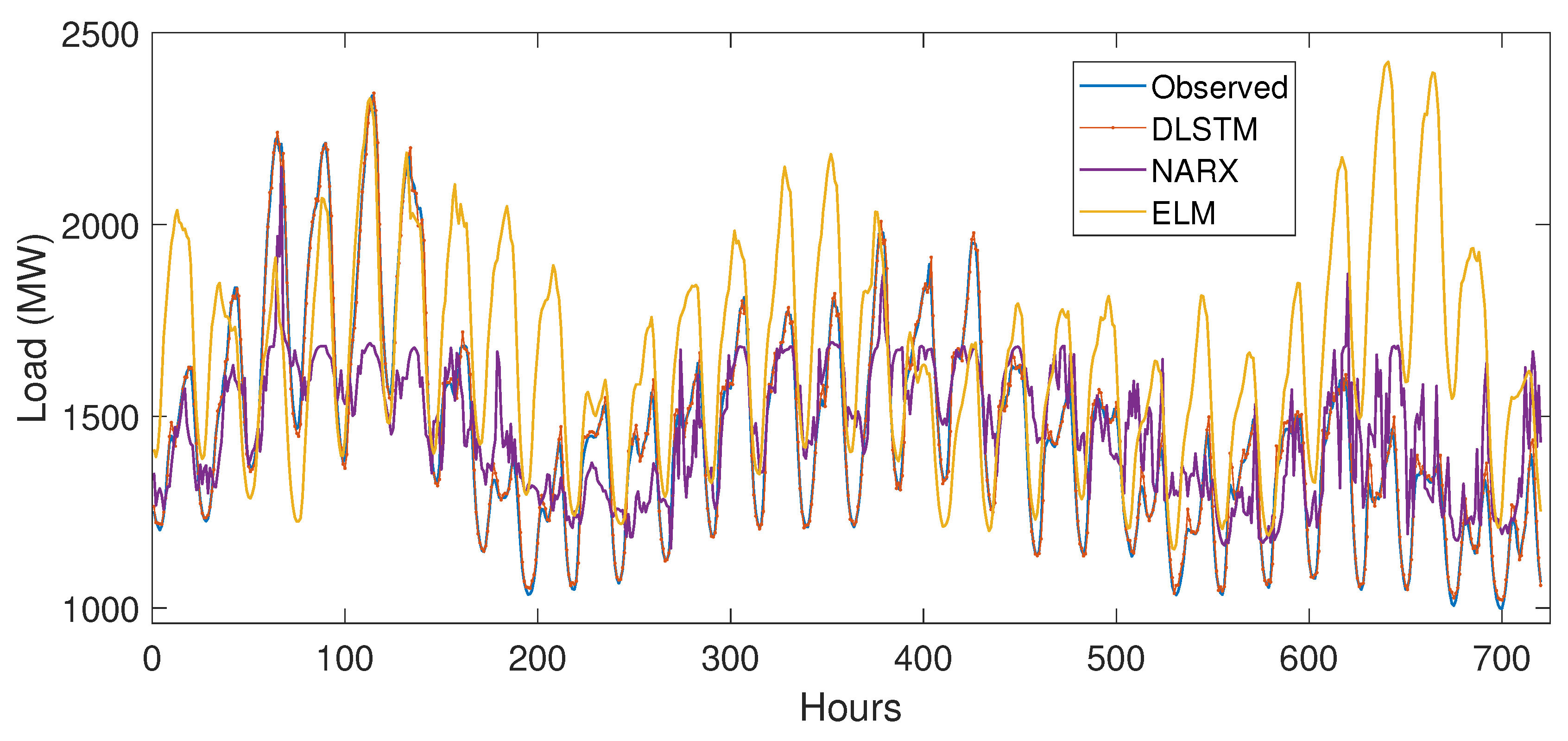
5.3. Simulation Results
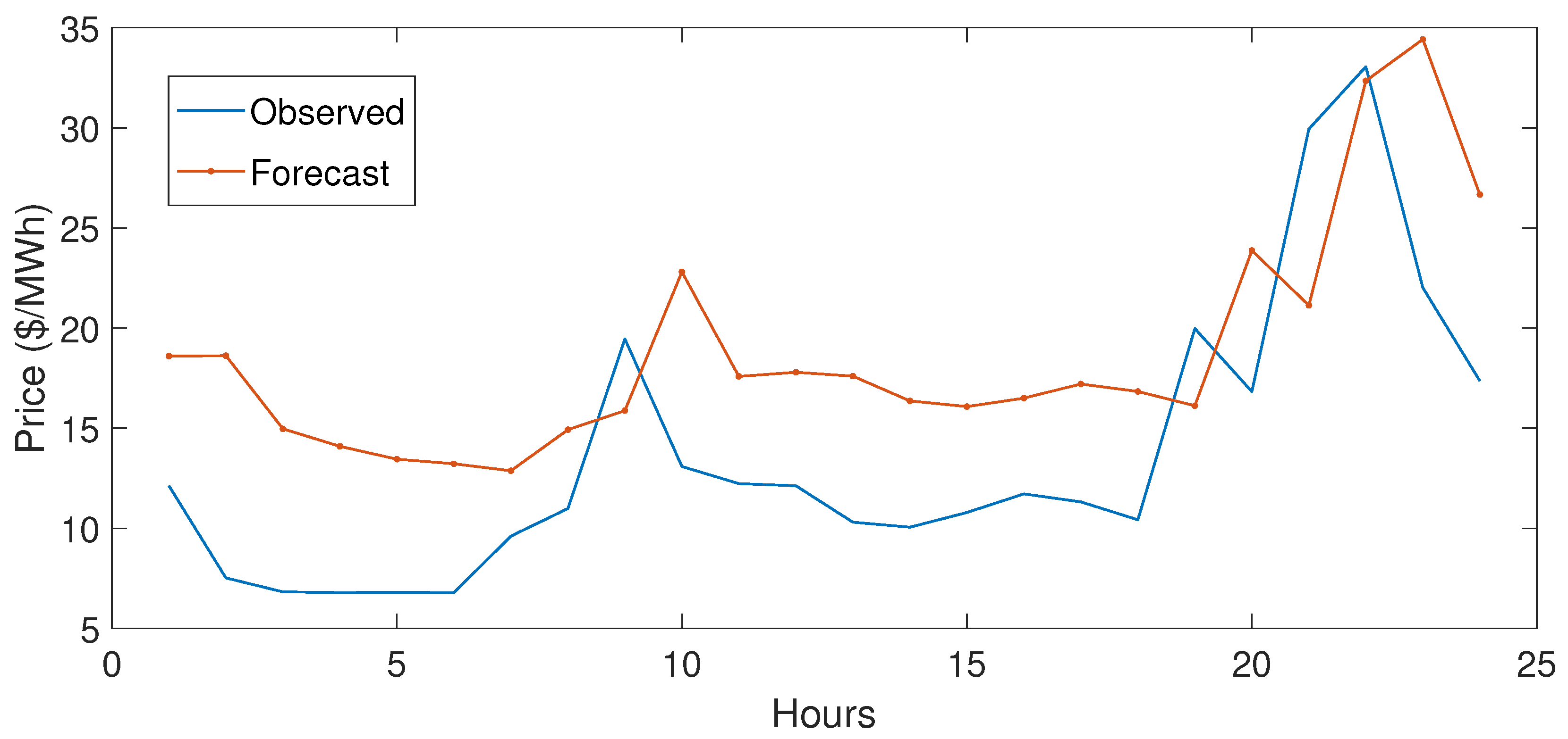
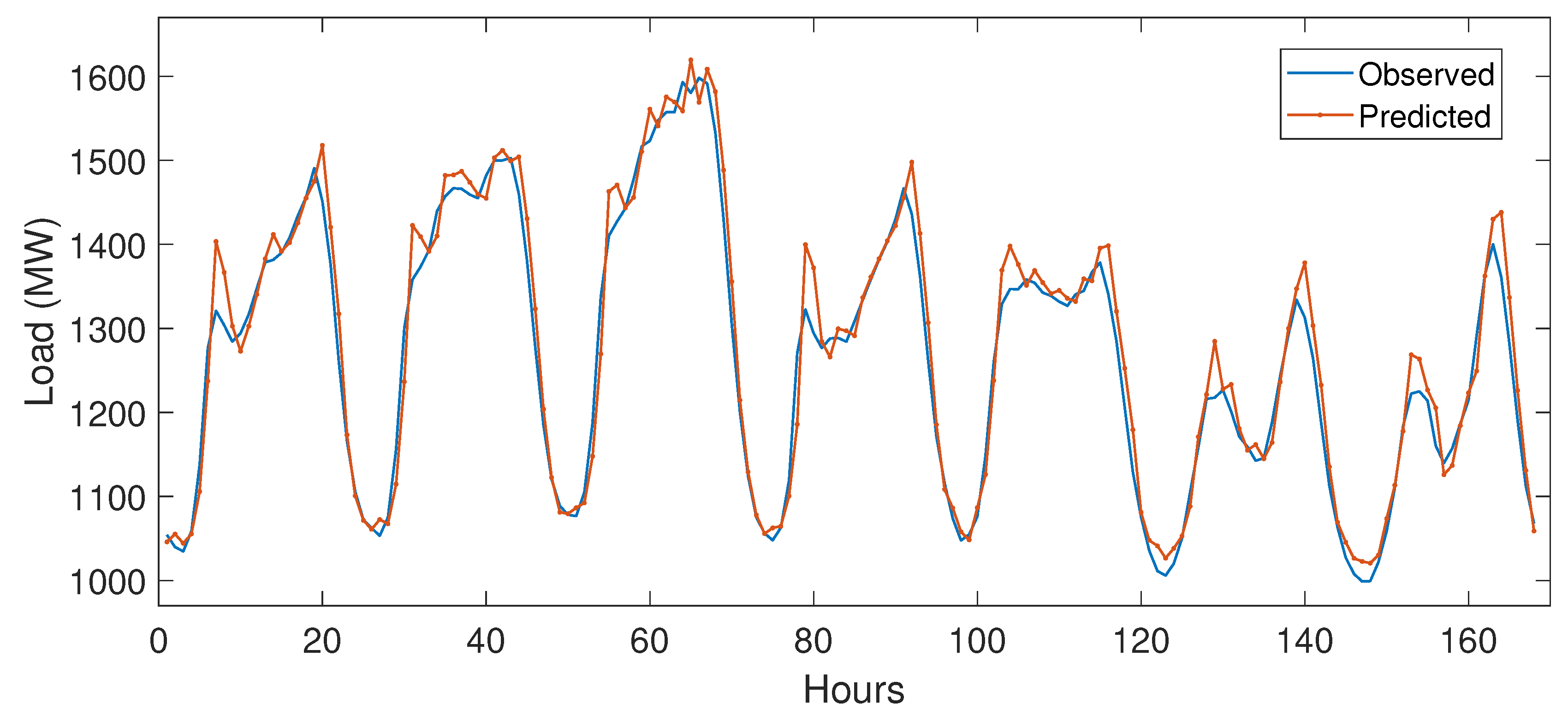
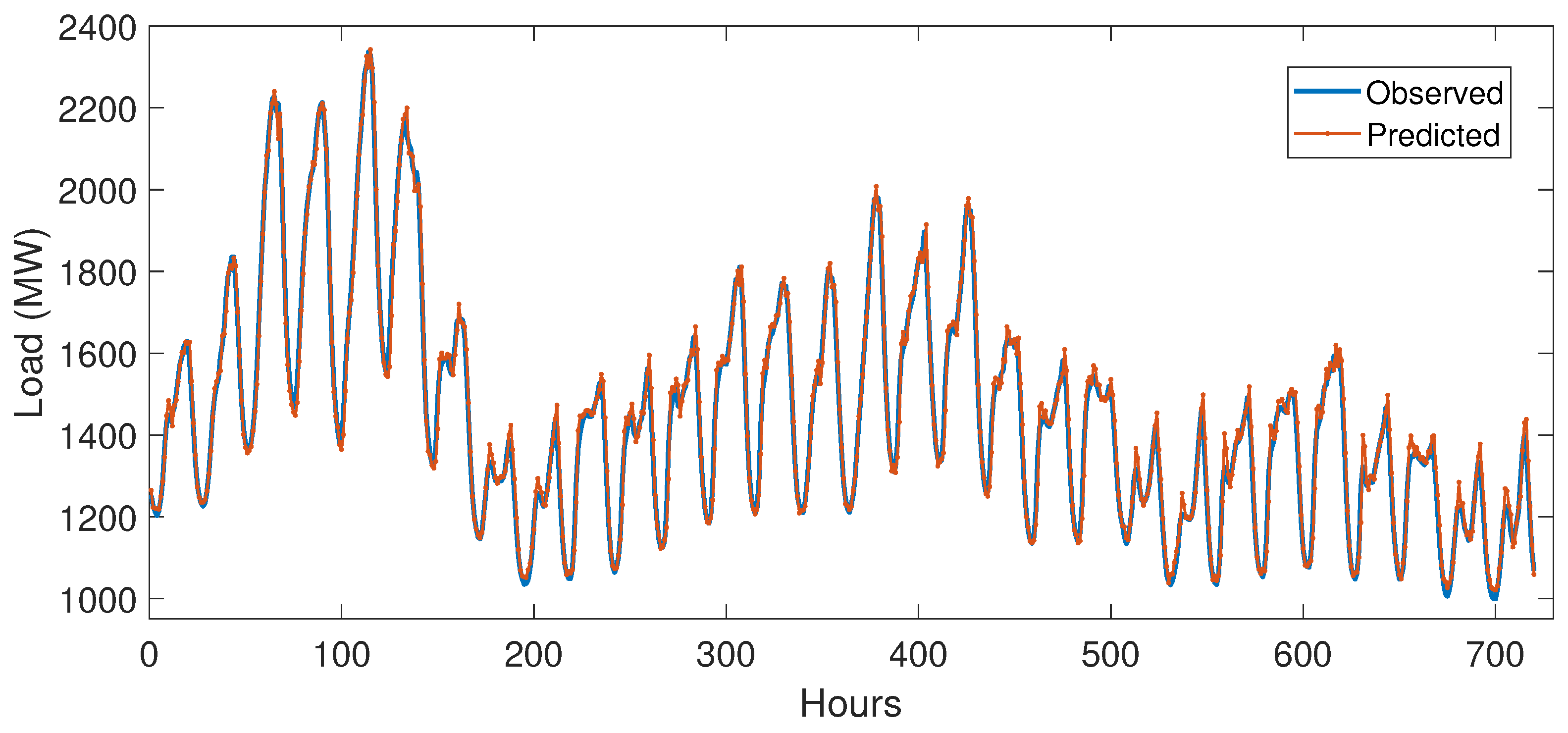
5.3.1. Case Study 1
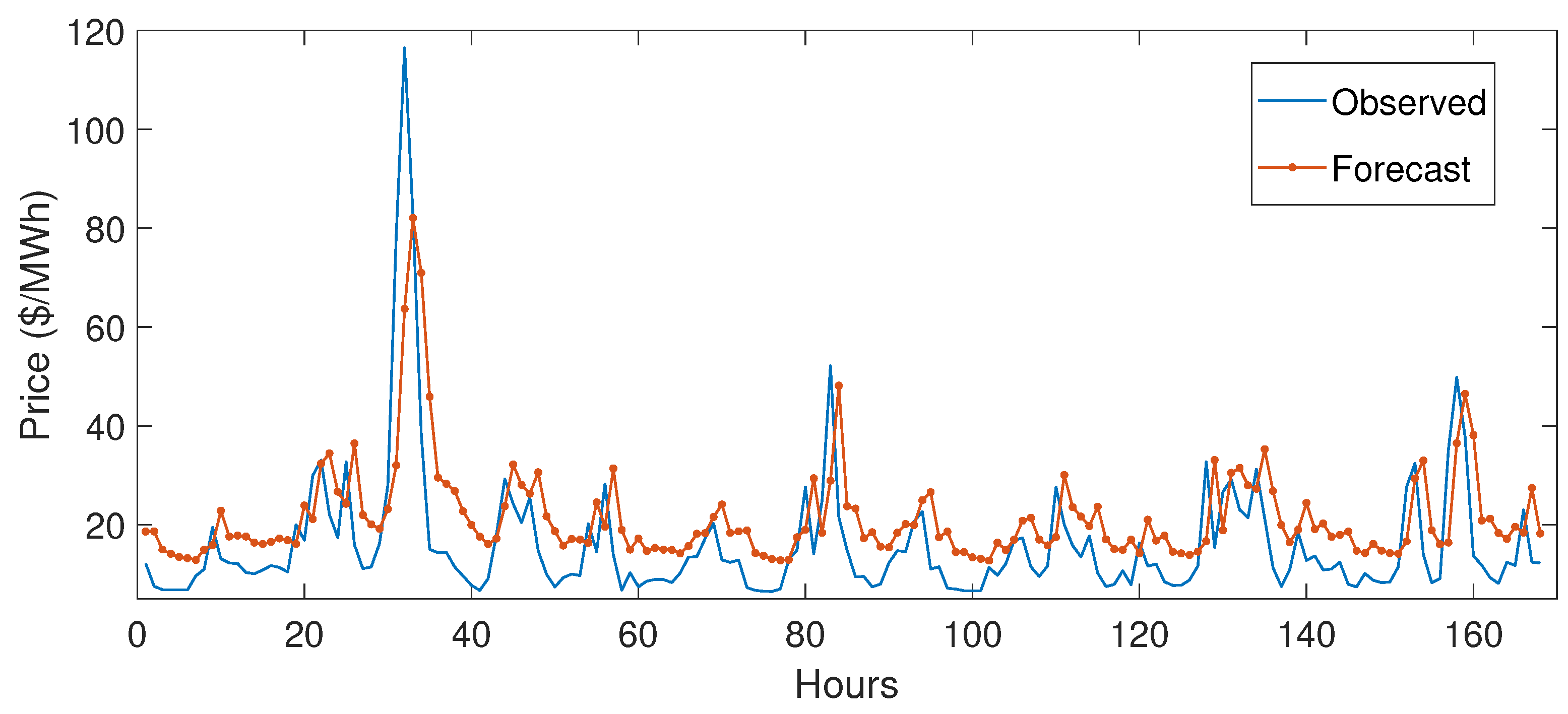
5.3.2. Case Study 2
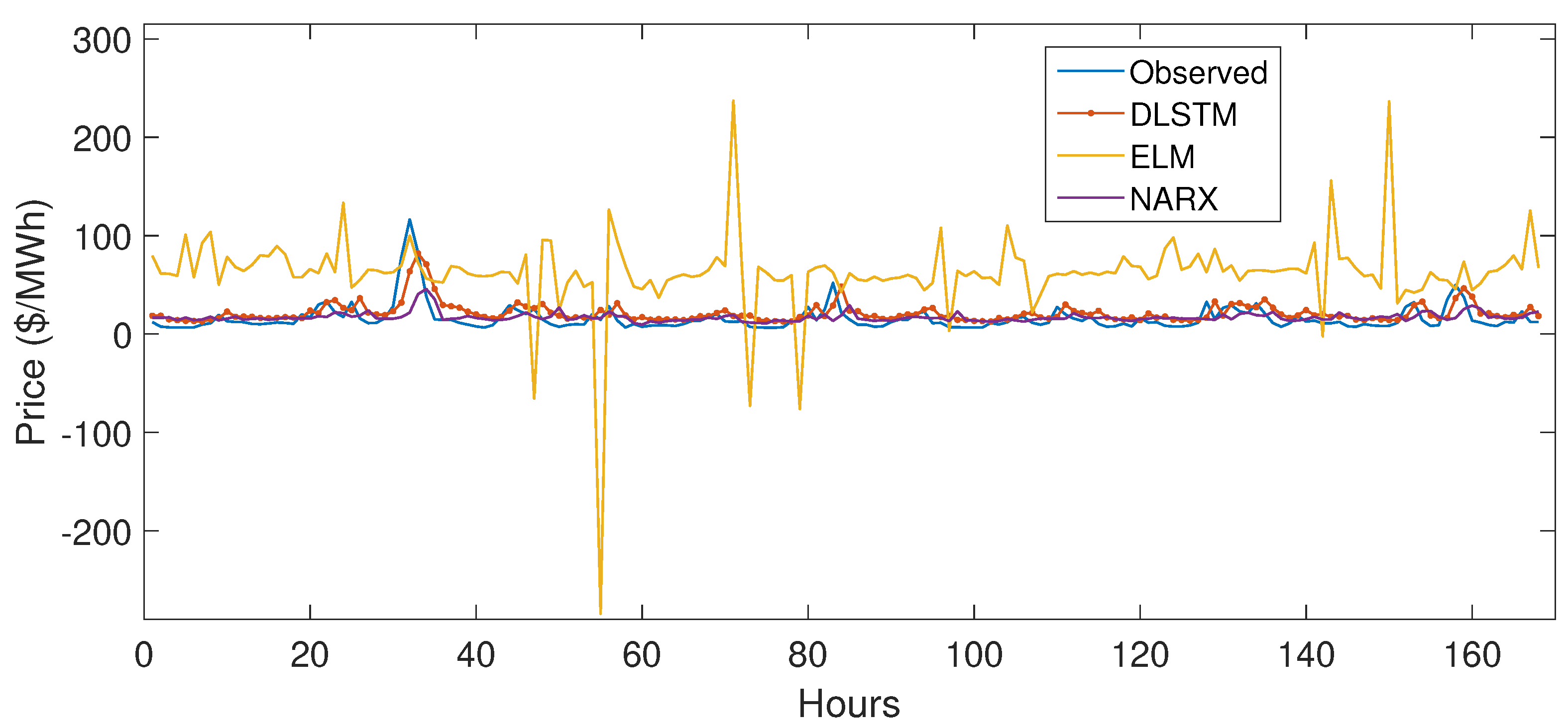
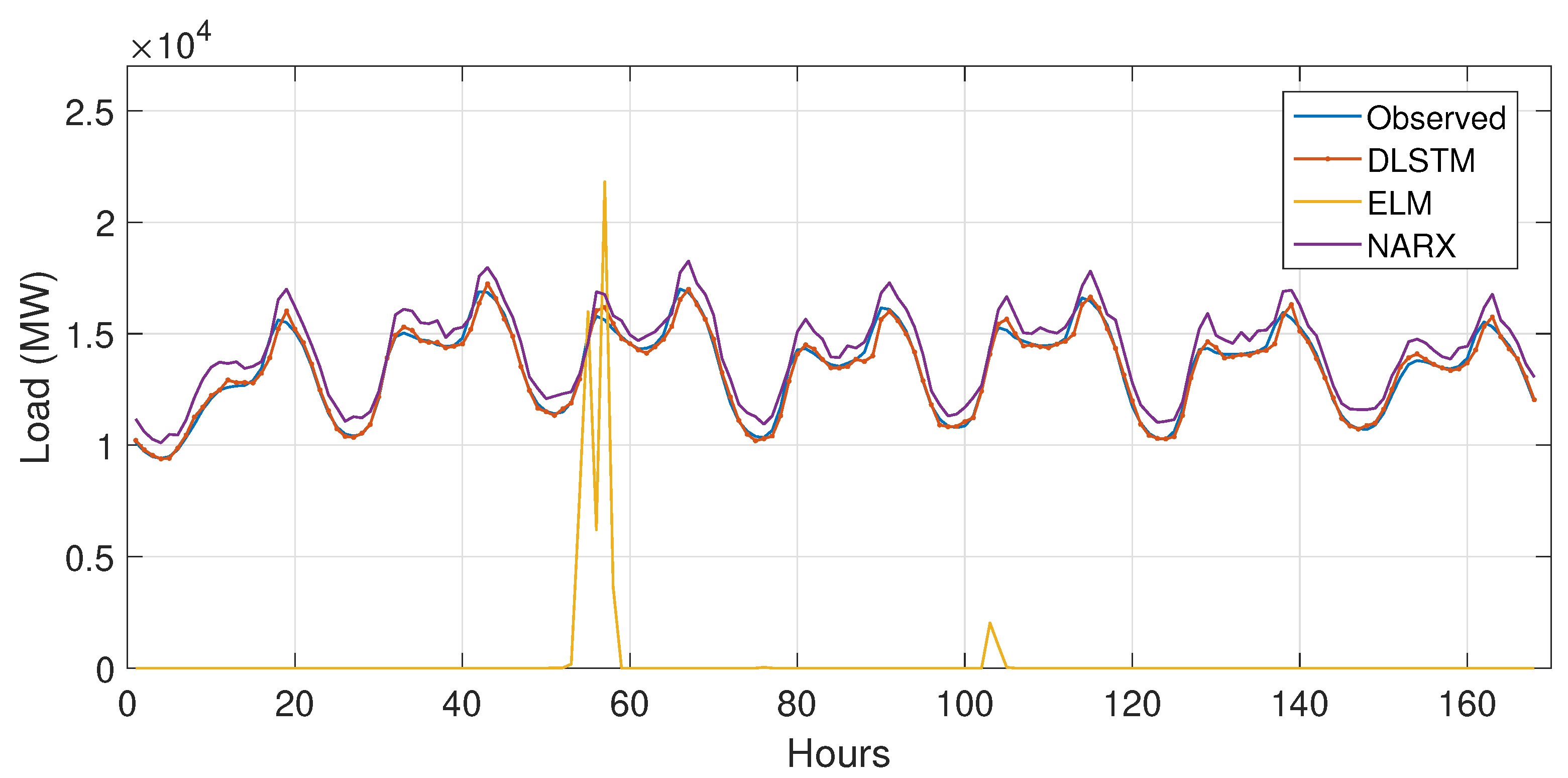
5.4. Performance Evaluation
6. Conclusions
Author Contributions
Acknowledgments
Conflicts of Interest
Abbreviations
| ABC | Artificial Bee Colony |
| AEMO | Australia Electricity Market Operators |
| ANN | Artificial Neural Networks |
| ARIMA | Auto-Regressive Integrated Moving Average |
| CNN | Convolution Neural Networks |
| CART | Classification and Regression Tree |
| DNN | Deep Neural Networks |
| DSM | Demand Side Management |
| DT | Decision Tree |
| DE | Differential Evaluation |
| DWT | Discrete Wavelet Transform |
| ELM | Extreme Learning Machine |
| GA | Genetic Algorithm |
| ISONE | Independent System Operator New England |
| KNN | K Nearest Neighbor |
| LSSVM | Least Square Support Vector Machine |
| LSTM | Long Short Term Memory |
| MAE | Mean Absolute Error |
| NYISO | New York Independent System Operator |
| NRMSE | Normalized Root Mean Square Error |
| RNN | Recurrent Neural Network |
| SAE | Stacked Auto-Encoders |
| STLF | Short-Term Load Forecast |
| SVM | Support Vector Machine |
| b | Bias |
| Current state of LSTM memory cell | |
| Error term of NARX | |
| Forget gate | |
| Input gate | |
| x | Input vector to network |
| Learning rate | |
| l | Load vector |
| Logistic sigmoid function | |
| LSTM memory cell | |
| LSTM memory cell’s input to itself | |
| Network weights | |
| y | Network output or forecasted value |
| M | Components of the training vector |
| n | Number of hidden units in ELM |
| Output gate | |
| Output of the ith hidden neuron | |
| p | Price vector |
| E | Squared error |
| T | Time step |
References
- Li, C.; Yu, X.; Yu, W.; Chen, G.; Wang, J. Efficient computation for sparse load shifting in demand side management. IEEE Trans. Smart Grid 2017, 8, 250–261. [Google Scholar] [CrossRef]
- Khan, A.R.; Mahmood, A.; Safdar, A.; Khan, Z.A.; Khan, N.A. Load forecasting, dynamic pricing and DSM in smart grid: A review. Renew. Sustain. Energy Rev. 2016, 54, 1311–1322. [Google Scholar] [CrossRef]
- Wang, D.; Luo, H.; Grunder, O.; Lin, Y.; Guo, H. Multi-step ahead electricity price forecasting using a hybrid model based on two-layer decomposition technique and BP neural network optimized by firefly algorithm. Appl. Energy 2017, 190, 390–407. [Google Scholar] [CrossRef]
- Gao, W.; Darvishan, A.; Toghani, M.; Mohammadi, M.; Abedinia, O.; Ghadimi, N. Different states of multi-block based forecast engine for price and load prediction. Int. J. Electr. Power Energy Syst. 2019, 104, 423–435. [Google Scholar] [CrossRef]
- Wang, K.; Wang, Y.; Hu, X.; Sun, Y.; Deng, D.J.; Vinel, A.; Zhang, Y. Wireless big data computing in smart grid. IEEE Wirel. Commun. 2017, 24, 58–64. [Google Scholar] [CrossRef]
- Zhou, K.; Fu, C.; Yang, S. Big data driven smart energy management: From big data to big insights. Renew. Sustain. Energy Rev. 2016, 56, 215–225. [Google Scholar] [CrossRef]
- Wang, K.; Yu, J.; Yu, Y.; Qian, Y.; Zeng, D.; Guo, S.; Xiang, Y.; Wu, J. A survey on energy internet: Architecture, approach, and emerging technologies. IEEE Syst. J. 2018, 12, 2403–2416. [Google Scholar] [CrossRef]
- Jiang, H.; Wang, K.; Wang, Y.; Gao, M.; Zhang, Y. Energy big data: A survey. IEEE Access 2016, 4, 3844–3861. [Google Scholar] [CrossRef]
- Mujeeb, S.; Javaid, N.; Akbar, M.; Khalid, R.; Nazeer, O.; Khan, M. Big Data Analytics for Price and Load Forecasting in Smart Grids. In Proceedings of the International Conference on Broadband and Wireless Computing, Communication and Applications, Taichung, Taiwan, 27–29 October 2018; Springer: Cham, Switzerland, 2018; pp. 77–87. [Google Scholar]
- Nadeem, Z.; Javaid, N.; Malik, A.W.; Iqbal, S. Scheduling appliances with GA, TLBO, FA, OSR and their hybrids using chance constrained optimization for smart homes. Energies 2018, 11, 888. [Google Scholar] [CrossRef]
- Naz, M.; Iqbal, Z.; Javaid, N.; Khan, Z.A.; Abdul, W.; Almogren, A.; Alamri, A. Efficient Power Scheduling in Smart Homes Using Hybrid Grey Wolf Differential Evolution Optimization Technique with Real Time and Critical Peak Pricing Schemes. Energies 2018, 11, 384. [Google Scholar] [CrossRef]
- Fan, S.K.S.; Su, C.J.; Nien, H.T.; Tsai, P.F.; Cheng, C.Y. Using machine learning and big data approaches to predict travel time based on historical and real-time data from Taiwan electronic toll collection. Soft Comput. 2018, 22, 5707–5718. [Google Scholar] [CrossRef]
- Liu, J.P.; Li, C.L. The short-term power load forecasting based on sperm whale algorithm and wavelet least square support vector machine with DWT-IR for feature selection. Sustainability 2017, 9, 1188. [Google Scholar] [CrossRef]
- Wang, F.; Li, K.; Zhou, L.; Ren, H.; Contreras, J.; Shafie-khah, M.; Catalao, J.P. Daily pattern prediction based classification modeling approach for day-ahead electricity price forecasting. Int. J. Electr. Power Energy Syst. 2019, 105, 529–540. [Google Scholar] [CrossRef]
- Fan, G.F.; Peng, L.L.; Zhao, X.; Hong, W.C. Applications of hybrid EMD with PSO and GA for an SVR-based load forecasting model. Energies 2017, 10, 1713. [Google Scholar] [CrossRef]
- Li, L.L.; Zhang, X.B.; Tseng, M.L.; Lim, M.; Han, Y. Sustainable energy saving: A junction temperature numerical calculation method for power insulated gate bipolar transistor module. J. Clean. Prod. 2018, 185, 198–210. [Google Scholar] [CrossRef]
- Fan, G.F.; Peng, L.L.; Hong, W.C.; Sun, F. Electric load forecasting by the SVR model with differential empirical mode decomposition and auto regression. Neurocomputing 2016, 173, 958–970. [Google Scholar] [CrossRef]
- Ghasemi, A.; Shayeghi, H.; Moradzadeh, M.; Nooshyar, M. A novel hybrid algorithm for electricity price and load forecasting in smart grids with demand-side management. Appl. Energy 2016, 177, 40–59. [Google Scholar] [CrossRef]
- Li, M.W.; Geng, J.; Hong, W.C.; Zhang, Y. Hybridizing chaotic and quantum mechanisms and fruit fly optimization algorithm with least squares support vector regression model in electric load forecasting. Energies 2018, 11, 2226. [Google Scholar] [CrossRef]
- Fan, G.F.; Peng, L.L.; Hong, W.C. Short term load forecasting based on phase space reconstruction algorithm and bi-square kernel regression model. Appl. Energy 2018, 224, 13–33. [Google Scholar] [CrossRef]
- Wang, K.; Xu, C.; Zhang, Y.; Guo, S.; Zomaya, A. Robust big data analytics for electricity price forecasting in the smart grid. IEEE Trans. Big Data 2017. [Google Scholar] [CrossRef]
- Ahmad, A.; Javaid, N.; Guizani, M.; Alrajeh, N.; Khan, Z.A. An accurate and fast converging short-term load forecasting model for industrial applications in a smart grid. IEEE Trans. Ind. Inform. 2017, 13, 2587–2596. [Google Scholar] [CrossRef]
- Rafiei, M.; Niknam, T.; Khooban, M.H. Probabilistic forecasting of hourly electricity price by generalization of ELM for usage in improved wavelet neural network. IEEE Trans. Ind. Inform. 2017, 13, 71–79. [Google Scholar] [CrossRef]
- Ahmad, A.; Javaid, N.; Alrajeh, N.; Khan, Z.A.; Qasim, U.; Khan, A. A modified feature selection and artificial neural network-based day-ahead load forecasting model for a smart grid. Appl. Sci. 2015, 5, 1756–1772. [Google Scholar] [CrossRef]
- Fan, C.; Xiao, F.; Zhao, Y. A short-term building cooling load prediction method using deep learning algorithms. Appl. Energy 2017, 195, 222–233. [Google Scholar] [CrossRef]
- Ryu, S.; Noh, J.; Kim, H. Deep neural network based demand side short term load forecasting. Energies 2016, 10, 3. [Google Scholar] [CrossRef]
- Tong, C.; Li, J.; Lang, C.; Kong, F.; Niu, J.; Rodrigues, J.J. An efficient deep model for day-ahead electricity load forecasting with stacked denoising auto-encoders. J. Parallel Distrib. Comput. 2017, 117, 267–273. [Google Scholar] [CrossRef]
- Ye, C.J. Electric Load Data Characterizing and Forecasting Based on Trend Index and Auto-Encoders. J. Eng. 2018, 2018, 1915–1921. [Google Scholar] [CrossRef]
- Shi, H.; Xu, M.; Li, R. Deep learning for household load forecasting—A novel pooling deep RNN. IEEE Trans. Smart Grid 2018, 9, 5271–5280. [Google Scholar] [CrossRef]
- Bouktif, S.; Fiaz, A.; Ouni, A.; Serhani, M. Optimal deep learning lstm model for electric load forecasting using feature selection and genetic algorithm: Comparison with machine learning approaches. Energies 2018, 11, 1636. [Google Scholar] [CrossRef]
- Ugurlu, U.; Oksuz, I.; Tas, O. Electricity Price Forecasting Using Recurrent Neural Networks. Energies 2018, 11, 1255. [Google Scholar] [CrossRef]
- Kuo, P.H.; Huang, C.J. An Electricity Price Forecasting Model by Hybrid Structured Deep Neural Networks. Sustainability 2018, 10, 1280. [Google Scholar] [CrossRef]
- Lago, J.; De Ridder, F.; De Schutter, B. Forecasting spot electricity prices: Deep learning approaches and empirical comparison of traditional algorithms. Appl. Energy 2018, 221, 386–405. [Google Scholar] [CrossRef]
- Moghaddass, R.; Wang, J. A hierarchical framework for smart grid anomaly detection using large-scale smart meter data. IEEE Trans. Smart Grid 2017. [Google Scholar] [CrossRef]
- Hou, W.; Ning, Z.; Guo, L.; Zhang, X. Temporal, functional and spatial big data computing framework for large-scale smart grid. IEEE Trans. Emerg. Top. Comput. 2017. [Google Scholar] [CrossRef]
- Perez-Chacon, R.; Luna-Romera, J.M.; Troncoso, A.; Martinez-Alvarez, F.; Riquelme, J.C. Big Data Analytics for Discovering Electricity Consumption Patterns in Smart Cities. Energies 2018, 11, 683. [Google Scholar] [CrossRef]
- Grolinger, K.; LHeureux, A.; Capretz, M.A.; Seewald, L. Energy forecasting for event venues: Big data and prediction accuracy. Energy Build. 2016, 112, 222–233. [Google Scholar] [CrossRef]
- Wang, P.; Liu, B.; Hong, T. Electric load forecasting with recency effect: A big data approach. Int. J. Forecast. 2016, 32, 585–597. [Google Scholar] [CrossRef]
- Zhang, Q.; Yang, L.T.; Chen, Z.; Li, P. A survey on deep learning for big data. Inf. Fusion 2018, 42, 146–157. [Google Scholar] [CrossRef]
- ISO NE Electricity Market Data. Available online: https://www.iso-ne.com/isoexpress/web/reports/pricing/-/tree/zone-info (accessed on 25 November 2018).
- NYISO Market Operations Data. Available online: http://www.nyiso.com/public/markets_operations/market_data/custom_report (accessed on 25 November 2018).
- Rosenblatt, F. Principles of Neurodynamics: Perceptrons and the Theory of Brain Mechanisms; Spartan Books: Washington, DC, USA, 1961. [Google Scholar]
- Hochreiter, S.; Schmidhuber, J. Long short-term memory. Neural Comput. 1997, 9, 1735–1780. [Google Scholar] [CrossRef]
- Manic, M.; Amarasinghe, K.; Rodriguez-Andina, J.J.; Rieger, C. Intelligent buildings of the future: Cyberaware, deep learning powered, and human interacting. IEEE Ind. Electron. Mag. 2016, 10, 32–49. [Google Scholar] [CrossRef]
- Krueger, D.; Memisevic, R. Regularizing RNNs by stabilizing activations. arXiv, 2015; arXiv:1511.08400. [Google Scholar]
- Yang, Z.; Ce, L.; Lian, L. Electricity price forecasting by a hybrid model, combining wavelet transform, ARMA and kernel-based extreme learning machine methods. Appl. Energy 2017, 190, 291–305. [Google Scholar] [CrossRef]
- Buitrago, J.; Asfour, S. Short-term forecasting of electric loads using nonlinear autoregressive artificial neural networks with exogenous vector inputs. Energies 2017, 10, 40. [Google Scholar] [CrossRef]
- Derrac, J.; Garcia, S.; Molina, D.; Herrera, F. A practical tutorial on the use of nonparametric statistical tests as a methodology for comparing evolutionary and swarm intelligence algorithms. Swarm Evol. Comput. 2015, 1, 3–18. [Google Scholar] [CrossRef]
- Martin, P.; Moreno, G.; Rodriguez, F.; Jimenez, J.; Fernandez, I. A Hybrid Approach to Short-Term Load Forecasting Aimed at Bad Data Detection in Secondary Substation Monitoring Equipment. Sensors 2018, 18, 3947. [Google Scholar] [CrossRef] [PubMed]
- Diebold, F.X.; Mariano, R.S. Comparing predictive accuracy. J. Bus. Econ. Stat. 2002, 20, 134–144. [Google Scholar] [CrossRef]
- Ludwig, N.; Feuerriegel, S.; Neumann, D. Putting Big Data analytics to work: Feature selection for forecasting electricity prices using the LASSO and random forests. J. Decis. Syst. 2015, 24, 19–36. [Google Scholar] [CrossRef]


| Task | Forecast Horizon | Platform/Testbed | Dataset | Algorithms |
|---|---|---|---|---|
| Load forecasting [13] | Short-term | Hourly data of 6 states OF USA | NYISO 2015 | DWT-IR, SVM, Sperm whale algorithm |
| Load forecasting [14] | Short-term | Hourly price of PJM | PJM, 2016–2017 | Weighted voting mechanism |
| Load and price forecasting [18] | Short-term | Hourly data New South Wales, New York | NYISO, PJM, AEMO, 2012, 2014, 2010 | FWPT, NLSSVM, ARIMA, ABC |
| Price forecasting [21] | Short-term | Hourly data of 6 states of USA | ISO NE, 2010–2015 | GCA, Random forest, ReliefF, DE-SVM |
| Load forecasting [22] | Short-term | Electricity market of three USA grids: FE, DAYTOWN, and EKPC | PJM | Modified Mutual Information (MI), ANN |
| Price forecasting [23] | Short-term | Ontario electricity market | AEMO, 2014 | ELM based improved WNN |
| Load forecasting [24] | Short-term | Electricity market data of 3 USA grids | PJM, 2014 | Modified MI, ANN |
| Load forecasting [25] | Short-term | Half hour cooling consumption data of a educational building | Hong Kong, 2015 | Deep auto-encoders |
| Load forecasting [26] | Short-term | Korea | Korea Electric Power Company, 2012–2014 | DNN, RBM, ReLU |
| Load forecasting [27] | Short-term | Hourly load and weather data of four regions | Los Angeles, California, Florida and New York City, July 2015–August 2016 | Stacked de-noising auto-encoder, SVR |
| Load forecasting [28] | Short-term | 15 min consumption data | Single user high consumption data from Foshan, Guangdong province of China, March–May 2016 | Trend index, auto-encoder |
| Load forecasting [29] | Short-term | Ireland consumption | Load profiles database of Ireland | Pooling deep RNN |
| Load forecasting [30] | Medium-term | France | Half hourly metropolitan electricity load, 2008–2016 | LSTM, GA |
| Price forecasting [31] | Medium-term | Hourly load of 5 hubs of Midcontinent Independent System Operator (MISO) | MISO USA, 2012–2014 | Stacked de-noising autoencoder |
| Price forecasting [32] | Short-term | Hourly Turkish day-ahead electricity market | Turkey, 2013–2016 | Gated recurrent network |
| Price forecasting [33] | Short-term | Half hour regulation market capacity clearing price | Electric power markets (PJM), 2017 | CNN, LSTM |
| Load forecasting [36] | Short-term | Eight buildings of a public university | 15 min consumption, 2011–2017 | K-means clustering, Davies–Bouldin distance function |
| Consumption and peak demand forecasting [37] | Medium-term | Entertainment venues of Ontario | Daily, hourly and 15 min energy consumption, 2012–2014 | ANN, SVR |
| Demand forecasting [38] | Short-term | 21 zones of USA | Temperature, humidity and consumption data, 2004–2007 | Recency effect model without computational constraints |
| Data | ISO NE | NYISO | ||||||
|---|---|---|---|---|---|---|---|---|
| Month | January | February | March | April | January | February | March | April |
| MAE | 1.72 | 1.45 | 2.7 | 1.92 | 3.6 | 3.8 | 2.9 | 2.7 |
| NRMSE | 0.076 | 0.062 | 0.102 | 0.082 | 0.032 | 0.043 | 0.037 | 0.047 |
| Month | May | June | July | August | May | June | July | August |
| MAE | 2.83 | 1.45 | 1.96 | 1.92 | 2.14 | 2.7 | 2.42 | 2.56 |
| NRMSE | 0.107 | 0.062 | 0.087 | 0.102 | 0.014 | 0.017 | 0.024 | 0.031 |
| Month | September | October | November | December | September | October | November | December |
| MAE | 2.04 | 1.36 | 2.01 | 1.98 | 2.19 | 2.36 | 2.8 | 2.12 |
| NRMSE | 0.093 | 0.057 | 0.124 | 0.115 | 0.047 | 0.014 | 0.018 | 0.021 |
| Forecast | Data | ISO NE | NYISO | ||
|---|---|---|---|---|---|
| Forecasting Method | MAE | NRMSE | MAE | NRMSE | |
| ELM | 67.4 | 11.86 | 9.97 | 7.36 | |
| Price Forecast | NARX | 12.47 | 8.24 | 10.32 | 8.62 |
| WT+SAPSO+KELM [46] | 8.99 | 0.13 | 19.26 | 0.06 | |
| DLSTM | 1.945 | 0.08 | 2.6 | 0.028 | |
| ELM | 52.8 | 8.42 | 9.68 | 5.24 | |
| Load Forecast | NARX | 37.18 | 14.74 | 12.36 | 11.57 |
| INARX [47] | 9.7 | 0.2 | 1.9 | 0.02 | |
| DLSTM | 2.9 | 0.087 | 1.4 | 0.012 | |
| Data | ISO NE | NYISO | |||
|---|---|---|---|---|---|
| Forecast | Forecasting Method | Diebold–Mariano | Friedman | Diebold–Mariano | Friedman |
| DLSTM vs. | F Rank | DLSTM vs. | F Rank | ||
| Price Forecast | ELM | 47.3 | 4 | 52.6 | 4 |
| NARX | 27.6 | 3 | 21.4 | 3 | |
| WT+SAPSO+KELM [46] | 12.8 | 2 | 8.6 | 2 | |
| DLSTM | N/A | 1 | N/A | 1 | |
| Load Forecast | ELM | 43.2 | 3 | 34.7 | 4 |
| NARX | 6.8 | 2 | 7.9 | 3 | |
| INARX [47] | 4.2 | 2 | 3.8 | 2 | |
| DLSTM | N/A | 1 | N/A | 1 | |
© 2019 by the authors. Licensee MDPI, Basel, Switzerland. This article is an open access article distributed under the terms and conditions of the Creative Commons Attribution (CC BY) license (http://creativecommons.org/licenses/by/4.0/).
Share and Cite
Mujeeb, S.; Javaid, N.; Ilahi, M.; Wadud, Z.; Ishmanov, F.; Afzal, M.K. Deep Long Short-Term Memory: A New Price and Load Forecasting Scheme for Big Data in Smart Cities. Sustainability 2019, 11, 987. https://doi.org/10.3390/su11040987
Mujeeb S, Javaid N, Ilahi M, Wadud Z, Ishmanov F, Afzal MK. Deep Long Short-Term Memory: A New Price and Load Forecasting Scheme for Big Data in Smart Cities. Sustainability. 2019; 11(4):987. https://doi.org/10.3390/su11040987
Chicago/Turabian StyleMujeeb, Sana, Nadeem Javaid, Manzoor Ilahi, Zahid Wadud, Farruh Ishmanov, and Muhammad Khalil Afzal. 2019. "Deep Long Short-Term Memory: A New Price and Load Forecasting Scheme for Big Data in Smart Cities" Sustainability 11, no. 4: 987. https://doi.org/10.3390/su11040987
APA StyleMujeeb, S., Javaid, N., Ilahi, M., Wadud, Z., Ishmanov, F., & Afzal, M. K. (2019). Deep Long Short-Term Memory: A New Price and Load Forecasting Scheme for Big Data in Smart Cities. Sustainability, 11(4), 987. https://doi.org/10.3390/su11040987