Article

Deep Long Short-Term Memory: A New Price and Load Forecasting Scheme for Big Data in Smart Cities

1
Department of Computer Science, COMSATS University Islamabad, Islamabad 44000, Pakistan
2
Department of Computer System Engineering, University of Engineering and Technology, Peshawar 25000, Pakistan
3
Department of Electronics and Communication Engineering, Kwangwoon University, Seoul 01897, Korea
4
Department of Computer Science, COMSATS University Islamabad, Wah Campus, Wah Cantonment 47040, Pakistan
*
Authors to whom correspondence should be addressed.
Sustainability 2019, 11(4), 987; https://doi.org/10.3390/su11040987
Submission received: 25 November 2018 / Revised: 9 January 2019 / Accepted: 25 January 2019 / Published: 14 February 2019
(This article belongs to the Special Issue Data Analytics on Sustainable, Resilient and Just Communities)

Abstract

:
This paper focuses on analytics of an extremely large dataset of smart grid electricity price and load, which is difficult to process with conventional computational models. These data are known as energy big data. The analysis of big data divulges the deeper insights that help experts in the improvement of smart grid’s (SG) operations. Processing and extracting of meaningful information from data is a challenging task. Electricity load and price are the most influential factors in the electricity market. For improving reliability, control and management of electricity market operations, an exact estimate of the day ahead load is a substantial requirement. Energy market trade is based on price. Accurate price forecast enables energy market participants to make effective and most profitable bidding strategies. This paper proposes a deep learning-based model for the forecast of price and demand for big data using Deep Long Short-Term Memory (DLSTM). Due to the adaptive and automatic feature learning mechanism of Deep Neural Network (DNN), the processing of big data is easier with LSTM as compared to the purely data-driven methods. The proposed model was evaluated using well-known real electricity markets’ data. In this study, day and week ahead forecasting experiments were conducted for all months. Forecast performance was assessed using Mean Absolute Error (MAE) and Normalized Root Mean Square Error (NRMSE). The proposed Deep LSTM (DLSTM) method was compared to traditional Artificial Neural Network (ANN) time series forecasting methods, i.e., Nonlinear Autoregressive network with Exogenous variables (NARX) and Extreme Learning Machine (ELM). DLSTM outperformed the compared forecasting methods in terms of accuracy. Experimental results prove the efficiency of the proposed method for electricity price and load forecasting.

1. Introduction

The Smart Grid (SG) is the modern and intelligent power grid that efficiently manages the generation, distribution and consumption of electricity. SG introduced communication, sensing and control technologies in power grids. It facilitates consumers in an economical, reliable, sustainable and secure manner. Consumers can manage their energy demand in an economical fashion based on Demand Side Management (DSM) [1]. The DSM program allows customers to manage their load demand according to the price variations. It offers energy consumers for load shifting and energy preservation in order to reduce the cost of power consumption. Smart grid establishes an interactive environment between energy consumers and utility. Customers partake in smart grid operations to reduce the price by load shifting and energy preservation.
Competitive electricity markets benefit from load and price forecast. Several important operating decisions are based on load forecasts, such as power generation scheduling, demand supply management, maintenance planning and reliability analysis [2].
Price forecast is crucial to energy market participants for bidding strategies formulation, assets allocation, risk assessment and facility investment planning. Effective bidding strategies help market participants in maximizing profit. Utility maximization is the ultimate goal of both power producers and consumers. With the help of a robust and exact price estimate, power producers can maximize profit and consumers can minimize the cost of their purchased electricity [3]. The necessity of efficient generation and consumption is another crucial issue in the energy sector. Most of the generated electricity cannot be stored, therefore, a perfect equilibrium is necessary to be maintained between the generated and consumed electricity. Therefore, an accurate forecast of both electricity load and price holds a great importance in market operations management.
ISO NE (Independent System Operator, New England) is a Regional Transmission Organization (RTO), coordinated by an ISO. It is responsible for management of the wholesale energy markets operations and power trade auctions. ISO NE provides energy to six states of New England including Connecticut, Maine, Massachusetts, New Hampshire, Rhodes Island and Vermont. In this study, analytics were performed on a large dataset of ISO NE and NYISO. Electricity price and load exhibit certain characteristics. Electricity load and price have a relationship of direct proportionality [4]. However, some unexpected variations are observed in the price data. There are various reasons for these unexpected changes in price pattern. In reality, the price is not only affected by the change in load. Several different parameters influence the energy price: fuel price, availability of inexpensive generation sources (e.g., photovoltaic generation, windmill generation, etc.), weather conditions, etc.
In this study, analyses were performed on a large amount of electricity data referred to as energy big data. Big data are defined as datasets with extremely huge volume and complexity that are not possible to process with traditional data mining techniques [5].
Big data have a few major characteristics referred to as 4 Vs of big data.
  • Volume: The major characteristic that makes data big is their huge volume. Terabytes ( 10 12 bytes) and exabytes ( 10 18 bytes) of smart meter measurements are recorded daily. Approximately 220 million smart meter measurements are recorded daily, in a large-sized smart grid.
  • Velocity: The frequency of recorded data is very high. Smart meter measurements are recorded with the time resolution of seconds. It is a continuous streaming process.
  • Variety: The SG’s acquired data have different structures. The sensor data, smart meter data and communication module data are different in format. Both structured and unstructured data are captured. Unstructured data are standardized to make it meaningful and useful.
  • Veracity: The trustworthiness and authenticity of data are referred to as veracity. The recorded data sometimes contain noisy or false readings. The malfunctioning of sensors and noisy transmission medium are reasons for false measurements.
In addition to the 4 Vs of big data, energy big data exhibit a few more characteristics: (i) data as an energy: big data analytics should cause energy savings; (ii) data as an exchange: energy big data should be exchanged and integrated with other sources of big data to identify its value; and (iii) data as an empathy: data analytics should help improve the service quality of energy utilities [6].
Big data analytics enable identification of hidden patterns, consumer preferences, market trends, and other valuable information that helps utility company to make strategic business decisions. The size of real-world historical data of smart grid is very large [7]. The authors surveyed smart grid big data in great detail in [8]. This large volume of data enables energy utilities to make novel analysis leading to major improvements in the market operation’s planning and management. Utilities can have a better understanding of customer behavior, demand, consumption, power failures, downtimes, etc.
Various techniques are used for load and price forecasting. With increasing size of input data, the training of conventional forecasting methods become very difficult. Big data are difficult to handle by classifier models due to their high time and space complexity. On the other hand, deep learning methods work well on big data, because they divide training data into mini batches and train the whole data batch by batch. Artificial Neural Network (ANN) has the excellent abilities of nonlinear approximation and self-learning, which make it the most suitable method for electricity price and load forecasting.
Deep Neural Networks (DNN) have higher computation power compared to Shallow ANN (SANN). Therefore, DNN is capable of automatically extracting the complex data representations with good accuracy. The main objective of this paper is to propose an accurate forecast model that can take advantage of a large amount of data.
This research study is the extension of a previous article [9]. In [9], short-term forecasting of load and price is proposed on aggregated data of ISO NE. In this article, the short-term and medium-term forecasting is performed using both aggregated data of ISO NE and data of one city (New York City (from NYISO)), respectively. The contributions of this research work are listed below:
  • Predictive analytics are performed on electricity load and price of big data.
  • Graphical and statistical analyses of data are performed.
  • A deep learning based method is proposed named DLSTM, which uses LSTM to predict and update state method to predict electricity load and price accurately.
  • Short-term and medium-term load and price are predicted accurately on well-known real electricity data of ISONE and NYISO.
The forecast error comparisons of the proposed model with a Nonlinear Autoregressive network with exogenous variables (NARX) and Extreme Learning Machine (ELM) are also added.
The terms load, consumption and demand are used interchangeably throughout this article. The terms electricity, power and energy are also used in the same context.
The rest of the paper is organized as follows. Related work is given in Section 2. The motivation of this work is discussed in Section 3. Section 4 includes details about the proposed scheme. The results and discussion are presented in Section 5. Section 6 concludes the article.

2. Related Work

The imbalance ratio between energy demand and supply cause energy scarcity. To reduce the scarcity and utilize energy efficiently, DSM and Supply Side Management (SSM) techniques are proposed. Mostly, researchers focus on appliance scheduling to reduce the load on utility and balance supply and load. However, with the appliance scheduling, the user comfort is compromised [10,11]. Therefore, Short-Term Load Forecasting (STLF) is important. STLF enables the utility to generate sufficient electricity to meet the demand.
Several forecasting methods are available in the literature, from classic statistical to modern machine learning methods.
Generally, forecasting models can be categorized into three major categories: classical, artificial intelligence and data-driven [12]. Classical methods are the statistical and mathematical methods, such as Auto-Regressive Integrated Moving Average (ARIMA), Seasonal ARIMA (SARIMA), Naive Bayes, Random Forest, etc. Artificial intelligence methods are ANN, Particle Swarm Optimization (PSO), etc. Classifier-based approaches are widely used for forecasting, such as SWA (Sperm Whale Algorithm) + LSSVM (Least Square Support Vector Machine) [13], SVM + PSO [14,15,16], empirical mode decomposition + Support Vector Regressor (SVR) [17], FWPT (Flexible Wavelet Packet Transform), TVABC (Time-Varying Artificial Bee Colony), LSSVM (FWPT + LSSVM + TVABC) [18], LSSVR + fruit fly algorithm [19], phase space reconstruction + bi-square kernel regression [20] and DE (Differential Evaluation) + SVM [21]. Although the aforementioned methods show reasonable results in load or price forecasting, they are computationally complex.
The existing forecasting methods mostly forecast only load or price. A forecasting method that can accurately forecast both load and price together is greatly required. Conventional forecasting methods in the literature have to extract most relevant features with great effort [13,14,18,21] before forecasting. For feature extraction, correlation analysis or other feature selection techniques are used. Whereas ANNs have an advantage over other methods that they automatically extract features from data and learn complex and meaningful pattern efficiently, SANN [22,23,24] tends to over-fit. The optimization is required for improving forecast accuracy of SANN.
A hybrid framework is proposed in [21] to forecast price. Big data analytics are performed in this work. Correlated features are selected using Gray Correlation Analysis (GCA). Most relevant features are selected through a hybrid feature selector that is a combination of Random Forest and ReliefF. Dimensionality reduction of selected features is performed using kernel Principal Component Analysis (PCA). After feature extraction, a forecasting model is trained using kernel SVM. SVM is optimized by modified DE algorithm. Mutation operation of DE is modified. The scaling factor of mutation is dynamically adjusted on every iteration of DE. Modified DE accelerates the optimization process. Although this framework results in acceptable accuracy in the price forecasting, price and load are not forecasted simultaneously. The bidirectional relation of price and load is not analyzed on the energy big data.
Recently, Deep Neural Networks (DNNs) have shown promising results in forecasting of electricity load [25,26,27,28,29,30] and price [31,32,33]. In [25], the authors used Restricted Boltzman Machine (RBM) with pre-training and Rectified Linear Unit (ReLU) to forecast day and week ahead load. RBM results in accurate forecast compared to ReLU. Deep Auto Encoders (DAE) are implemented in [26] for prediction of building’s cooling load. DAE is unsupervised learning method. It learns the pattern of data very well and predicts with greater accuracy. The authors of [27] implemented Gated Recurrent Units (GRU) for price forecasting that is a type of Recurrent Neural Networks (RNN). GRU outperforms Long Short-Term Memory (LSTM) and several statistical time series forecasting models. The authors of [28] proposed a hybrid model for price forecasting. Two deep learning methods are combined, i.e., Convolution Neural Networks (CNN) are used for useful feature’s extraction and LSTM forecasting model is learned on features extracted by CNN. This hybrid model performs better than both CNN and LSTM separately. This model outperforms several state-of-the-art forecasting models. The good performance of the aforementioned DNN models proves the effectiveness of deep learning in forecasting. A brief description of related work is listed in Table 1.
In smart grid, big data analysis helps in finding the trend of electricity consumption [25,26,27,28,29,30] and price [31,32,33]. This further enables the utility to design predictive demand supply maintenance programs. Demand–supply maintenance programs ensure the demand–supply balance. Smart grid big data are studied for: power system anomaly detection [34], optimal placement of computing units for communicating data to smart grid [35], price forecasting [21] and consumption forecasting [36,37,38].
The aforementioned methods show reasonable results in load or price forecasting; however, most of these methods do not consider the forecasting of both load and price. The classifier based forecasting methods require extensive feature engineering and model optimization, resulting in high complexity. Deep learning is an effective technique for big data analytics [39]. With the high computation power and ability to model huge data, DNN gives the deeper insights into data. In [39], the authors performed a comprehensive and detailed survey on the importance of deep learning techniques in the area of big data analytics. For analytics of smart grid’s big data, DNN is a very effective technique. Dataset used in this article is publicly available at [40,41].

3. Motivation

After reviewing existing forecasting methods in the literature, the following are the motivations of this work:
  • Big data are not taken into consideration by learning based electricity load and price forecasting methods. Evaluation of performance is only conducted on the price data small data, which reduced the forecasting accuracy.
  • Intelligent data-driven models such as fuzzy inference, ANN and Wavelet Transform WT + SVM have limited generalization capability, therefore these methods have an over-fitting problem.
  • The nonlinear and protean pattern of electricity price is very difficult to forecast with traditional data. Using big data makes it possible to generalize complex patterns of price and forecasts accurately.
  • Automatic feature extraction process of deep learning can efficiently extract useful and rich hidden patterns in data.

4. Proposed Model

Before describing the proposed forecasting model, the utilized method is introduced. In this section, the method used in the proposed model is discussed in detail.

4.1. Artificial Neural Network

ANN is inspired by the biological neural behavior of the brain. It is the computational modeling of natural neural network’s learning activity. ANN architectures are classified as Feed Forward Neural Networks (FFNN) and feedback or Back Propagation Neural Networks (BPNN) networks. Rosenblatt et al. [42] introduced first ANN Multi-Layer Perceptron (MLP) in 1961 (as shown in Figure 1).
y ( t ) = f ( i = 1 n x i ( t ) w i ( t ) + b i ( t ) )
where x i ( t ) is the input vector, w i ( t ) is its corresponding weight, b i ( t ) is the bias, f ( ) is the activation function and n is the total number of input vectors. The network learns by updating the weights. The weights are updated by back propagating the error E. The error E is the squared difference between the network output y ( t ) and desired output y ´ ( t ) . Gradient descent algorithm delta rule is used for updating weights:
E = | | y ´ ( t ) y ( t ) | | 2
w i ( t + 1 ) = w i ( t ) α E w i ( t )
b i ( t + 1 ) = b i ( t ) α E b i ( t )
where w i ( t + 1 ) is the updated weight, α is the learning rate and b i ( t + 1 ) is the updated bias.

4.2. ANN for Time Series Forecasting

ANN can be categorized into two major categories: shallow neural network and deep neural network. A SANN is simple and consists of fewer hidden layers than DNN. Deep networks have more computational power. They have better performance in fitting nonlinear functions and modeling data, with fewer parameters. They use sophisticated mathematical modeling to process data in complex ways, hence grasp underlying hidden pattern from data very well. Forecasting models built using ANN can be univariate models that take time series as input and multivariate models that take multiple features as input. This work focuses on the ANN forecasting models for time series data. The most widely used ANN time series forecasting models are Jordan network, Elman network, NARX, ELM and Long Short-Term Memory (LSTM). LSTM is a deep learning approach, whereas the other mentioned approaches belong to the SANN category. In this study, the forecasting performance of ELM and NARX were compared with proposed Deep LSTM (DLSTM). The used methodology is briefly explained in this section.

4.3. Long Short Term Memory

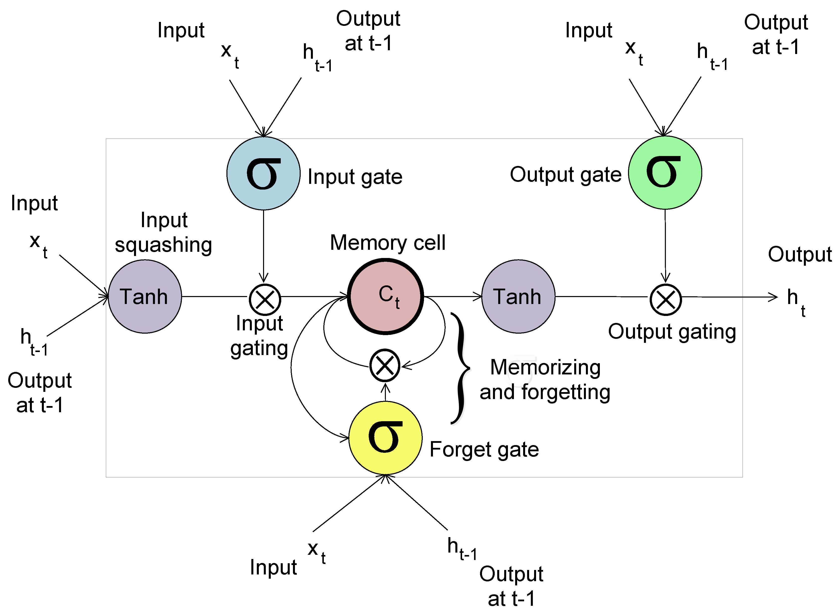
LSTM is a deep learning method that is a variant of RNN. It was first introduced by Hochreiter et al. in 1997 [43]. The basic purpose of proposing LSTM was to avoid the problem of vanishing gradient (using gradient descent algorithm), which occurs while training of back propagation neural network (as shown in Figure 1). The vanishing gradient leads to overfitting of the network on training data. The overfitting is the memorizing of inputs and not learning. An overfitted model is not generalized to perform well on unseen or test data. In LSTM, every neuron of the hidden layer is a memory cell, which contains a self-connected recurrent edge. This edge has a weight of 1, which makes the gradient pass across may steps without exploding or vanishing. The structure of on LSTM unit is shown in Figure 2.
LSTM consists of five basic units: memory block, memory cells, input gate, output gate and forget gate. All three gates are multiplicative and adaptive. These gates are shared with all the cells in the block. The memory cells have recurrent self-connected linear units known as Constant Error Carousel (CEC). The error and activation signals are recirculated by CEC, which makes it act as a short-term storage unit. The input, output and forget gates are trained to decide which information should be stored in memory, for what time period and when to read the information. The flow of a new input into the cell is controlled by input cell. The output cell decides: (i) the time extension for value in the cell to be used in output activation of LSTM unit and the forget gate; (ii) the memorizing period of memory cell’s value; and (iii) the forgetting time of the memory cell’s value. LSTM updates all the units in the time steps t = 0 , 1 , 2 , n , and compute the error signals for all the weights. The operation of units is referred to as the forward pass and error signal computation is known as a backward pass.

4.3.1. Forward Pass

The equations below represent the forward pass operations of the LSTM. j denotes the memory blocks. v is used for memory cells in a block j (that contains S j cells). c j v is the vth cell of the jth memory block. w l m is the connection weight between units m and l. The value of m ranges over all the source units. When the activation of source unit y m ( t 1 ) is referring to the input unit, the recent external input y m ( t ) is used. The calculation of y c output of c memory cell is based on the state of recent cell s c as well as the four sources of input: cell’s itself input z c , input gate’s input z in , forget gate’s input z φ and output gate’s input z out .
Input: The net cell input is calculated for every forward pass as follows:
z c j v ( t ) = m w c j v m y m ( t 1 )
After calculating the net input, the input squashing or transformation function g is applied to it.
Sigmoid function f in is applied to calculate the value of memory block input gate’s activation. f in is applied on the input of gate z in :
y in j ( t ) = f in j ( z in j ( t ) )
z in j ( t ) = m w in j m y m ( t 1 ) .
A product of z in and z c j v ( t ) is calculated. The input gate’s activation value y in is multiplied by all of the cells in the memory block to determine the activity patterns to be stored into memory. In training process, input gate learns to store the significant information in the memory block, by opening ( y in 1 ). It also learns to block out the irrelevant inputs by closing ( y in 0 ).
Cell State: Initially, the activation or state s c of a memory cell c is set to zero. During training, the CEC accumulates a sum of values, left by the forget gate. Memory block’s forget gate activation is calculated as:
y φ j ( t ) = f φ j ( z φ j ( t ) )
z φ j ( t ) = m w φ j m y m ( t 1 )
where f φ denotes the logistic sigmoid function of range [ 0 , 1 ] . The new cell state is calculated by addition of gated cell’s input with the product of forget gate activation and previous state:
s c j v ( t ) = y φ j ( t ) s c j v ( t 1 ) + y in j ( t ) g ( z c j v ( t ) ) , s c j v ( 0 ) = 0 .
While the forget gate is open ( y φ 1 ), the value keeps circulating in the CEC unit. When the input gate is learning to store in the memory, the forget gate is also learning the time duration of restraining an information. Once the information is outdated, the forget gate erases it and resets the memory cell’s state to zero, thus preventing the cell state to approach infinity and enabling it to store the fresh data without the interference of previous operations.
Output: The output of cell y c is calculated multiplying the cell state s c with the activation y out of the output gate of a memory cell:
y c j v ( t ) = y out j ( t ) s c j v ( t ) .
The forward pass operations of the LSTM are explained with the help of the aforementioned equations. The backward pass is explained in the next section.

4.3.2. Backward Pass

The objective function E is minimized by gradient descent function and weights w l m are updated. The weights are updated by an amount Δ w l m given by the learning rate α times the negative gradient of E. The weights of the output unit are updated by the standard back-propagation method:
Δ w k m ( t ) = α δ k ( t ) y m ( t 1 )
δ k ( t ) = E ( t ) z k ( t )
Based on the targets t k , squared error objective function is used:
δ k ( t ) = f k ( z k ( t ) ) e k ( t ) ,
where e k ( t ) = t k ( t ) y k ( t ) is the externally injected error. The weight changes for connections to the output gate (of the jth memory block) from source units m are also obtained by standard back-propagation:
Δ w out j m ( t ) = α δ out j ( t ) y m ( t )
The internal state error is represented by e s c j v . It is calculated for every memory cell:
e s c j v ( t ) = y out j ( t ) k w k c j v δ k ( t ) .
The aforementioned equations describe the forward pass, backward pass and learning process of a single LSTM unit. Several LSTM units are connected together in a series to form the LSTM network. The output of one unit becomes the input of the next unit.

4.3.3. Deep LSTM

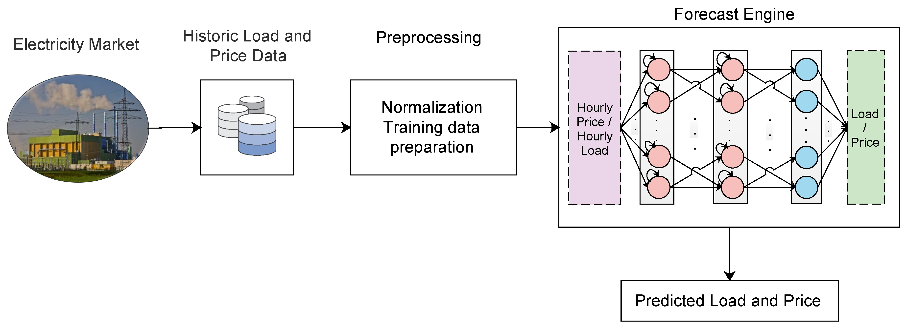
The functionality of traditional LSTM is explained in the previous section. In this section, the working of the proposed algorithm DLSTM is discussed in detail. The proposed method comprises of four main parts: preprocessing of data, training LSTM network, validation of network, forecasting load and price on test data. The system model is shown in Figure 3.
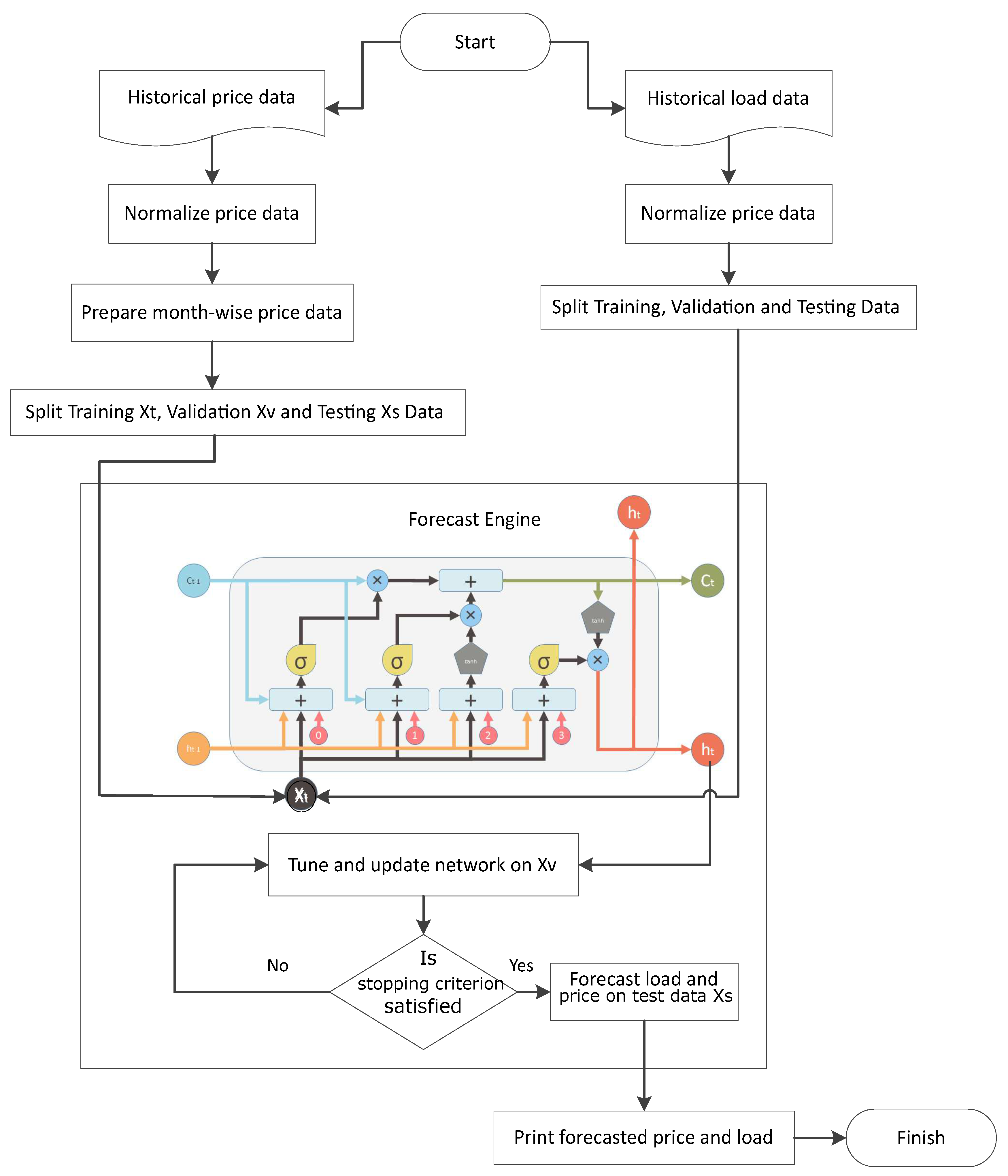
The steps in the proposed model are listed as follows:
  • Step 1: The historical price and load vectors are p and l, respectively, which are normalized as:
    p n o r = p m e a n ( p ) s t d ( p )
    where p n o r is vector of normalized price, m e a n ( ) is the function to calculate average and s t d ( ) is the function to calculate standard deviation. This normalization is known as zero mean unit variance normalization. Price data are split month-wise. Data are divided into three partitions: train, validate and test.
  • Step 2: Network is trained on training data and tested on validation data. NRMSE is calculated on validation data.
  • Step 3: Network is tuned and updated on actual values of validation data.
  • Step 4: The upgraded network is tested on the test data where day ahead, week ahead and month ahead prices and load are forecasted. Forecaster’s performance is evaluated by calculating the NRMSE.
The step-by-step flowchart of the proposed method is shown in Figure 4.

4.4. Data Preprocessing

Hourly data of regulation market capacity clearing price and system load were acquired from ISO NE and NYISO. The data of ISO NE represent eight years, i.e., from January 2011 to March 2018. Data comprise price and load of seven complete years, i.e., 2011 to 2017. Only three months of data are available for 2018, i.e., January to March. The data of NYISO (New York City) represent 13 years, i.e., January 2006 to September 2018. The NYISO data comprise 12 complete years, i.e., 2006 to 2017. For 2018, nine months of data were acquired, i.e., January to September. The data were divided month-wise. For example, data of January 2011, January 2012, , January 2018 were combined, all twelve months data were combined in the same fashion. The DLSTM network was trained on month-wise data. Data were partitioned into three parts: train, validation and test data.

4.5. Network Training and Forecasting

Training, validation and test data were obtained by preprocessing the data. The price and load data were fed to the DLSTM network for training.
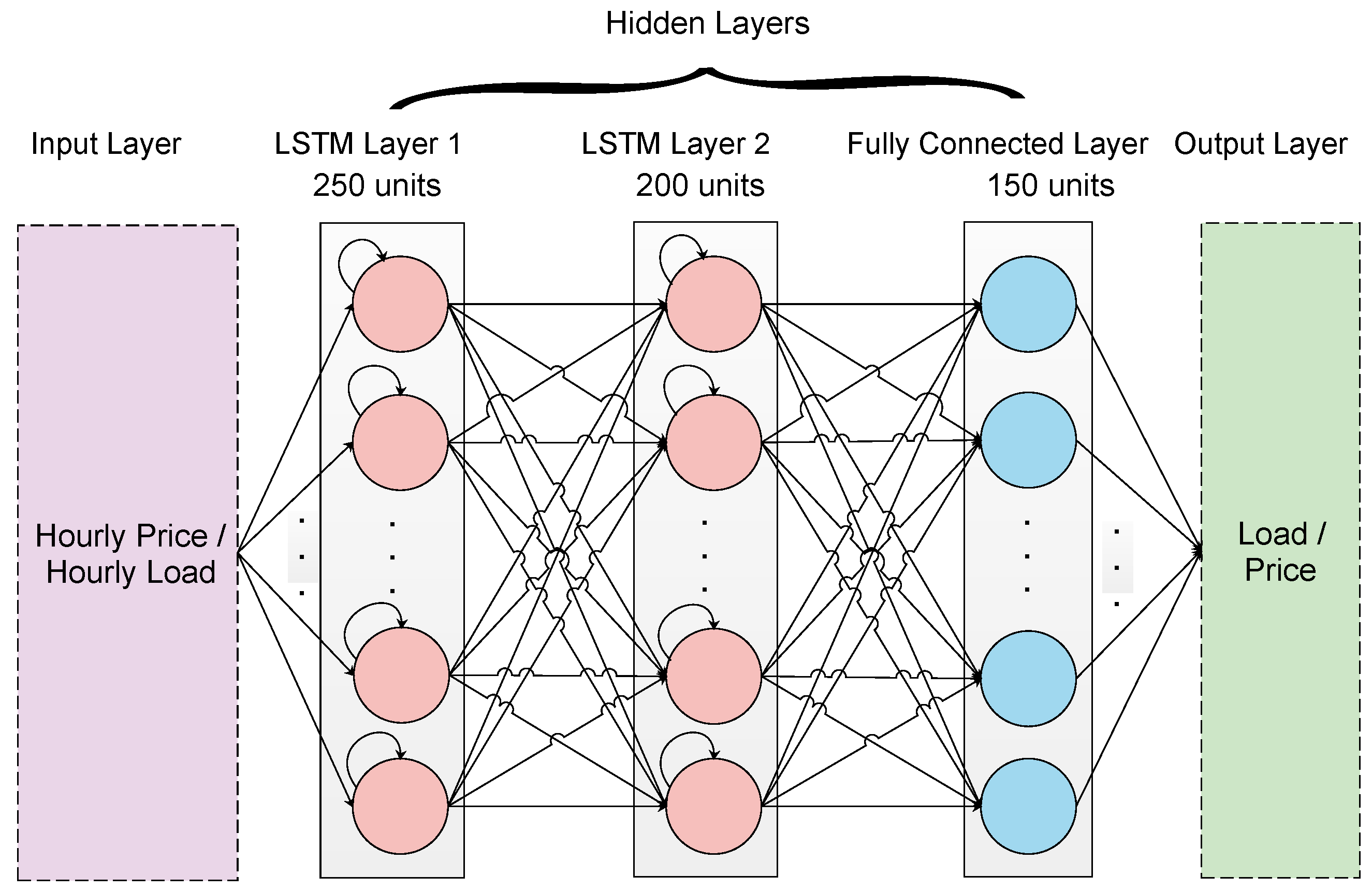
The proposed DLSTM has five layers, i.e., an input layer, two LSTM layers, a fully connected layer and the regression output layer. The number of hidden units in LSTM layer 1 is 250, and LSTM layer 2 is 200. The final number of hidden units were decided after experimenting on a different number of hidden units and keeping the number of hidden units with the least forecast error. During the training process of DLSTM, the network predicts step ahead values at every time step. The DLSTM learns patterns of data at every time step and updates the network trained until the previous time step. Every predicted value is made part of the whole data for the next prediction. In this manner, the network is adaptively trained. DLSTM network is trained for price and load data separately. The network trained on training data is the initial network. Initial network is tested on validation data. The initial network forecasts step ahead value on validation data. After taking forecast results from the initial network, the NRMSE is calculated. The initial network re-learns and re-tunes on actual values of validation data until the NRMSE reduces to a minimum. Now, the final and tuned network is used to forecast price and load. The architecture of the proposed forecast method is shown in Figure 5.

4.6. Implementation Details

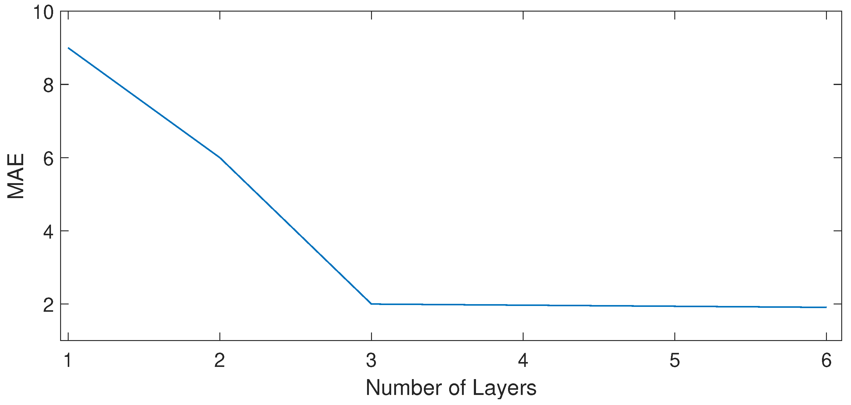
The number of network layers and neurons in every layer affect the prediction accuracy. The number of layers and the hidden units was finalized after several experiments. Increasing number of layers increases the computational complexity and time. Layers were added one by one and accuracy was measured. There was no significant increase in forecasting accuracy after adding three hidden layers, as shown in Figure 6. The hidden layer is the LSTM layer, the second hidden layer is also an LSTM layer and the third hidden layer is a fully connected layer with 250, 200 and 150 hidden units, respectively. The output layer is a regression layer. All remaining parameters of the network were finalized according to best accuracy. The learning rate was set to 0.001. Adam (Adaptive Moment Estimation) optimizer algorithm is used for adaptive optimization of weights during training. Initial momentum was set to be 0.9. The maximum number of epochs was set to be 250. The training of network was stopped if the learning error stopped decreasing significantly or maximum epoch was reached.

4.7. Network Stability

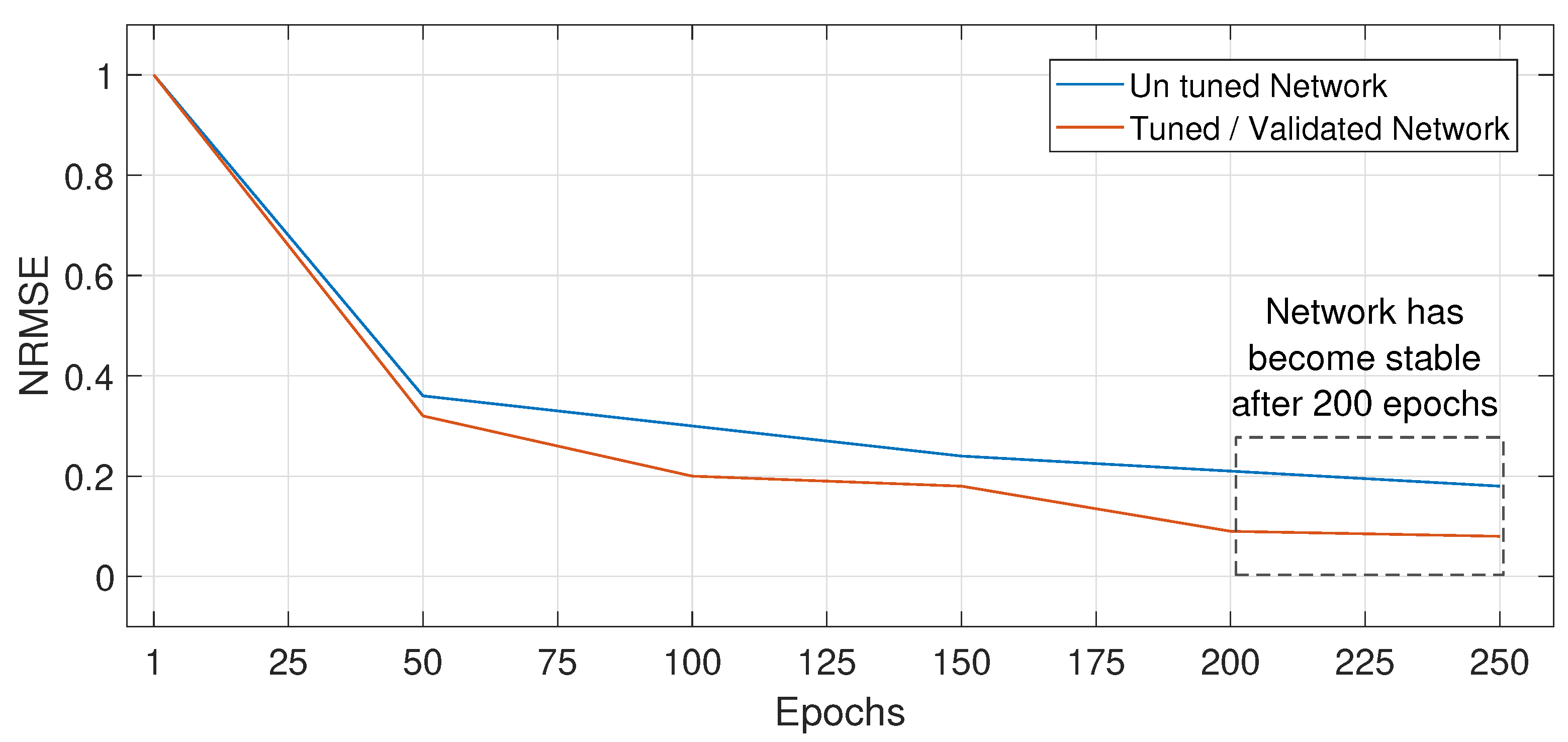
A neural network becomes stable when the training or testing error stops reducing after a certain value. At this point, the weights are optimized and changes in weights are very small, therefore the error reduction becomes negligible [45]. The learned and finely tuned weights produce accurate forecast result. The complete data are leaned and the pattern of data are extracted well when the network becomes stable. To achieve stability quickly, the inputs, learning rate, momentum, etc. can be changed. The stability of the proposed network was achieved after 200 epochs, where the NRMSE reduced to 0.08 (Figure 7). In Figure 7, the stability of the network is highlighted in a rectangle, where the error drop almost becomes zero, showing a straight line. The error drop and epochs are shown for both the networks: initial and fine-tuned after validation. Both networks converge or become stable after the 200 epochs. It is clear that the minimum error of the initial un-tuned network is higher as compared to the validated network. It verifies that the validation is beneficial in improving the accuracy of the network.

5. Results and Discussion

This section covers the experimental results of the proposed forecast method. In this section, the qualitative and quantitative analysis are given for the proposed forecast method. The graphical analyses of data and prediction results are presented in Figure 8, Figure 9, Figure 10, Figure 11, Figure 12, Figure 13, Figure 14, Figure 15, Figure 16, Figure 17, Figure 18, Figure 19, Figure 20, Figure 21, Figure 22, Figure 23, Figure 24, Figure 25, Figure 26, Figure 27 and Figure 28.

5.1. Working of DLSTM

The DLSTM network works on the train and update state method. At a time step, the networks learns a value of price or load time series and stores a state. On the next time step, the network learns the next value and updates the state of previously learned network. All data are learned in the same fashion to train the network. While testing, the last value of training data is taken as the initial input. One value is predicted at a time step. Now, this predicted value is made the part of training data and network is trained and updated. Every predicted value is made the part of the training data to predict the next value. For example, if network d l s t m n is learned on n values, the nth value is the input to predict the n + 1 th value. After predicting the n + 1 th value, the network d l s t m n + 1 is now trained and updated on n + 1 values to predict the n + 2 th value. The n + 1 th value is the first predicted value by the initially learned network d l s t m n . To predict m values, the network will train and update m times. After predicting m values, the last trained and updated network d l s t m n + m is trained on n + m values, i.e., n , n + 1 , n + 2 , n + m 1 .

5.2. Data Description

The historic electricity price and load data used in simulations were taken from ISO NE [41] and NYISO [42]. ISO NE manages the generation and transmission system of New England. ISO NE produces and transmits almost 30,000 MW electric energy daily. In ISO NE, annually 10 million dollars of transactions are completed by 400 electricity market participants. The data comprise ISO NE control area’s hourly system load and regulation capacity clearing price of 21 states of the USA captured in the last eight years, i.e., January 2011 to March 2018. The data contain 63,528 measurements.
NYISO is a not-for-profit corporation that operates New York’s bulk electricity grid and administers the state’s wholesale electricity markets. The data taken from NYISO are hourly consumption and price of New York City. The duration of data is thirteen years, i.e., January 2006 to October 2018. Total measurements are 112,300.
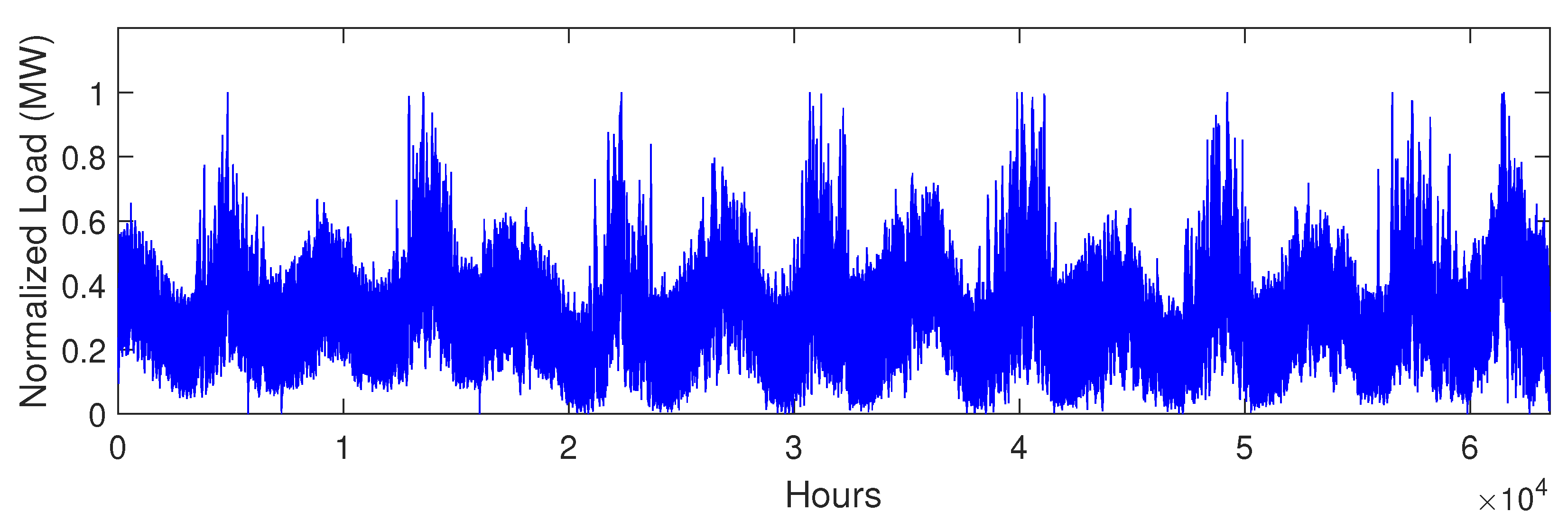
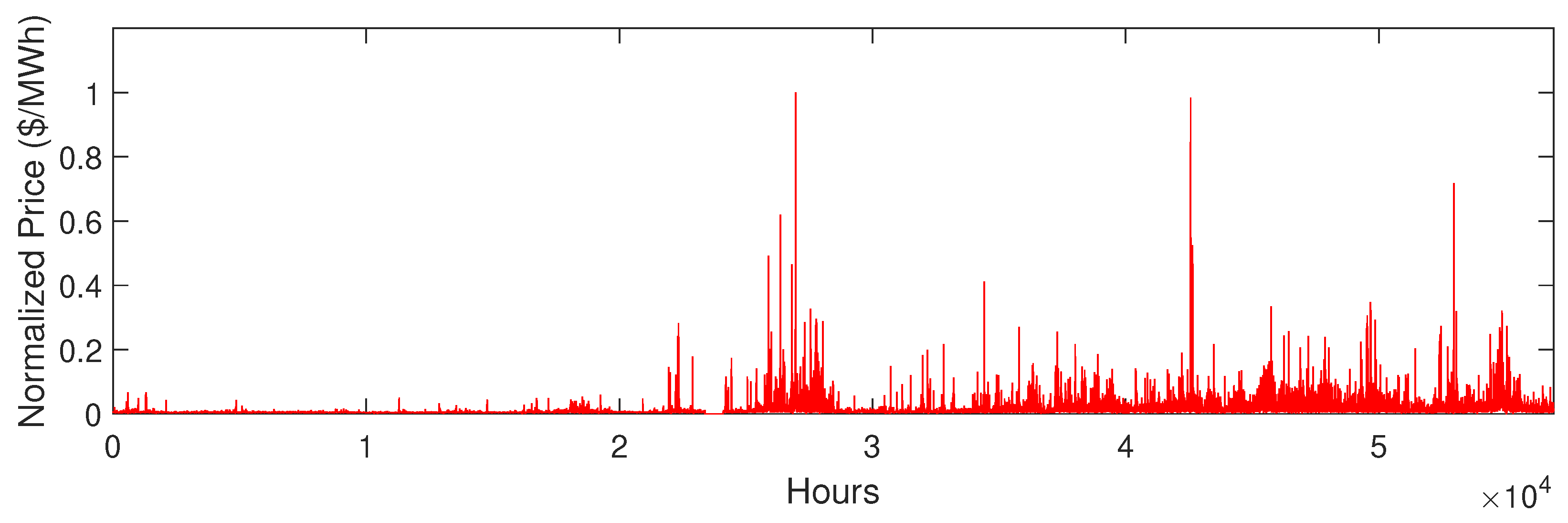
The electricity prices and load are significantly affected by seasonality. In proposed work, inter-season prices and load variations are also handled. Data were split month-wise, which improves the forecast accuracy. Inter-season splitting of data helps in efficient capturing of the highly varying price trend. The electricity load exhibits a repetitive pattern over the years. On the other hand, price pattern changes very drastically and stochastically. Both load and price increase over the years. It is clearly shown in Figure 8 that load increase with a constant rate and trend of load profile remains the same, whereas the price is increasing without any pattern similar to the one observed in the load profile. Price signals have a wide range of values sudden increase in spikes. The extremely volatile nature of energy price makes forecasting of price very difficult. The price trend is too random to handle by any forecasting algorithm. The price pattern is shown in Figure 9. The repetitive pattern of the load is caused by the same consumption times; the consumption hours always remain the same. There is more consumption in working hours and less in off hours and late night. There are several reasons behind the price’s varying patterns: (1) the amount of generation, which is inversely proportional to electricity price; (2) the source of electricity generation, which increases the price if fuel is used for generation and reduces the price if renewable resources are used for generation; (3) the price of fuel used for power generation; (4) government increments in price or taxes; and (5) excessive use of electricity penalty.
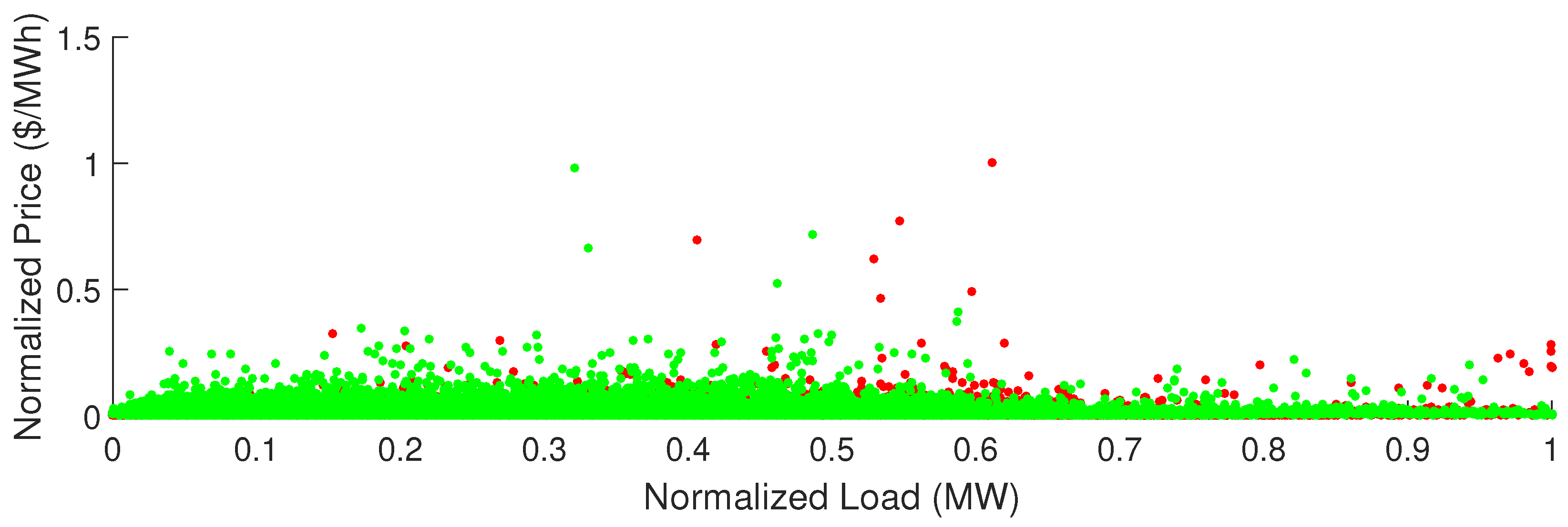
Electricity price and load are directly proportional. The relationship between electricity load and price is shown in Figure 10. It is clearly shown in the figures that price increases with increase in load in most cases. However, there are a few exceptional cases, where price is much higher than load.
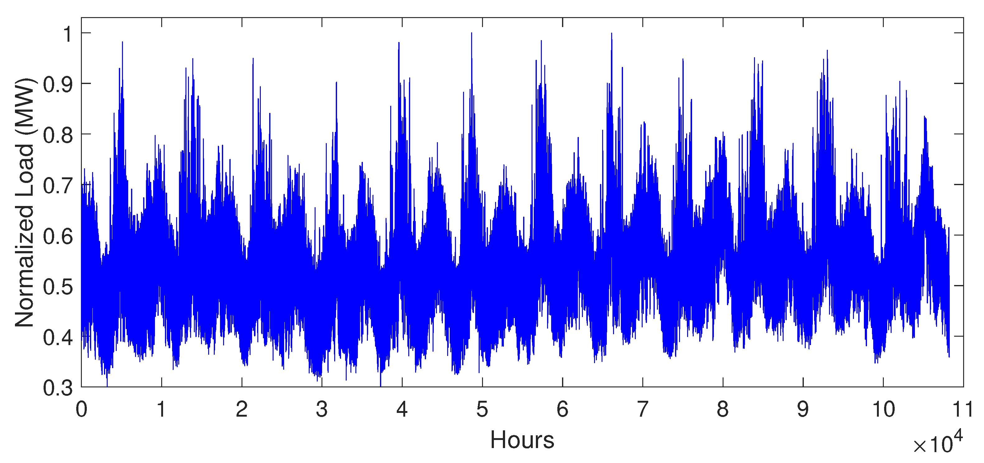
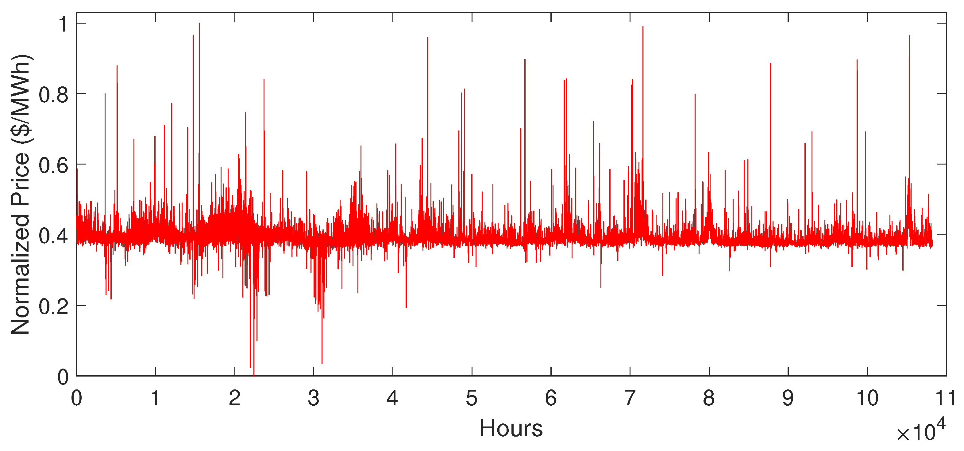
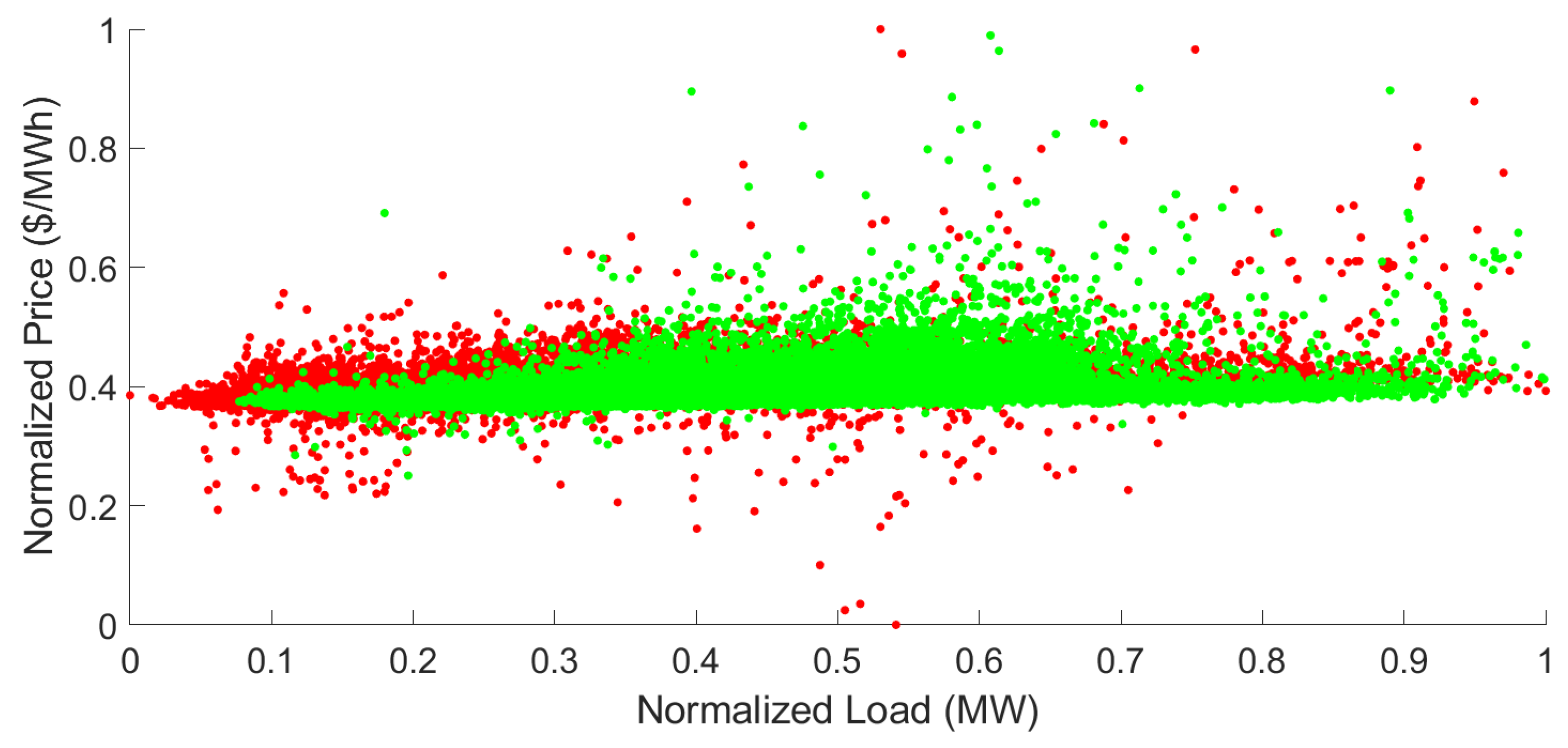
The trends of NYISO data are presented in Figure 11, Figure 12 and Figure 13.

5.3. Simulation Results

All simulation were performed using MATLAB R2018a on a computer system having core i3 processor. Two cases were studied. The first case was short-term forecasting (one day and one week) using aggregated load and the average price of six states. In the second case short- and medium-term (one month) load and price were forecasted using the data of one city, i.e., New York City. In this section, both case studies are discussed in detail.

5.3.1. Case Study 1

First, load data were taken to train forecast model. After normalization, the load profile trend showed a monotonous pattern (Figure 8). The load data were given for network training after normalization. The network was trained on 325 weeks, validated on 50 weeks and tested for 1 week. Without validation, the forecast results were worse. The DLSTM forecast result is a flat trend without the validation of the network. The network tuned and updated its previous state on real values of validation data.
The hourly system load from 1 January 2011 to 31 March 2018 is shown in Figure 8. Electricity load shows a similar pattern over the years. The hourly price from 1 January 2011 to 31 March 2018 is shown in Figure 9, which depicts the electricity price has a stochastic nature with sharp price spikes and it increases continuously. Figure 10 shows the relation between load and price signals from 1 February 2018 to 31 March 2018. An eight-year dataset was considered. The dataset was divided into 12 parts for 12 months of a year.
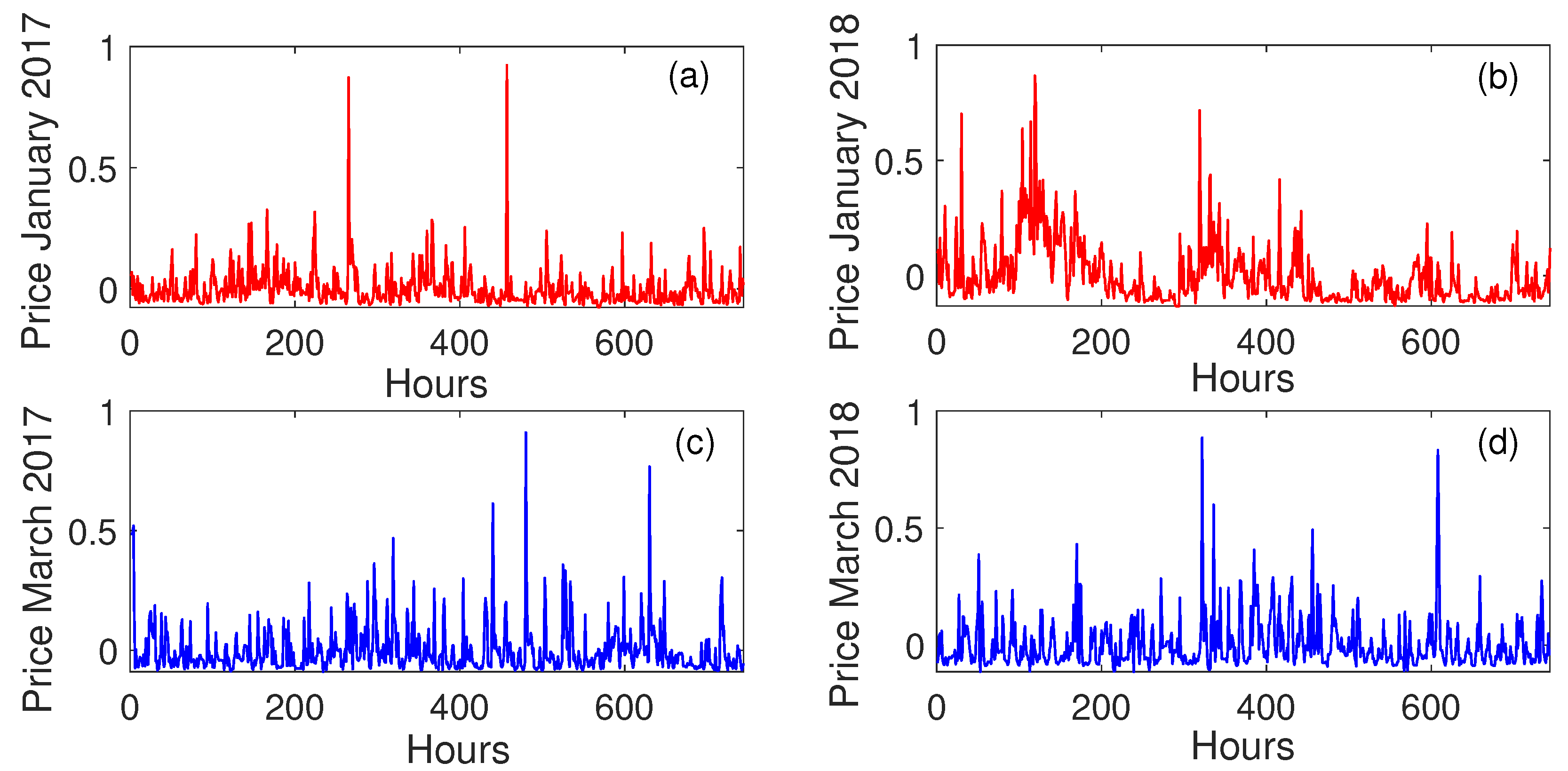
In Figure 14a, price signals of January 2017 are shown, whereas Figure 14b shows price signals of January 2018. Figure 14c illustrates the price signals of March 2017 and Figure 14d shows the price signals of March 2018. The price signals of same months, e.g., March 2017 and March 2018, show a similar pattern. The reason behind the similar price signals of same months of different years is the same weather conditions. In January 2018, there was an increase in the price between Hours 100 and 150 and Hours 200 and 300. Although the general patterns of the January 2017 and 2018 prices were the same, the increase in price in the aforementioned hours of January 2018 was higher than those of January 2017. This unexpected increase was due to the unavailability of cheaper electricity generation resources (i.e., photovoltaic generation and windmill generation). It is clear from the results in Figure 14 that the patterns of price signal of different months, e.g., January 2018 and March 2018 are different. Every year, the weather is colder in January and moderate in March. Due to the weather conditions, the heating and cooling loads are similar every year, which directly impact the price. Therefore, the forecast model was trained on data of January 2011, January 2012, , January 2018 (first three weeks) to forecast the price of the last week of January 2018. The month-wise splitting of input data helped improve the forecast accuracy. On the other hand, if input data were not split, the forecast accuracy degraded to an unacceptable level.
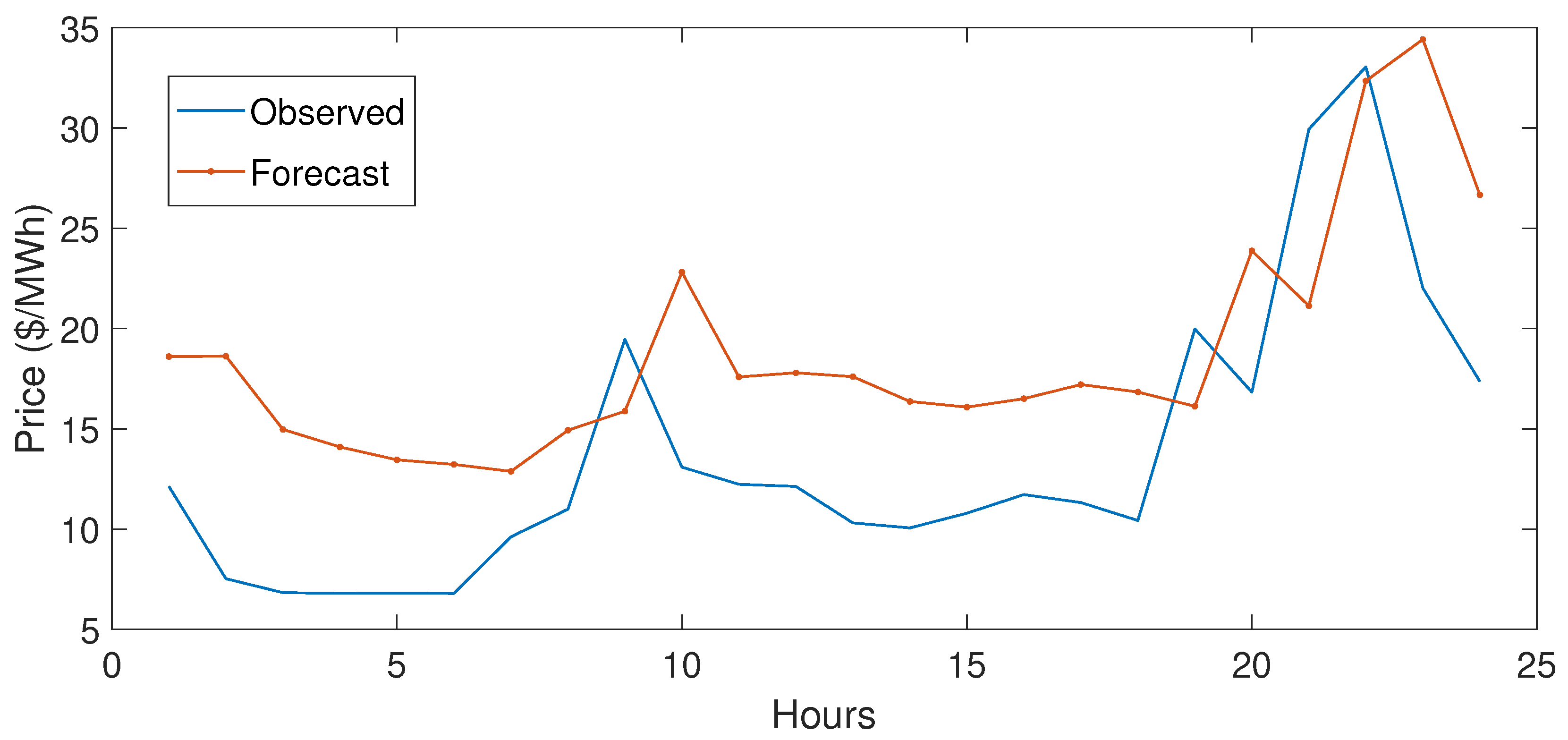
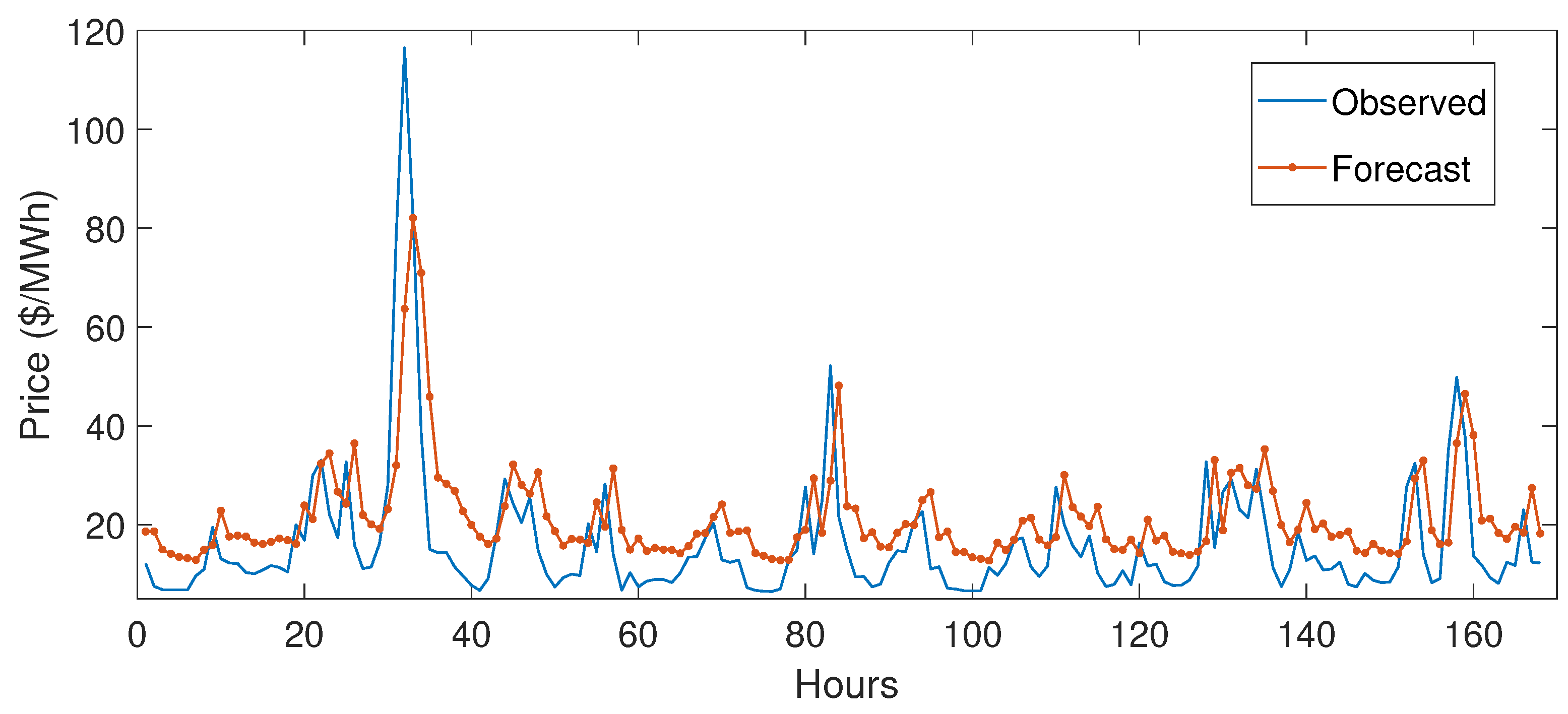
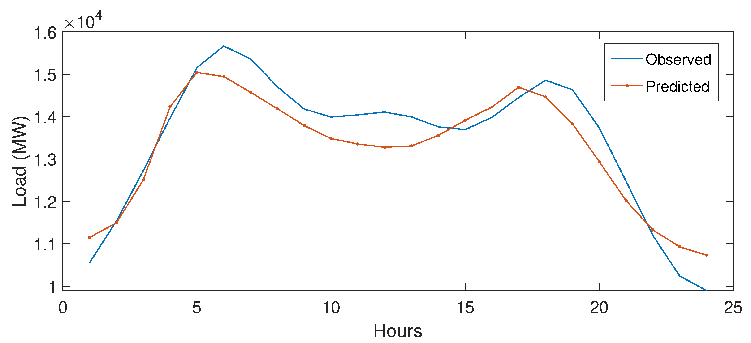
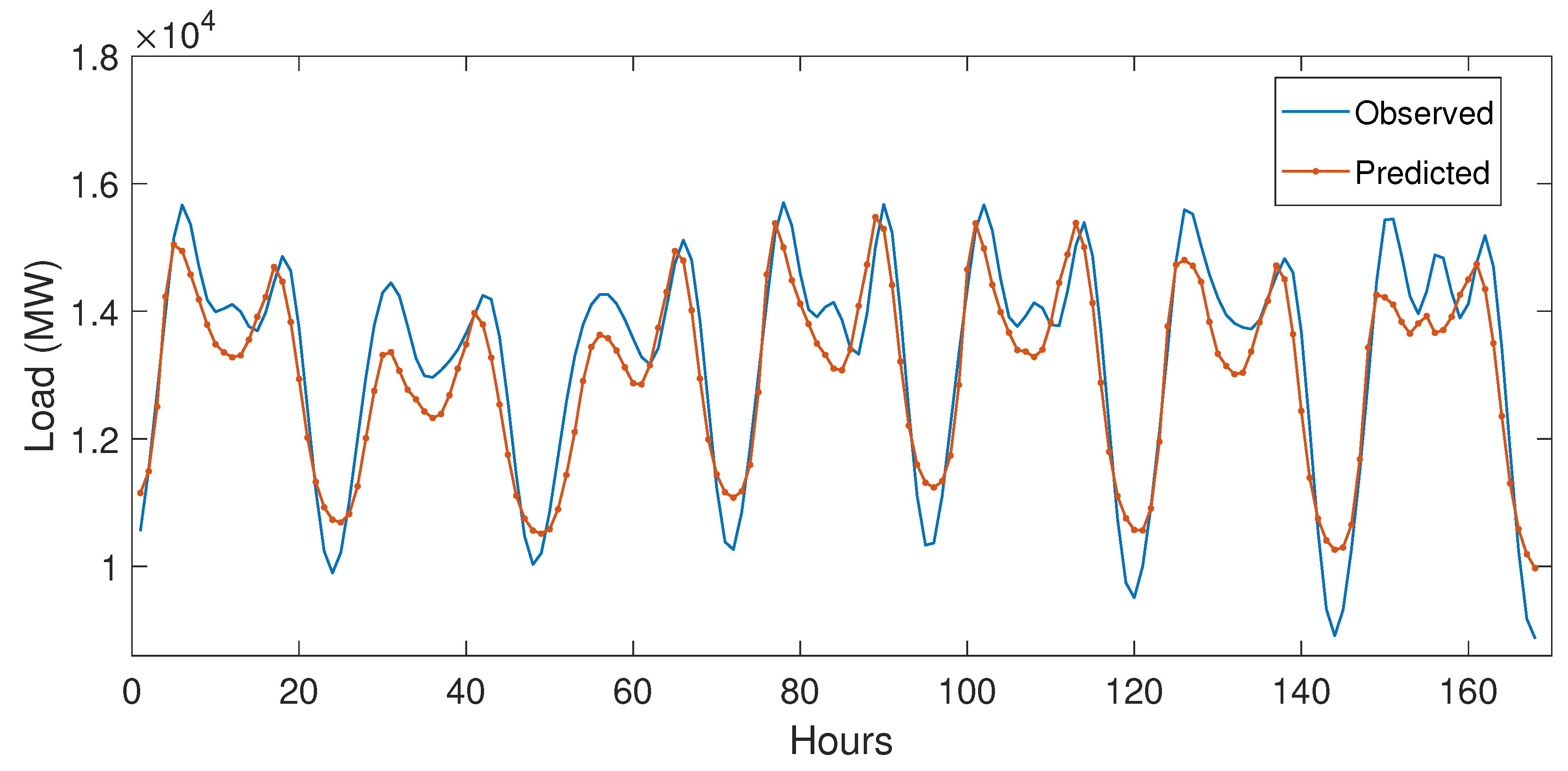
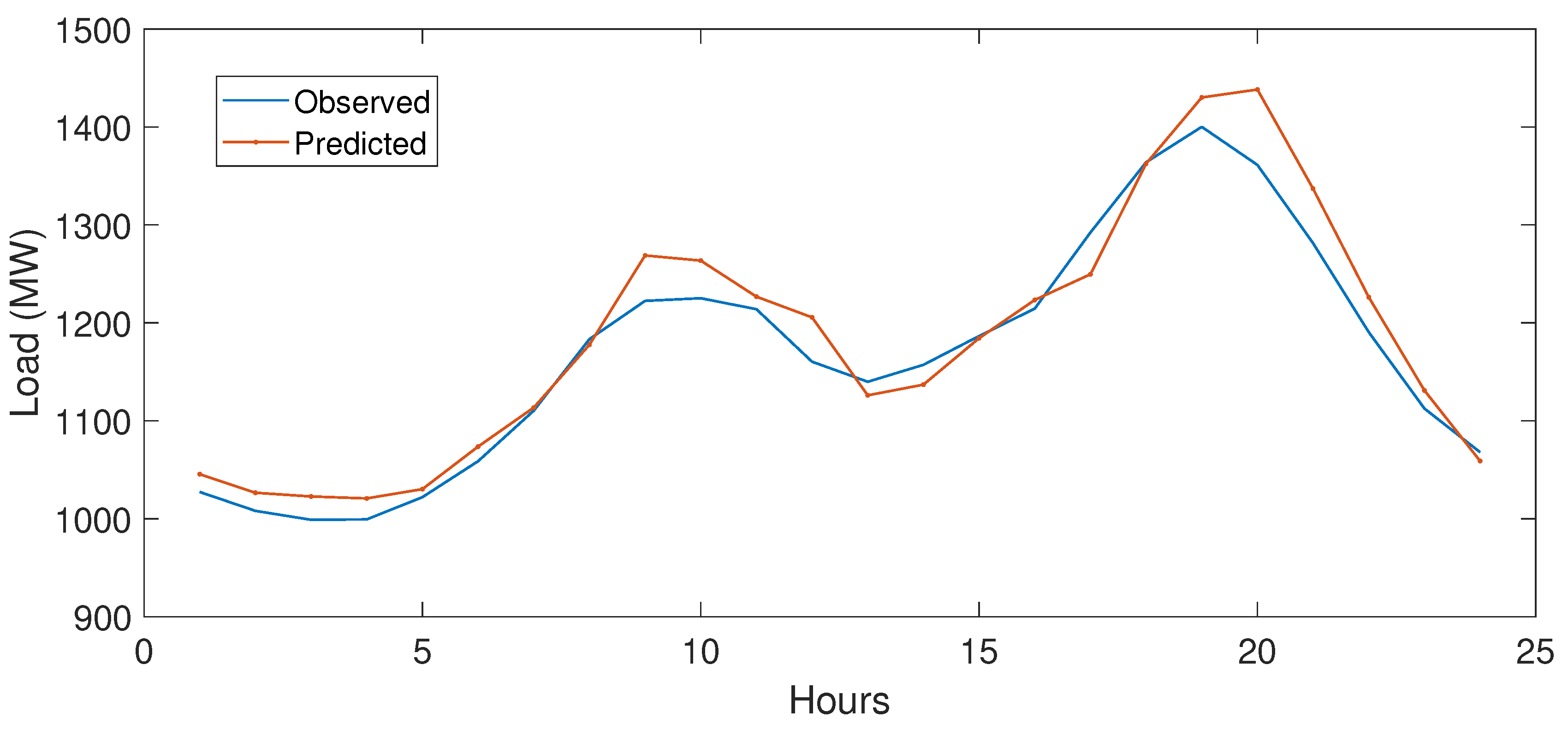
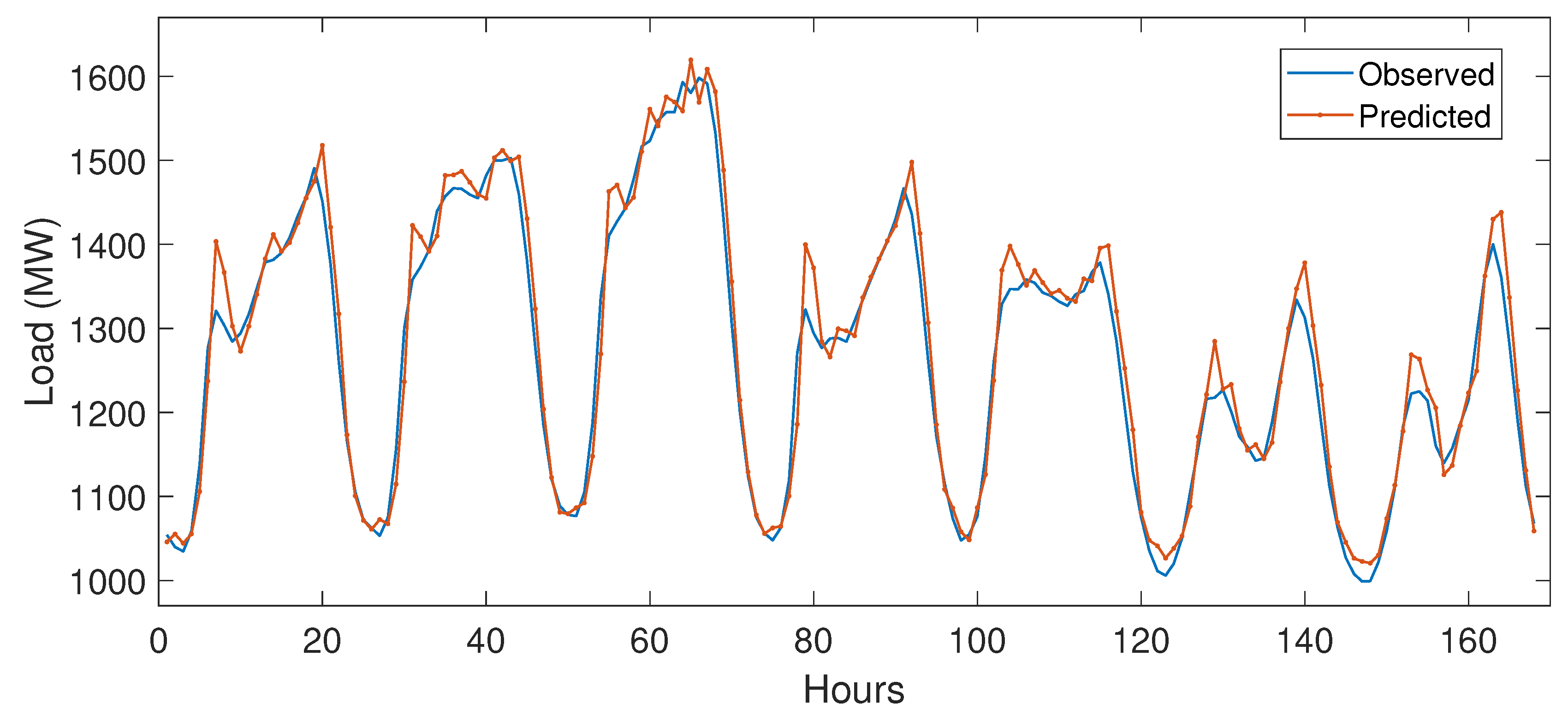
Figure 15 illustrates the actual and forecasted price of 23 March 2018. Figure 16 is the price forecast of last week of March 2018. Figure 17 and Figure 18 present the predicted load of one day and one weak.

5.3.2. Case Study 2

Thirteen years (i.e., January 2006 to March 2018) load and price data of New York City were used for medium-term forecasting. The normalized load is shown in Figure 11. The price signals of 13 years are shown in Figure 12. The relation of price and load signals of New York City is shown in the scatter plot of Figure 13.
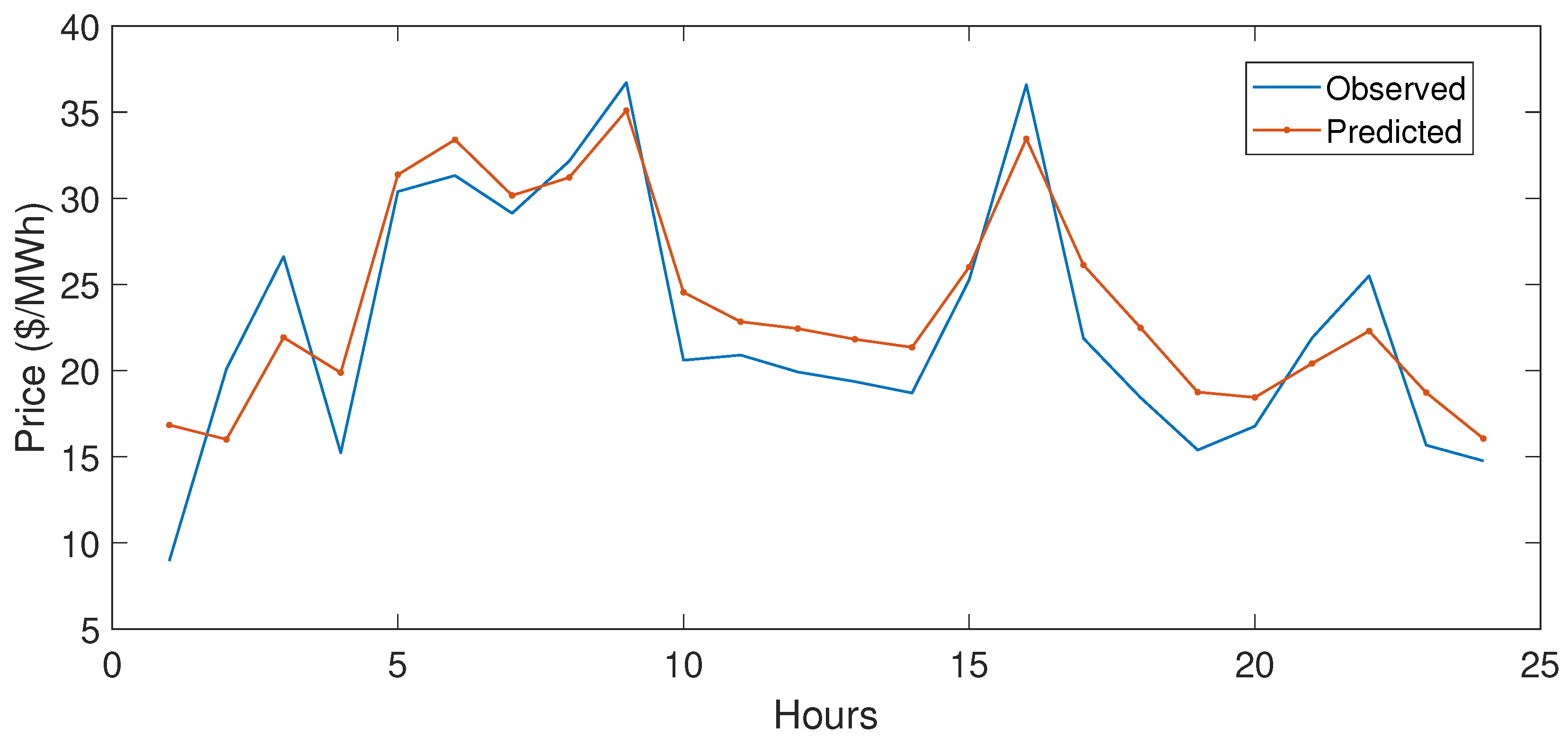
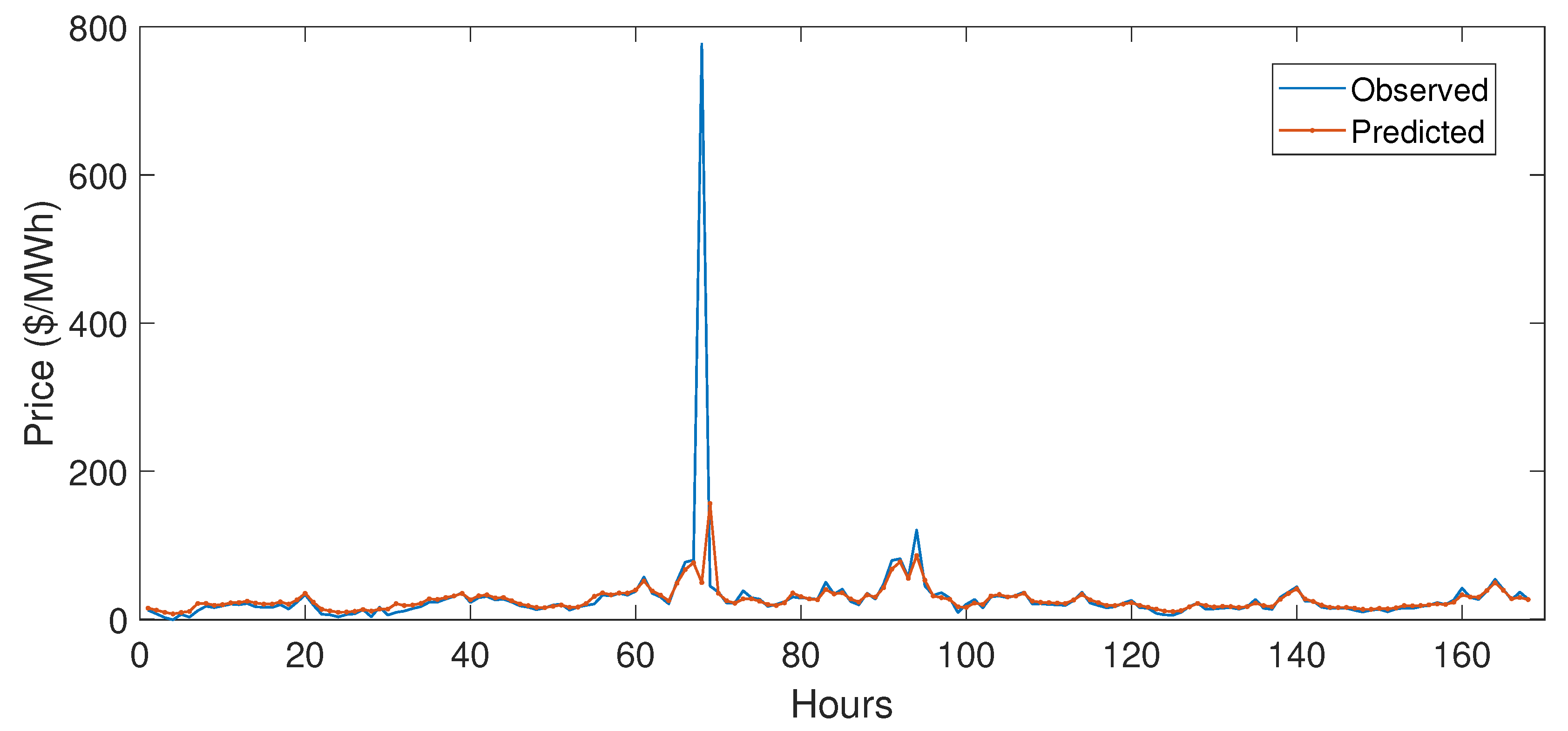
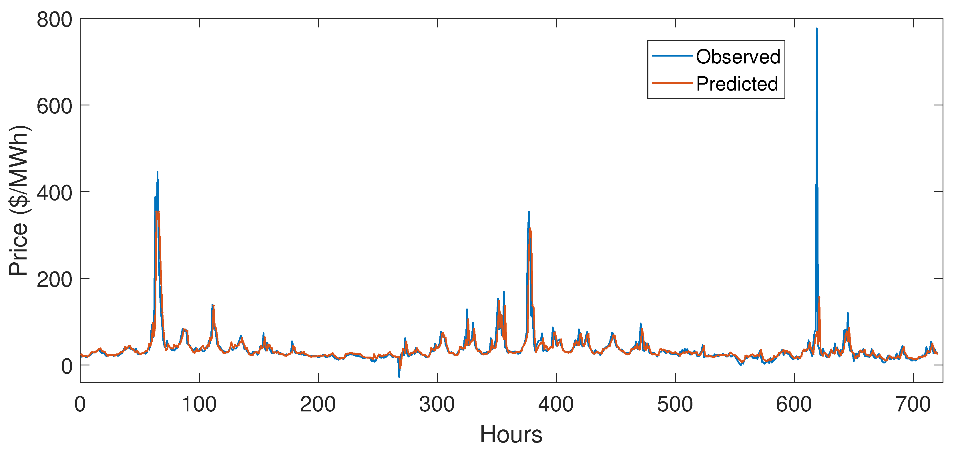
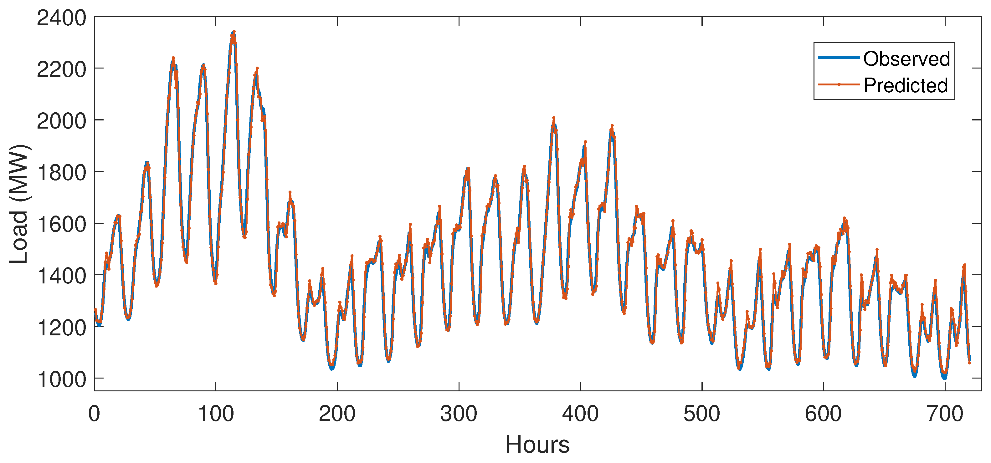
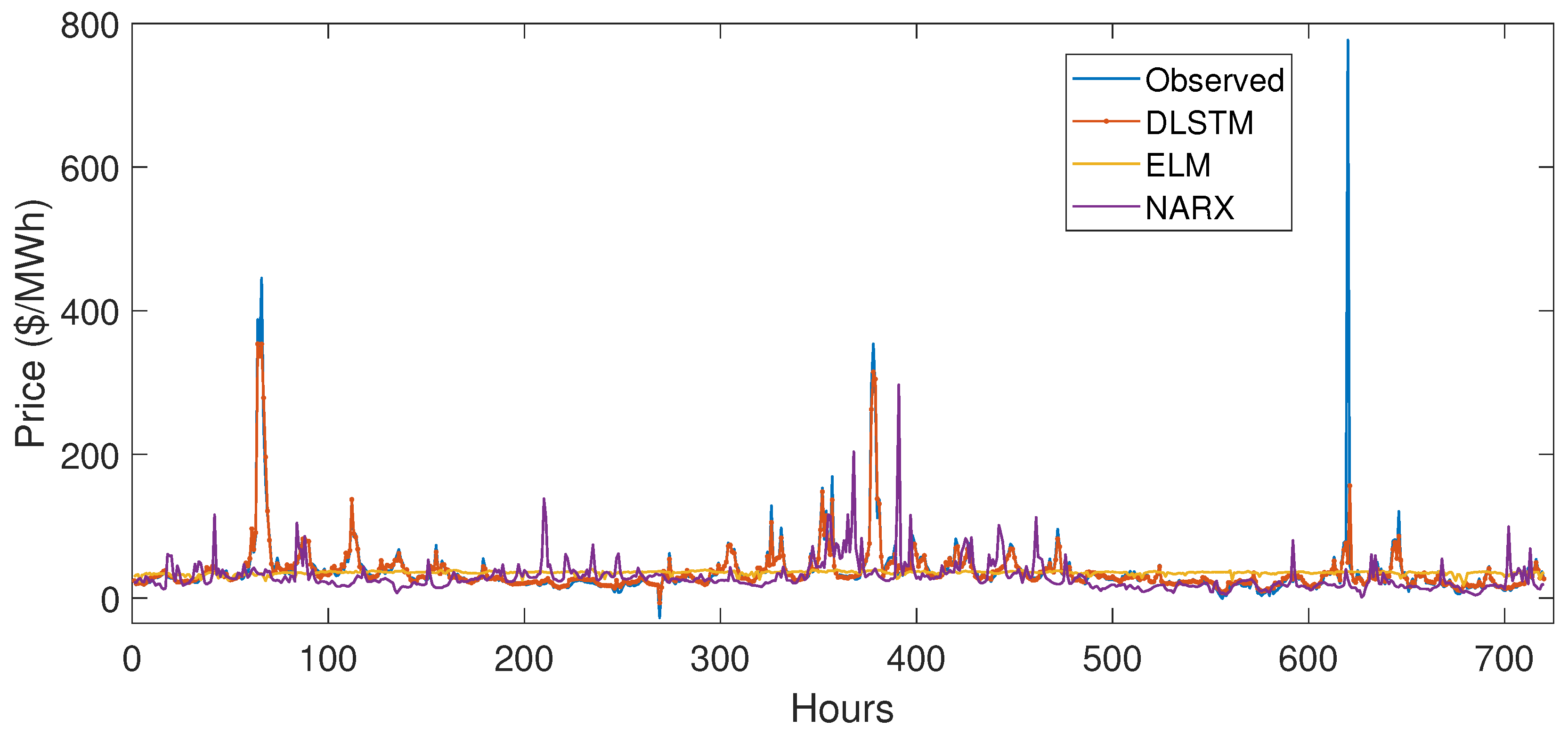
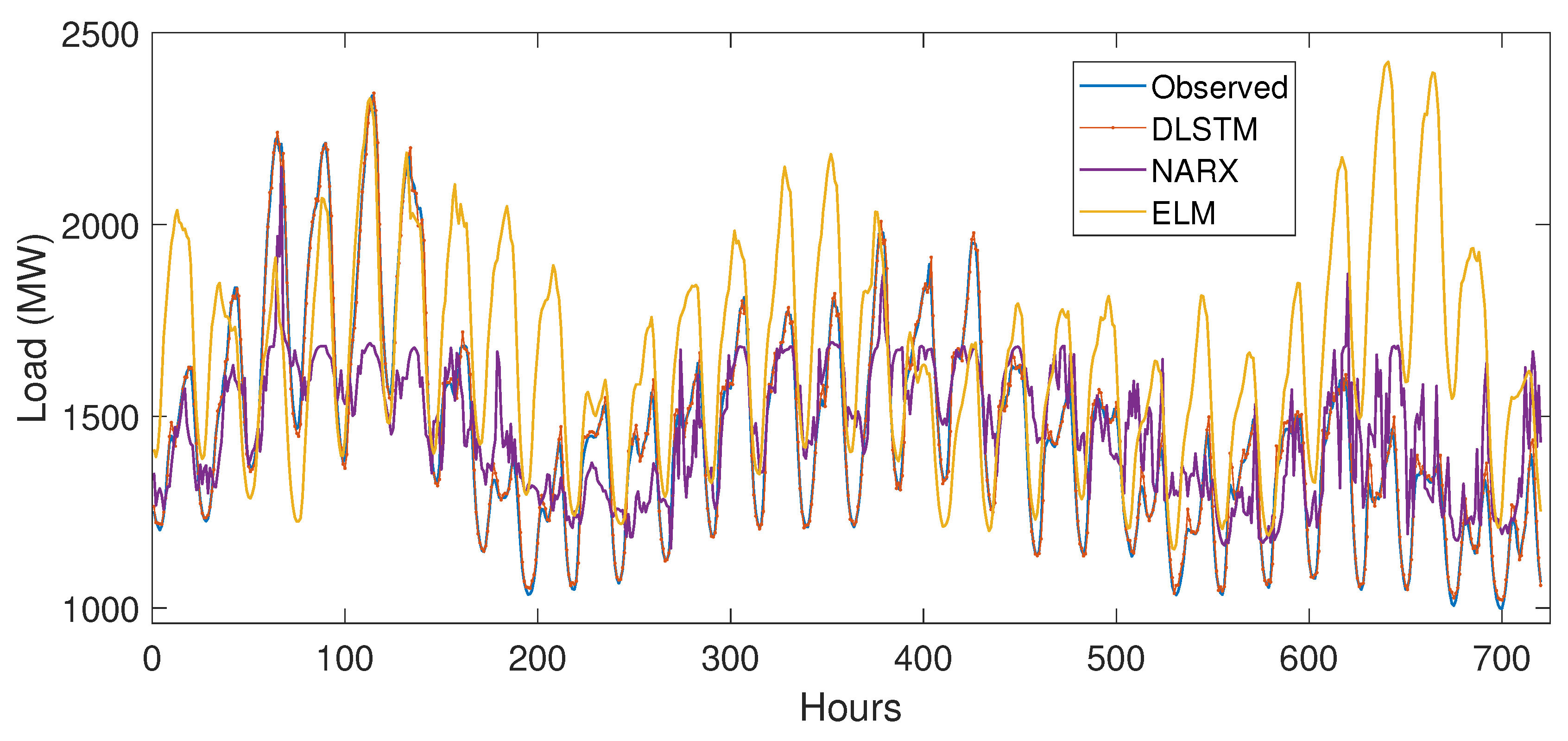
For medium-term forecasting, load and price of one month (September 2018) were forecasted, for a total of 720 h. Forecasting results of one day (24 h) and one week (168 h) are also shown. Price forecast of one day and one week are shown in Figure 19 and Figure 20, respectively. Forecasted price from 1 September 2018 to 30 September 2018 is shown in Figure 21. Load forecast of one day and one week are shown in Figure 22 and Figure 23, respectively. The 1 month forecasted load is shown in Figure 24. The load and price forecast of New York City were more accurate compared to the forecast on aggregated data of ISO NE. The ISO NE data comprise aggregated load and average price of six states. The reason for NYISO’s better accuracy is its larger size of data as compared to ISO NE. The total number of measurements in ISO NE are 63,528 and NYISO are 112,300. It is the characteristic of deep learning that its performance improves with the increase in the size of data [39].
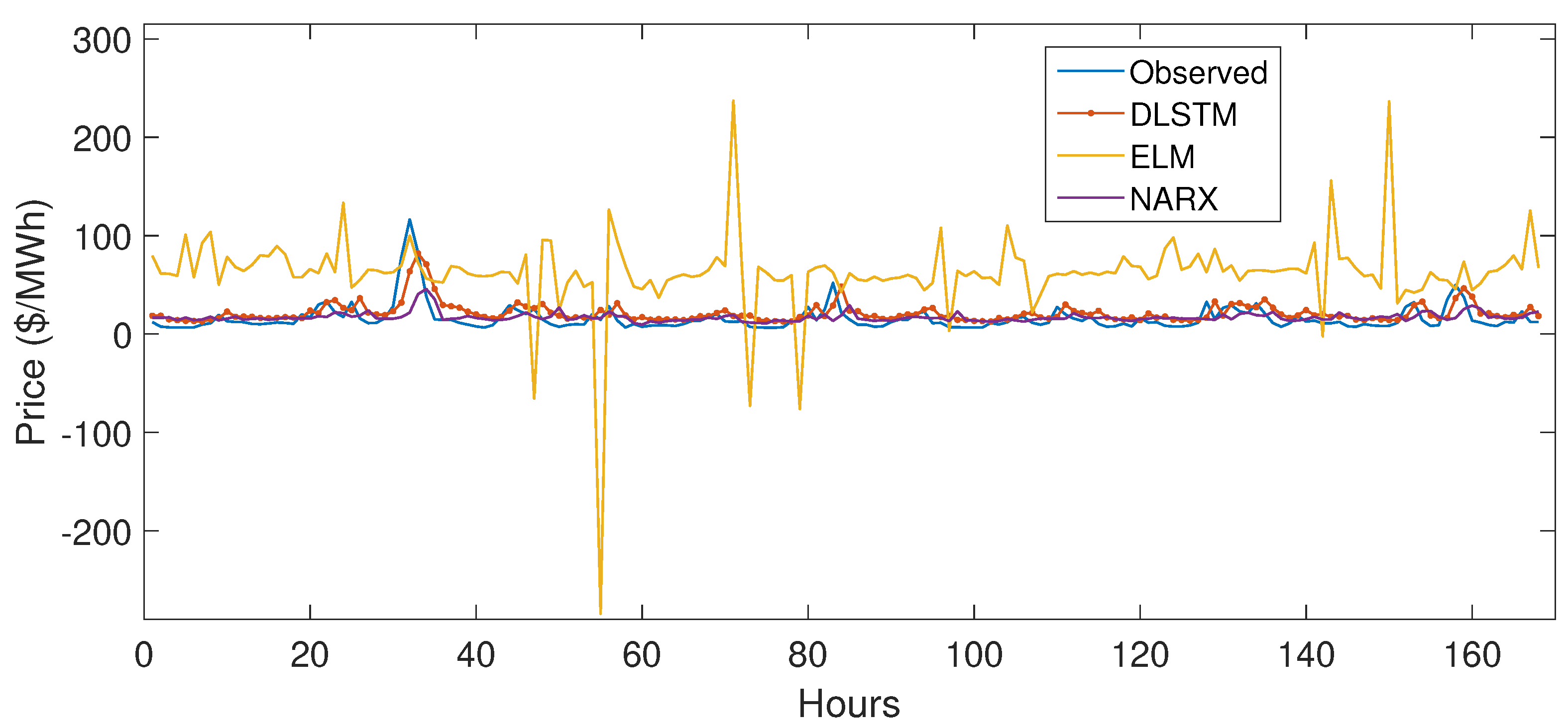
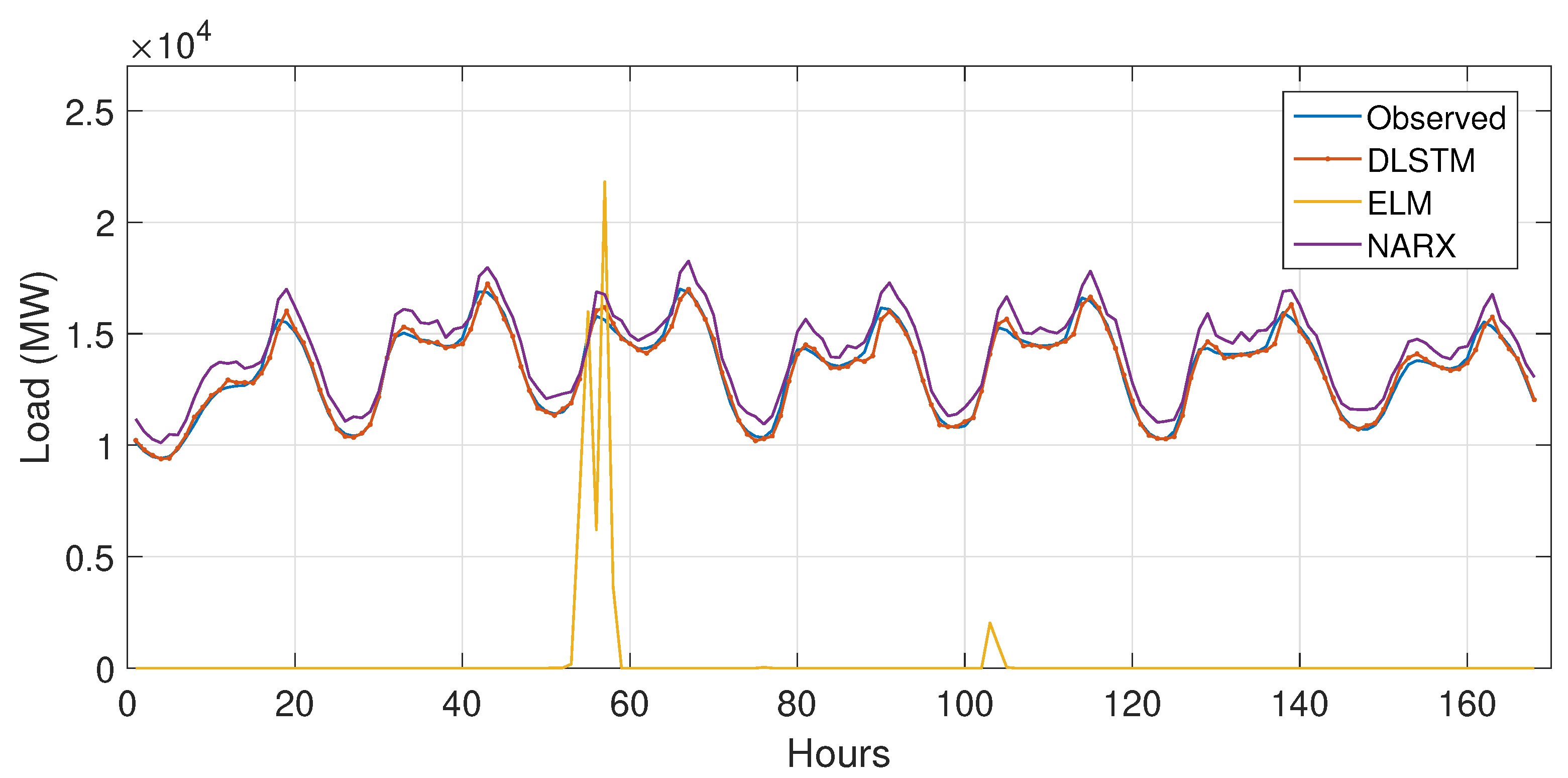
Figure 16 illustrates actual and forecasted price of last week of March 2018. Figure 25 illustrates the performance comparison of proposed deep LSTM with the well known time series forecasting methods for price forecasting. In Figure 26, comparison of DLSTM is shown for the load forecasting. The MAE and NRMSE are shown for the day ahead load and price forecast.
The performance of the proposed method was compared with well-known forecasting methods: ELM, Wavelet Transform (WT) + Self Adaptive Particle Swarm Optimization (SAPSO) + Kernel ELM (KELM) (WT + SAPSO + KELM) [46], NARX and Improved NARX (INARX) [47]. When the performance of DLSTM was compared with the aforementioned methods, it had less error. DLSTM had lower MAE and NRMSE as compared to ELM, WT+SAPSO+KELM, NARX and INARX. WT+SAPSO+KELM [46] is proposed for electricity price prediction. For price forecasting, DLSTM was compared with ELM, NARX and WT + SAPSO + KELM. Buitrago et al. proposed INARX [47] for electricity load prediction. The DLTM load prediction results were compared with ELM, NARX and INARX. The comparison of forecast results is shown in Figure 27 and Figure 28. DLSTM forecasted accurately compared to ELM, WT + SAPSO + KELM, NARX and INARX. ELM is a feed-forward ANN. Its weights are set once and never changed afterwards. For good performance of ELM, the weights should be optimized. ELM can only perform well if the weights are optimized, because its weights cannot change during the training of the network. NARX performed better as compared to ELM. Unlike ELM, NARX has a feed back architecture. It has a recurrent ANN like DLSTM. NARX performance is reasonable for load forecast (Figure 28), however it is unable to model the high seasonality and volatility of price signals (Figure 27). DLSTM has a feedback architecture, where errors are backpropagated. In DLSTM, weights are updated multiple times during training, with every new input. The learned weights are obtained when network completes its training on complete training data.

5.4. Performance Evaluation

For performance evaluation, two evaluation indicators were used: MAE and NRMSE. MAPE performance matric has a limitation of being infinite, if the denominator is zero; MAPE is negative, if the values are negative, which are considered meaningless. Therefore, MAE and NRMSE are suitable performance measures. The formulas of MAE and NRMSE are given in Equations (18) and (19), respectively.
M A E = 1 T t = 1 T | ( X s y s ) |
N R M S E = 1 T t = 1 T ( X s y s ) 2 ( m a x ( X s ) m i n ( X s ) )
where X s is the observed test value at time t and y s is forecasted value at time t.
The last week of every month was tested; starting from May 2017 to April 2018. Twelve weeks were tested. The performance of every month is shown in Table 2. It is proven by low NRMSE in Table 2 that the proposed method forecasted the price with good accuracy. For NYISO data, the load and price of one month, i.e., September 2018 was forecasted. The RMSE and MAE for load forecasting is shown in Table 3.
In Table 2, the errors of proposed method for the price forecast are listed. Price was trained and tested on monthly data, whereas load was not split month-wise (Section 5.3.1). The results in Table 2 is forecast error of one week (168 h) for all 12 months. In Table 3, the load forecast error of one week is listed. The price forecast error presented in this table is the average error of 12 weeks of each month (presented in Table 2). The compared method’s price forecast errors are also average error of 12 weeks of every month.
NARX is a successful method for time series forecasting. NARX predicts reasonably well on time series with linearly increasing or decreasing trends. However, it is unable to capture the highly nonlinear and complex patterns of price and load accurately. DNN has the ability to model any arbitrary nonlinear function. SANN are more interpretable than other methods, but less flexible and accurate than DNN.
SANN cannot handle big data very well and tends to overfit. DNN has more computational power than SANN. For a prediction on big data, deep learning is shown to be an effective and viable alternative to traditional data-driven machine learning prediction methods [39]. The validated and updated Deep LSTM forecaster outperformed ELM and NARX in terms of MAE and NRMSE.
The NRMSE and MAE metrics were used to compare the accuracy of different forecasting models. However, the fact that the accuracy of a model is higher does not confirm that a model is better than the others. The difference between the accuracy of two models should be statistically significant. For this purpose, the forecasting accuracy was validated using statistical tests: Friedman test [48], error analysis [49], Diebold–Mariano (DM) test [50], etc. The performance of the proposed method was validated by two statistical tests, DM and Friedman test. DM is a well-known statistical test for validation of electricity load [51] and price forecasting [33]. DM forecasting accuracy comparison test was used for comparing the accuracy of proposed model with the existing models, i.e., ELM, WT + SAPSO + KELM, NARX and INARX.
A vector of values that are to be forecasted are [ y 1 , y 2 , , y n ] . These values are predicted by two forecasting models: M 1 and M 2 . The forecasting errors of these models are [ ε 1 M 1 , ε 2 M 1 , , ε n M 1 ] and [ ε 1 M 2 , ε 2 M 2 , , ε n M 2 ] . A covariance loss function L ( ) and differential loss are calculated in DM as Equation (20) [33]:
d t M 1 , M 2 = L ( ε t M 1 ) L ( ε t M 2 )
In its one-sided version, the DM test evaluates the null hypothesis H 0 of M 1 having an accuracy equal to or worse than M 2 , i.e., equal or larger expected loss, against the alternative hypothesis H 1 of M 2 having a better accuracy, i.e., [33]:
O n e s i d e d D M t e s t H 0 : d t M 1 , M 2 0 , H 1 : d t M 1 , M 2 > 0 .
The second test used for verification of improved accuracy of proposed model was the Friedman test. The Friedman test is a two-way analysis of variance by ranks. It is a non-parametric alternative to the one-way ANOVA with repeated measures. Multiple comparison tests are conducted in the Friedman test. Its goal is to detect the significant differences between the results of different forecasting methods. The null hypothesis of Friedman test states that the forecasting performances of all methods are equal. To calculate the test statistics, first the predicted results are converted into the ranks. The predicted results and observed values pairs are gathered for all methods. Ranks are assigned to every pair i. Ranks range from 1 (least error) to k (highest error) and denoted by r i j ( 1 j k ) . For all forecasting methods j, average ranks are computed by:
R i = 1 n i = 1 n r i j
Ranks are assigned to all forecasts of a method, separately. The best algorithm has rank 1, the second best has 2, and so on. The null hypothesis states that all methods’ forecast results are similar, therefore, their R i are equal. Friedman statistics are calculated by equation shown in Equation (23) [48].
F = 12 n k ( k + 1 ) [ i = 1 n R a n k i 2 k ( k + 1 ) 2 4 ]
where n is the total number of forecasting results, k is the number of compared models, R a n k i is the average rank sum received from each forecasting value for each model. The null hypothesis for Friedman’s test is that equality of forecasting errors among compared models. The alternative hypothesis is defined as the negation of the null hypothesis. The test results are shown in Table 4. Clearly, the proposed DLSTM model was significantly superior to the other compared models.
F r i e d m a n t e s t H 0 : F 0 M A c c u r a c y 1 M A c c u r a c y 2 , H 1 : F > 0 M A c c u r a c y 1 > M A c c u r a c y 2 .
In Table 4, the results of DM and Friedman tests are presented. The DM test statistics of DLSTM with the compared methods are listed. The DM results greater than zero mean the DLSTM method was significantly better than the compared method (as shown by hypotheses in Equation (21)). Friedman R ranks were computed by Equation (23). The ranks ranged from 1 to 4 for four compared methods. Rank 1 shows the best performance and 4 shows the worst performance of forecasting method. The DM values of DLSTM versus three compared method are shown (DLSTM was not compared with itself, therefore Not Applicable N/A is listed). For price forecasting, the F rank was: DLSTM > WT+SAPSO+KELM [46] > NARX > ELM. The F rank for load forecasting was: DLSTM > INARX [47] > NARX > ELM. The used statistical tests validated that the accuracy of proposed method DLSTM was significantly improved. The DLSTM ranked first for both load and price forecasting. The DM results were greater than zero, which means DLSTM was better than the other compared methods.
Experimental results prove that the proposed method forecasts the real patterns and recent trends of load and price with greater accuracy as compared to ELM and NARX. Comparison of the proposed method with NARX and ELM is shown in Table 3. The price forecast errors listed in Table 3 are the average of all twelve months of forecasting errors for ELM, NARX and DLSTM.

6. Conclusions

In this paper, big data are studied for load and price forecasting problem. Deep LSTM is proposed as a forecast model for short- and medium-term load and price forecasting. The proposed framework comprises data preprocessing, training of improved LSTM model, and forecasting of 24, 168 and 744 h load and price patterns. The data are studied with great depth and analytics are performed exploring data behaviors and trends. Problems in training LSTM model are investigated. The DLSTM network stability is also discussed. Simulation results prove the effectiveness of the proposed method in forecasting. The numerical results show that the DLSTM forecasting model has lesser MAE and NRMSE as compared to ELM and NARX. The practicality and feasibility of proposed DLSTM model are confirmed by its performance on well-known real market data of NYISO and ISO NE.

Author Contributions

All authors discussed and proposed the two scenarios.

Acknowledgments

The present research has been conducted by the Research Grant of Kwangwoon University in 2019.

Conflicts of Interest

The authors declare no conflict of interest.

Abbreviations

ABCArtificial Bee Colony
AEMOAustralia Electricity Market Operators
ANNArtificial Neural Networks
ARIMAAuto-Regressive Integrated Moving Average
CNNConvolution Neural Networks
CARTClassification and Regression Tree
DNNDeep Neural Networks
DSMDemand Side Management
DTDecision Tree
DEDifferential Evaluation
DWTDiscrete Wavelet Transform
ELMExtreme Learning Machine
GAGenetic Algorithm
ISONEIndependent System Operator New England
KNNK Nearest Neighbor
LSSVMLeast Square Support Vector Machine
LSTMLong Short Term Memory
MAEMean Absolute Error
NYISONew York Independent System Operator
NRMSENormalized Root Mean Square Error
RNNRecurrent Neural Network
SAEStacked Auto-Encoders
STLFShort-Term Load Forecast
SVMSupport Vector Machine
bBias
S c Current state of LSTM memory cell
ϵ t Error term of NARX
z φ Forget gate
Z i n Input gate
xInput vector to network
α Learning rate
lLoad vector
f φ Logistic sigmoid function
y c LSTM memory cell
z c LSTM memory cell’s input to itself
w i j Network weights
yNetwork output or forecasted value
MComponents of the training vector
nNumber of hidden units in ELM
Z o u t Output gate
v i Output of the ith hidden neuron
pPrice vector
ESquared error
TTime step

References

  1. Li, C.; Yu, X.; Yu, W.; Chen, G.; Wang, J. Efficient computation for sparse load shifting in demand side management. IEEE Trans. Smart Grid 2017, 8, 250–261. [Google Scholar] [CrossRef]
  2. Khan, A.R.; Mahmood, A.; Safdar, A.; Khan, Z.A.; Khan, N.A. Load forecasting, dynamic pricing and DSM in smart grid: A review. Renew. Sustain. Energy Rev. 2016, 54, 1311–1322. [Google Scholar] [CrossRef]
  3. Wang, D.; Luo, H.; Grunder, O.; Lin, Y.; Guo, H. Multi-step ahead electricity price forecasting using a hybrid model based on two-layer decomposition technique and BP neural network optimized by firefly algorithm. Appl. Energy 2017, 190, 390–407. [Google Scholar] [CrossRef]
  4. Gao, W.; Darvishan, A.; Toghani, M.; Mohammadi, M.; Abedinia, O.; Ghadimi, N. Different states of multi-block based forecast engine for price and load prediction. Int. J. Electr. Power Energy Syst. 2019, 104, 423–435. [Google Scholar] [CrossRef]
  5. Wang, K.; Wang, Y.; Hu, X.; Sun, Y.; Deng, D.J.; Vinel, A.; Zhang, Y. Wireless big data computing in smart grid. IEEE Wirel. Commun. 2017, 24, 58–64. [Google Scholar] [CrossRef]
  6. Zhou, K.; Fu, C.; Yang, S. Big data driven smart energy management: From big data to big insights. Renew. Sustain. Energy Rev. 2016, 56, 215–225. [Google Scholar] [CrossRef]
  7. Wang, K.; Yu, J.; Yu, Y.; Qian, Y.; Zeng, D.; Guo, S.; Xiang, Y.; Wu, J. A survey on energy internet: Architecture, approach, and emerging technologies. IEEE Syst. J. 2018, 12, 2403–2416. [Google Scholar] [CrossRef]
  8. Jiang, H.; Wang, K.; Wang, Y.; Gao, M.; Zhang, Y. Energy big data: A survey. IEEE Access 2016, 4, 3844–3861. [Google Scholar] [CrossRef]
  9. Mujeeb, S.; Javaid, N.; Akbar, M.; Khalid, R.; Nazeer, O.; Khan, M. Big Data Analytics for Price and Load Forecasting in Smart Grids. In Proceedings of the International Conference on Broadband and Wireless Computing, Communication and Applications, Taichung, Taiwan, 27–29 October 2018; Springer: Cham, Switzerland, 2018; pp. 77–87. [Google Scholar]
  10. Nadeem, Z.; Javaid, N.; Malik, A.W.; Iqbal, S. Scheduling appliances with GA, TLBO, FA, OSR and their hybrids using chance constrained optimization for smart homes. Energies 2018, 11, 888. [Google Scholar] [CrossRef]
  11. Naz, M.; Iqbal, Z.; Javaid, N.; Khan, Z.A.; Abdul, W.; Almogren, A.; Alamri, A. Efficient Power Scheduling in Smart Homes Using Hybrid Grey Wolf Differential Evolution Optimization Technique with Real Time and Critical Peak Pricing Schemes. Energies 2018, 11, 384. [Google Scholar] [CrossRef]
  12. Fan, S.K.S.; Su, C.J.; Nien, H.T.; Tsai, P.F.; Cheng, C.Y. Using machine learning and big data approaches to predict travel time based on historical and real-time data from Taiwan electronic toll collection. Soft Comput. 2018, 22, 5707–5718. [Google Scholar] [CrossRef]
  13. Liu, J.P.; Li, C.L. The short-term power load forecasting based on sperm whale algorithm and wavelet least square support vector machine with DWT-IR for feature selection. Sustainability 2017, 9, 1188. [Google Scholar] [CrossRef]
  14. Wang, F.; Li, K.; Zhou, L.; Ren, H.; Contreras, J.; Shafie-khah, M.; Catalao, J.P. Daily pattern prediction based classification modeling approach for day-ahead electricity price forecasting. Int. J. Electr. Power Energy Syst. 2019, 105, 529–540. [Google Scholar] [CrossRef]
  15. Fan, G.F.; Peng, L.L.; Zhao, X.; Hong, W.C. Applications of hybrid EMD with PSO and GA for an SVR-based load forecasting model. Energies 2017, 10, 1713. [Google Scholar] [CrossRef]
  16. Li, L.L.; Zhang, X.B.; Tseng, M.L.; Lim, M.; Han, Y. Sustainable energy saving: A junction temperature numerical calculation method for power insulated gate bipolar transistor module. J. Clean. Prod. 2018, 185, 198–210. [Google Scholar] [CrossRef]
  17. Fan, G.F.; Peng, L.L.; Hong, W.C.; Sun, F. Electric load forecasting by the SVR model with differential empirical mode decomposition and auto regression. Neurocomputing 2016, 173, 958–970. [Google Scholar] [CrossRef]
  18. Ghasemi, A.; Shayeghi, H.; Moradzadeh, M.; Nooshyar, M. A novel hybrid algorithm for electricity price and load forecasting in smart grids with demand-side management. Appl. Energy 2016, 177, 40–59. [Google Scholar] [CrossRef]
  19. Li, M.W.; Geng, J.; Hong, W.C.; Zhang, Y. Hybridizing chaotic and quantum mechanisms and fruit fly optimization algorithm with least squares support vector regression model in electric load forecasting. Energies 2018, 11, 2226. [Google Scholar] [CrossRef]
  20. Fan, G.F.; Peng, L.L.; Hong, W.C. Short term load forecasting based on phase space reconstruction algorithm and bi-square kernel regression model. Appl. Energy 2018, 224, 13–33. [Google Scholar] [CrossRef]
  21. Wang, K.; Xu, C.; Zhang, Y.; Guo, S.; Zomaya, A. Robust big data analytics for electricity price forecasting in the smart grid. IEEE Trans. Big Data 2017. [Google Scholar] [CrossRef]
  22. Ahmad, A.; Javaid, N.; Guizani, M.; Alrajeh, N.; Khan, Z.A. An accurate and fast converging short-term load forecasting model for industrial applications in a smart grid. IEEE Trans. Ind. Inform. 2017, 13, 2587–2596. [Google Scholar] [CrossRef]
  23. Rafiei, M.; Niknam, T.; Khooban, M.H. Probabilistic forecasting of hourly electricity price by generalization of ELM for usage in improved wavelet neural network. IEEE Trans. Ind. Inform. 2017, 13, 71–79. [Google Scholar] [CrossRef]
  24. Ahmad, A.; Javaid, N.; Alrajeh, N.; Khan, Z.A.; Qasim, U.; Khan, A. A modified feature selection and artificial neural network-based day-ahead load forecasting model for a smart grid. Appl. Sci. 2015, 5, 1756–1772. [Google Scholar] [CrossRef]
  25. Fan, C.; Xiao, F.; Zhao, Y. A short-term building cooling load prediction method using deep learning algorithms. Appl. Energy 2017, 195, 222–233. [Google Scholar] [CrossRef]
  26. Ryu, S.; Noh, J.; Kim, H. Deep neural network based demand side short term load forecasting. Energies 2016, 10, 3. [Google Scholar] [CrossRef]
  27. Tong, C.; Li, J.; Lang, C.; Kong, F.; Niu, J.; Rodrigues, J.J. An efficient deep model for day-ahead electricity load forecasting with stacked denoising auto-encoders. J. Parallel Distrib. Comput. 2017, 117, 267–273. [Google Scholar] [CrossRef]
  28. Ye, C.J. Electric Load Data Characterizing and Forecasting Based on Trend Index and Auto-Encoders. J. Eng. 2018, 2018, 1915–1921. [Google Scholar] [CrossRef]
  29. Shi, H.; Xu, M.; Li, R. Deep learning for household load forecasting—A novel pooling deep RNN. IEEE Trans. Smart Grid 2018, 9, 5271–5280. [Google Scholar] [CrossRef]
  30. Bouktif, S.; Fiaz, A.; Ouni, A.; Serhani, M. Optimal deep learning lstm model for electric load forecasting using feature selection and genetic algorithm: Comparison with machine learning approaches. Energies 2018, 11, 1636. [Google Scholar] [CrossRef]
  31. Ugurlu, U.; Oksuz, I.; Tas, O. Electricity Price Forecasting Using Recurrent Neural Networks. Energies 2018, 11, 1255. [Google Scholar] [CrossRef]
  32. Kuo, P.H.; Huang, C.J. An Electricity Price Forecasting Model by Hybrid Structured Deep Neural Networks. Sustainability 2018, 10, 1280. [Google Scholar] [CrossRef]
  33. Lago, J.; De Ridder, F.; De Schutter, B. Forecasting spot electricity prices: Deep learning approaches and empirical comparison of traditional algorithms. Appl. Energy 2018, 221, 386–405. [Google Scholar] [CrossRef]
  34. Moghaddass, R.; Wang, J. A hierarchical framework for smart grid anomaly detection using large-scale smart meter data. IEEE Trans. Smart Grid 2017. [Google Scholar] [CrossRef]
  35. Hou, W.; Ning, Z.; Guo, L.; Zhang, X. Temporal, functional and spatial big data computing framework for large-scale smart grid. IEEE Trans. Emerg. Top. Comput. 2017. [Google Scholar] [CrossRef]
  36. Perez-Chacon, R.; Luna-Romera, J.M.; Troncoso, A.; Martinez-Alvarez, F.; Riquelme, J.C. Big Data Analytics for Discovering Electricity Consumption Patterns in Smart Cities. Energies 2018, 11, 683. [Google Scholar] [CrossRef]
  37. Grolinger, K.; LHeureux, A.; Capretz, M.A.; Seewald, L. Energy forecasting for event venues: Big data and prediction accuracy. Energy Build. 2016, 112, 222–233. [Google Scholar] [CrossRef]
  38. Wang, P.; Liu, B.; Hong, T. Electric load forecasting with recency effect: A big data approach. Int. J. Forecast. 2016, 32, 585–597. [Google Scholar] [CrossRef]
  39. Zhang, Q.; Yang, L.T.; Chen, Z.; Li, P. A survey on deep learning for big data. Inf. Fusion 2018, 42, 146–157. [Google Scholar] [CrossRef]
  40. ISO NE Electricity Market Data. Available online: https://www.iso-ne.com/isoexpress/web/reports/pricing/-/tree/zone-info (accessed on 25 November 2018).
  41. NYISO Market Operations Data. Available online: http://www.nyiso.com/public/markets_operations/market_data/custom_report (accessed on 25 November 2018).
  42. Rosenblatt, F. Principles of Neurodynamics: Perceptrons and the Theory of Brain Mechanisms; Spartan Books: Washington, DC, USA, 1961. [Google Scholar]
  43. Hochreiter, S.; Schmidhuber, J. Long short-term memory. Neural Comput. 1997, 9, 1735–1780. [Google Scholar] [CrossRef]
  44. Manic, M.; Amarasinghe, K.; Rodriguez-Andina, J.J.; Rieger, C. Intelligent buildings of the future: Cyberaware, deep learning powered, and human interacting. IEEE Ind. Electron. Mag. 2016, 10, 32–49. [Google Scholar] [CrossRef]
  45. Krueger, D.; Memisevic, R. Regularizing RNNs by stabilizing activations. arXiv, 2015; arXiv:1511.08400. [Google Scholar]
  46. Yang, Z.; Ce, L.; Lian, L. Electricity price forecasting by a hybrid model, combining wavelet transform, ARMA and kernel-based extreme learning machine methods. Appl. Energy 2017, 190, 291–305. [Google Scholar] [CrossRef]
  47. Buitrago, J.; Asfour, S. Short-term forecasting of electric loads using nonlinear autoregressive artificial neural networks with exogenous vector inputs. Energies 2017, 10, 40. [Google Scholar] [CrossRef]
  48. Derrac, J.; Garcia, S.; Molina, D.; Herrera, F. A practical tutorial on the use of nonparametric statistical tests as a methodology for comparing evolutionary and swarm intelligence algorithms. Swarm Evol. Comput. 2015, 1, 3–18. [Google Scholar] [CrossRef]
  49. Martin, P.; Moreno, G.; Rodriguez, F.; Jimenez, J.; Fernandez, I. A Hybrid Approach to Short-Term Load Forecasting Aimed at Bad Data Detection in Secondary Substation Monitoring Equipment. Sensors 2018, 18, 3947. [Google Scholar] [CrossRef] [PubMed]
  50. Diebold, F.X.; Mariano, R.S. Comparing predictive accuracy. J. Bus. Econ. Stat. 2002, 20, 134–144. [Google Scholar] [CrossRef]
  51. Ludwig, N.; Feuerriegel, S.; Neumann, D. Putting Big Data analytics to work: Feature selection for forecasting electricity prices using the LASSO and random forests. J. Decis. Syst. 2015, 24, 19–36. [Google Scholar] [CrossRef]
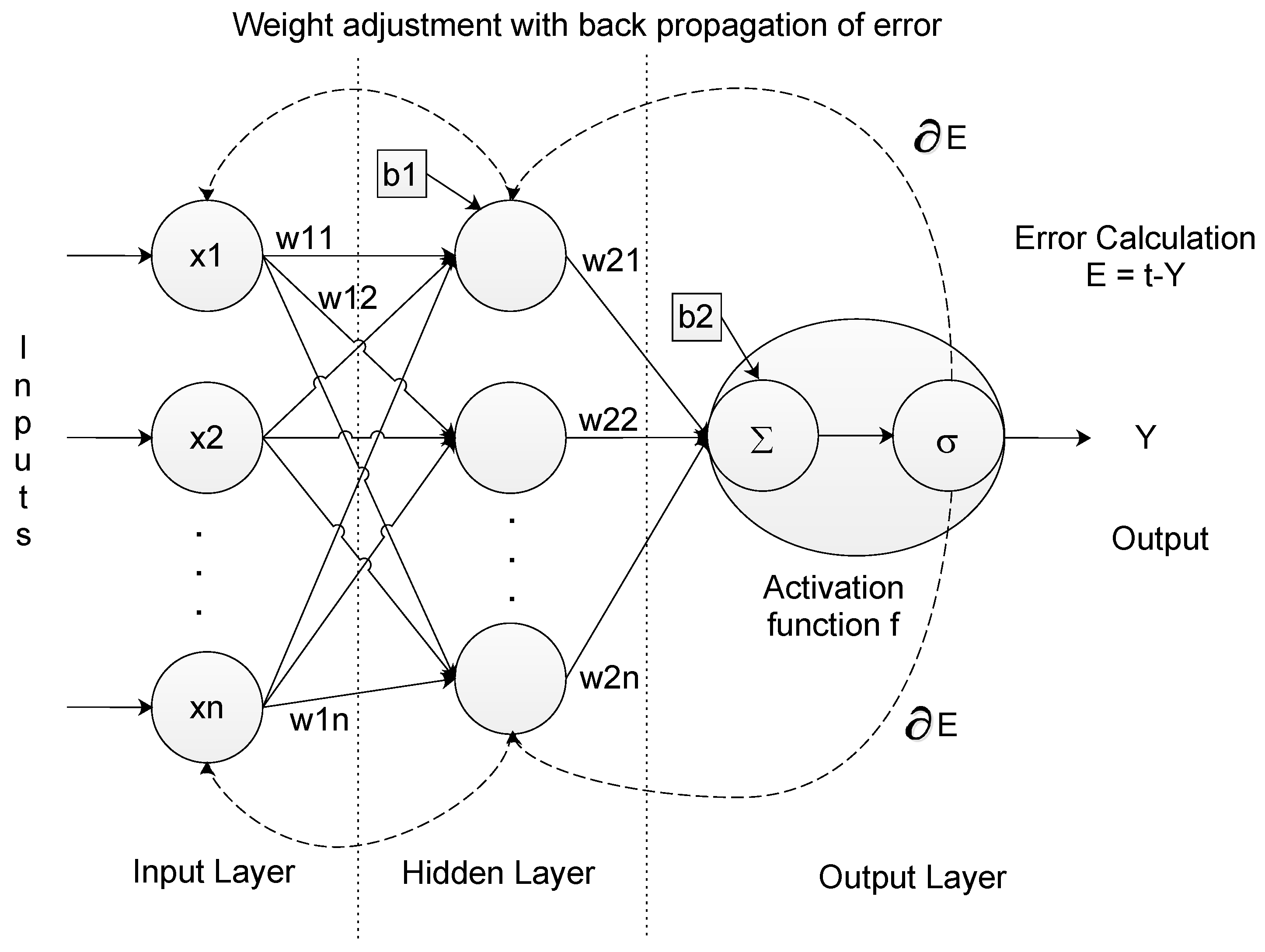
Figure 1. Backpropagation artificial neural network with gradient descent weight updating.
Sustainability 11 00987 g001
Figure 2. Architecture of one unit of LSTM [44].
Sustainability 11 00987 g002
Figure 3. Proposed system model.
Sustainability 11 00987 g003
Figure 4. Flowchart of proposed forecasting method.
Sustainability 11 00987 g004
Figure 5. Architecture of proposed method, DLSTM.
Sustainability 11 00987 g005
Figure 6. Error drop of MAE with addition of hidden layers in DLSTM network.
Sustainability 11 00987 g006
Figure 7. Network stability with epochs.
Sustainability 11 00987 g007
Figure 8. Normalized load of ISO NE, January 2011 to March 2018.
Sustainability 11 00987 g008
Figure 9. Normalized price of ISO NE, January 2011 to March 2018.
Sustainability 11 00987 g009
Figure 10. Relation between load and price signals of ISO NE, January 2011 to March 2018.
Sustainability 11 00987 g010
Figure 11. Normalized load of NYISO, January 2001 to March 2018.
Sustainability 11 00987 g011
Figure 12. Normalized price of NYISO, January 2006 to March 2018.
Sustainability 11 00987 g012
Figure 13. Relation between load and price signals of NYISO, January 2006 to March 2018.
Sustainability 11 00987 g013
Figure 14. (a) The normalized price of January 2017; (b) the normalized price of January 2018; (c) the normalized price of March 2017; and (d) the normalized price of March 2018.
Sustainability 11 00987 g014
Figure 15. Forecasted price of one day, ISO NE.
Sustainability 11 00987 g015
Figure 16. Forecasted price of one week, ISO NE.
Sustainability 11 00987 g016
Figure 17. Forecasted load of one day, ISO NE.
Sustainability 11 00987 g017
Figure 18. Forecasted load of one week, ISO NE.
Sustainability 11 00987 g018
Figure 19. Forecasted price of one day, NYISO.
Sustainability 11 00987 g019
Figure 20. Forecasted price of one week, NYISO.
Sustainability 11 00987 g020
Figure 21. Forecasted price of one month, NYISO.
Sustainability 11 00987 g021
Figure 22. Forecasted load of one day, NYISO.
Sustainability 11 00987 g022
Figure 23. Forecasted load of one week, NYISO.
Sustainability 11 00987 g023
Figure 24. Forecasted load of one month, NYISO.
Sustainability 11 00987 g024
Figure 25. Comparison of DLSTM, ELM and NARX for price forecast of one week, ISO NE.
Sustainability 11 00987 g025
Figure 26. Comparison of DLSTM, ELM and NARX for load forecast of one week, ISO NE.
Sustainability 11 00987 g026
Figure 27. Comparison of DLSTM, ELM and NARX for price forecast of one month, NYISO.
Sustainability 11 00987 g027
Figure 28. Comparison DLSTM, ELM and NARX for load forecast of one month, NYISO.
Sustainability 11 00987 g028
Table 1. Related work of load and price forecasting.
TaskForecast HorizonPlatform/TestbedDatasetAlgorithms
Load forecasting [13]Short-termHourly data of 6 states OF USANYISO 2015DWT-IR, SVM, Sperm whale algorithm
Load forecasting [14]Short-termHourly price of PJMPJM, 2016–2017Weighted voting mechanism
Load and price forecasting [18]Short-termHourly data New South Wales, New YorkNYISO, PJM, AEMO, 2012, 2014, 2010FWPT, NLSSVM, ARIMA, ABC
Price forecasting [21]Short-termHourly data of 6 states of USAISO NE, 2010–2015GCA, Random forest, ReliefF, DE-SVM
Load forecasting [22]Short-termElectricity market of three USA grids: FE, DAYTOWN, and EKPCPJMModified Mutual Information (MI), ANN
Price forecasting [23]Short-termOntario electricity marketAEMO, 2014ELM based improved WNN
Load forecasting [24]Short-termElectricity market data of 3 USA gridsPJM, 2014Modified MI, ANN
Load forecasting [25]Short-termHalf hour cooling consumption data of a educational buildingHong Kong, 2015Deep auto-encoders
Load forecasting [26]Short-termKoreaKorea Electric Power Company, 2012–2014DNN, RBM, ReLU
Load forecasting [27]Short-termHourly load and weather data of four regionsLos Angeles, California, Florida and New York City, July 2015–August 2016Stacked de-noising auto-encoder, SVR
Load forecasting [28]Short-term15 min consumption dataSingle user high consumption data from Foshan, Guangdong province of China, March–May 2016Trend index, auto-encoder
Load forecasting [29]Short-termIreland consumptionLoad profiles database of IrelandPooling deep RNN
Load forecasting [30]Medium-termFranceHalf hourly metropolitan electricity load, 2008–2016LSTM, GA
Price forecasting [31]Medium-termHourly load of 5 hubs of Midcontinent Independent System Operator (MISO)MISO USA, 2012–2014Stacked de-noising autoencoder
Price forecasting [32]Short-termHourly Turkish day-ahead electricity marketTurkey, 2013–2016Gated recurrent network
Price forecasting [33]Short-termHalf hour regulation market capacity clearing priceElectric power markets (PJM), 2017CNN, LSTM
Load forecasting [36]Short-termEight buildings of a public university15 min consumption, 2011–2017K-means clustering, Davies–Bouldin distance function
Consumption and peak demand forecasting [37]Medium-termEntertainment venues of OntarioDaily, hourly and 15 min energy consumption, 2012–2014ANN, SVR
Demand forecasting [38]Short-term21 zones of USATemperature, humidity and consumption data, 2004–2007Recency effect model without computational constraints
Table 2. Monthly forecasting error of energy price.
DataISO NENYISO
MonthJanuaryFebruaryMarchAprilJanuaryFebruaryMarchApril
MAE1.721.452.71.923.63.82.92.7
NRMSE0.0760.0620.1020.0820.0320.0430.0370.047
MonthMayJuneJulyAugustMayJuneJulyAugust
MAE2.831.451.961.922.142.72.422.56
NRMSE0.1070.0620.0870.1020.0140.0170.0240.031
MonthSeptemberOctoberNovemberDecemberSeptemberOctoberNovemberDecember
MAE2.041.362.011.982.192.362.82.12
NRMSE0.0930.0570.1240.1150.0470.0140.0180.021
Table 3. Comparison of load and price forecasting errors.
ForecastDataISO NENYISO
Forecasting MethodMAENRMSEMAENRMSE
ELM67.411.869.977.36
Price ForecastNARX12.478.2410.328.62
WT+SAPSO+KELM [46]8.990.1319.260.06
DLSTM1.9450.082.60.028
ELM52.88.429.685.24
Load ForecastNARX37.1814.7412.3611.57
INARX [47]9.70.21.90.02
DLSTM2.90.0871.40.012
Table 4. Diebold–Mariano test results and Friedman tests’ F ranks.
DataISO NENYISO
ForecastForecasting MethodDiebold–MarianoFriedmanDiebold–MarianoFriedman
DLSTM vs.F RankDLSTM vs.F Rank
Price ForecastELM47.3452.64
NARX27.6321.43
WT+SAPSO+KELM [46]12.828.62
DLSTMN/A1N/A1
Load ForecastELM43.2334.74
NARX6.827.93
INARX [47]4.223.82
DLSTMN/A1N/A1