Article

Characteristics Analysis of Freight Mode Choice Model According to the Introduction of a New Freight Transport System

Department of Logistics Research, The Korea Transport Institute, Sejong-Si 30147, Korea
*
Author to whom correspondence should be addressed.
Sustainability 2019, 11(4), 1209; https://doi.org/10.3390/su11041209
Submission received: 22 January 2019 / Revised: 12 February 2019 / Accepted: 20 February 2019 / Published: 25 February 2019
(This article belongs to the Special Issue International Freight Transport & Logistics)

Abstract

:
The purpose of this study is to identify the characteristics of freight mode choices made by shippers and carriers with the introduction of a new freight transport system. We set an area in which actual freight transport takes place as the analysis scope and performed a survey of the shippers and carriers that transport containers to identify their stated preference (SP) regarding the new freight mode. The SP survey was carried out through an experimental design and this study considered the three factors of transport time, transport cost, and service level. This study compared and analyzed the models by distance using an individual behavior model. The results of estimating the model showed that the explanatory power of the model classified by distance and the individual parameters have statistical significance. The hit ratio was also high, which confirms that the model was estimated properly. In addition, the range of elasticity and the value of travel time analyzed using the model were evaluated to be appropriate compared to previous studies. The findings of the elasticity analysis show that strategies for reducing the transport cost are effective to increase the demand for the new transport mode. The value of travel time of freight transport was found to be higher than the current value generally applied in Korea. Considering that the value of travel time currently used is based on road freight transport, further research is required to apply a new value of travel time that reflects the characteristics of the new transport mode in the future.

1. Introduction

In 2015, the modal share of freight transport in Korea (based on ton-km) was 76.2% for roads, 18.4% for shipping, 5.3% for railways, and 0.1% for air transport, showing that road transport dominated compared to other means of transport. In addition, transport costs accounted for 71.1% of the nation’s logistics costs in 2015 [1,2]. Structural problems continued to increase because of the extremely high proportion of road transport in the freight transport process. Such structural problems include increased inland transport costs, increased traffic congestion costs, increased air pollution and noise, maintenance required due to road damage, and serious traffic accidents caused by freight trucks.
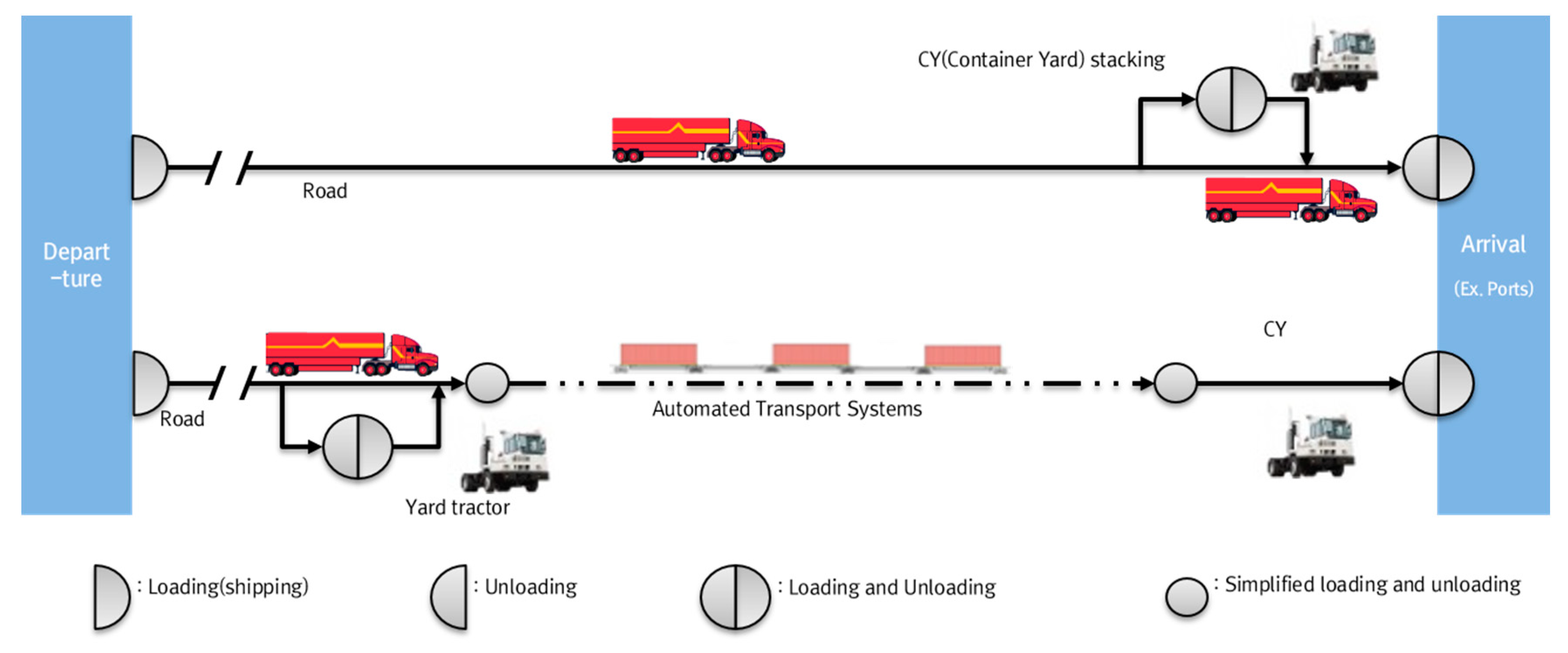
Currently, the land freight transport system can be divided into railway transport, which has not changed much in terms of shape over 250 years, and truck transport, which has a history of about 100 years. However, the need for new freight transport modes, including the intermodal automated freight transport system, in order to overcome the structural limitations of land freight transport has been emerging worldwide.
In Europe and the US, the development of various types of new-concept transport system technologies began in the early 2000s. Recently, these countries have been on the verge of commercialization as they have entered the stage of verifying the developed technologies, such as through operating test beds of the newly developed transport systems. In particular, technically advanced countries such as the US, Germany, the Netherlands, and Japan are developing various types of intermodal automated freight transport systems, including automated freight transport systems for bulk cargo between logistics hubs and underground freight transport systems [3,4,5]. Typical technologies in this area include Freight Shuttle System, CargoRail Tram, CargoCap, TubeXpress (SUBTRANS), SkyTech, Cargo Tunnel, and UCM [6]. In Korea, the development of an intermodal automated freight transport system technology (Phase 1; development name: AutoCon III), which received support from the Ministry of Land, Infrastructure, and Transport’s (MOLIT’s) Transport and Logistics Development Research Project, started on June 2017, so we expect the relevant technologies to be commercialized in the near future [7]. However, we lack the information and data to make policy decisions, as there has been insufficient research to forecast changes in the transport environment and the modal split due to introducing new systems independent of technology development.
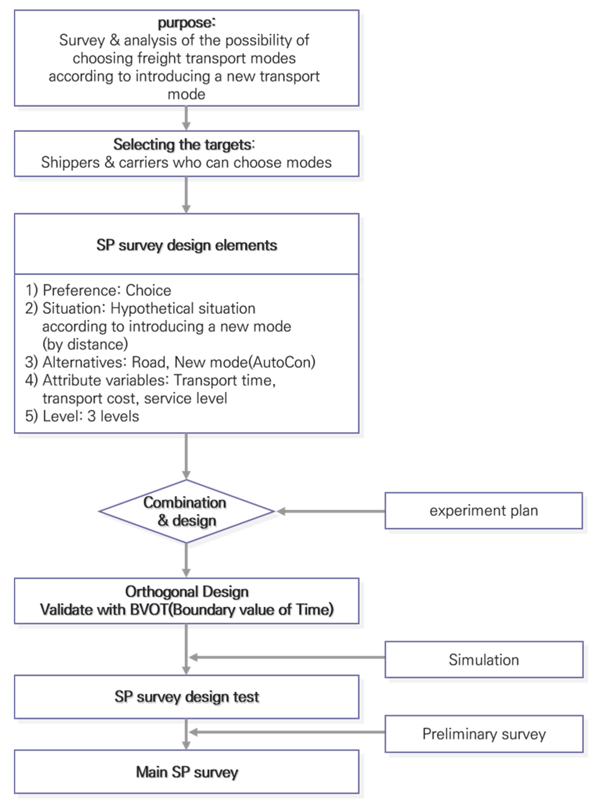
As such, the purpose of this study is to analyze the characteristics of the process shippers and carriers in Korea used in choosing freight transport modes and to identify the conditions and ratio of the modal share structure between the new system of transport and truck transport after introducing the intermodal automated freight transport system to provide the basic data required for the policy-making process. Therefore, this study considers changes in the transportation environment assuming the introduction of a new freight transport mode (intermodal automated freight transport system) which does not currently exist and performed a stated preference (SP) survey to identify changes in the perception of the shippers and carriers in the freight transport market. Section 2 presents the differentiation of this study through a consideration of previous studies and Section 3 summarizes the process used to collect the data required to build a freight mode choice model. Section 4 builds a freight transport mode choice model according to the introduction of a new freight transport system using the collected data, while Section 5 analyzes the characteristics of the choices of freight transport means by the shippers and carriers using the model. Finally, Section 6 presents the conclusions drawn from the study and the limitations of this study.

2. Consideration of Previous Studies

In Korea, there have only been a few studies on the mode choice model related to freight transport and it is difficult to find studies that have built a mode choice model for new transportation modes (Table 1). Studies that estimate the freight mode choice model in Korea can be classified according to the transport mode and data type. First, the studies that analyze the difference according to the transport mode can be divided into studies that analyze the competitive relationship between commercial and private trucks in road transport [8,9,10] and studies that analyze the competitive relationship between transport modes such as roads, railways, and shipping [11,12,13,14]. Meanwhile, if we classify the previous studies based on the type of data, they can be divided into studies that use revealed preference (RP) data to investigate the actual situation [9,10] and studies that use SP data to implement hypothetical choices [8,11,12,13,14]. RP survey is intended to identify preferences and demands for existing modes and SP survey is for new modes that do not currently exist.
Recent studies have identified preferences for new transport modes on the basis of hypothetical conditions and have identified a modal share structure for existing modes [11,12,13]. Lee et al. (2009) conducted SP surveys for container, steel, and hazardous materials cargos to find the utility function for dual mode trailer (DMT) [11]. Choi et al. (2008) conducted SP surveys for container, cement, and steel cargos under the actual transportation environment, and defined mode choice character [12]. Kim et al. (2008) conducted SP surveys for container and bulk cargo according to changes in transportation time, transportation cost, trans-shipment time, trans-shipment cost, shuttle time, and shuttle cost [13]. Choi and Lim (1999) and The Korea Transport Institute (KOTI) (1998) [9,10] conducted large-scale RP surveys on shippers to identify preferences and demand for existing alternatives.
In other countries, research has been performed for more diverse purposes compared to the research in Korea, such as research techniques, methodologies, competition by modes, and analysis areas. Studies that applied the SP survey techniques to freight transport include Norojono et al. (2003), Shinghal et al. (2002), and Fowkes et al. (1991) [15,16,17] and methods of integrating SP and RP data to apply them to model estimation have been attempted in the study by De Jong et al. (2001) [18]. In terms of methodology, all of the studies in Korea used logit models, while disaggregate logit models and multiple regression models were used in other countries. Different from the traditional four-step travel demand model, the logit model is a probabilistic choice model which can analyze individual mode choice characteristics because it is estimated using the disaggregate data. The logit model is based on the theory of selective behavior, which is in turn based on the microeconomic consumer theory. The estimation coefficient of the logit model is widely used in the construction of the mode choice model because it is easy to interpret the marginal utility of each explanatory variable. De Jong and Ben-Akiva (2007) used a logit model to analyze the composite transport network when considering a non-selective alternative set of one million alternatives from the Swedish freight volume data [19]. Ham et al. (2005) applied a linear regression model to estimate the coefficient of the logit model using US freight volume survey data for a mode choice model considering road and rail [20]. Bolis and Maggi (2003) investigated Italian and Swiss companies and demonstrated through a logistic regression model that railways can be competitive against road transport by improving the on-time arrival rate [21]. In terms of case studies on the competitive relationship between roads and railways, Norojono et al. (2003) analyzed the modal share characteristics of roads and railways in Indonesia and proposed measures to increase the use of railway logistics and Shinghal et al. (2002) configured a competitive relationship between roads and railways to study the factors of freight mode choice in India [15,16]. All of the three studies mentioned above used SP survey data and logit models.
Although technologies for new freight transport systems are being developed all over the world, there are only a few cases in which freight mode choice models have been built that apply to new freight transport systems in Korea and in other countries. For this reason, it is necessary to develop a new freight mode choice model that reflects changes in the freight transport environment, such as new freight transport systems, to identify the characteristics of choosing the freight transport modes required to make policy decisions on freight transport systems.

3. Collecting Research Data

3.1. SP Survey Design

The individual behavior model is the appropriate model for the research objective to identify the transport mode choice characteristics of shippers. Since the individual behavior model uses disaggregate data, it can reflect the mode choice characteristics of each shipper in the model. This study applied the logit model, which is the most widely used model to configure transport mode choices. Since the data used in the study is intended to reflect changes in the transport environment related to introducing new freight transport modes and to grasp the characteristics of the shippers in a diversified freight transport market, we decided that SP data was more appropriate than RP data.
The SP survey design was oriented toward building a new freight transport mode split model by researching and analyzing the possibility of selecting a transport mode after introducing a new freight transport system as shown in Figure 1. The SP survey provides individual respondents with alternatives composed of hypothetical situations, each of which consists of factors such as transport cost and time, which represent the mode choice characteristics. For the given alternatives, the respondents may rank, rate, or choose their preferred alternatives. The choice method was widely used in previous studies, so this study used the same method. However, the SP survey was performed by considering the limitations of potential response errors during the investigation process due to composing hypothetical scenarios.
The SP survey period was from July to September 2018. As shown in Figure 2, the survey was limited to shippers and carriers that use Busan New Port and handle containers based in Busan, Ulsan, and South Gyeongsang Province, which are areas near Busan New Port, which is expected to introduce the new freight transport system.
As shown in Figure 3, the SP survey was performed by the respondents choosing a preferred alternative between the two alternatives of road transport mode and the new freight transport mode. The four optional alternatives for freight transport mode include rail transport, road transport, coastal shipping, and air transport. However, since the function of the intermodal automated freight transport system is limited to shuttle transport connecting the port and surrounding areas, the modal share of rail transport, coastal shipping, and air transport is not expected to change even if a new freight transport system is introduced, so this study set two alternatives.
The choice situation was set according to the transportation distance for connecting the production hub and international logistics hub in the target area. The choice of transport mode may vary depending on the freight transport distance. Therefore, this study investigated the actual transport environment of import and export container items in order to identify the characteristics of choosing modes that vary depending on the representative transport distance. The transport condition was assumed to be one-way transport of one 40 ft container (1 forty-foot equivalent unit (FEU) or 2 twenty-foot equivalent unit (TEU)). Transport distances were divided into distances less than 20 km and distances more than 20 km, taking into account considered route alternatives between Busan New Port and the international industrial logistics complex in the hinterland of the port. This study selected transport cost, transport time, and service level (a significant non-quantitative factor in the freight transport process) as the attribute variables, as these were found to be most important in the freight mode choice models of previous studies. The service level was defined to include the reliability of arriving at the destination at a given time, availability of use when needed, safety of freight transport against damage or loss, convenience of providing information about the location or arrival of cargo, connectivity with other modes, and the potential to smoothly handle future increases in trade volume. The investigators explained these points for the understanding of the participants before the survey. The service level was quantified by dividing the cases into 100% when satisfied, 80% when normal, and 60% when unsatisfied. We used a three-level orthogonal arrays table in the design of the SP survey. Furthermore, the lower limit was set at −20% to reflect the survey finding that carriers and shippers, who were not willing to switch at the time of introducing the new transport mode, were willing to switch when the transport cost, transport time, and service level dropped by 20%. In addition, the upper limit is set to +10% referring to a previous study [12] and level 3, assuming that the transport cost, transport time, or service level will be further increased or improved. The reference value of road transport cost and time were classified into the on-board transport cost and the cost of loading and unloading. First, the on-board transport cost was set as half (84.01 USD) of the round-trip fare (168.03 USD) of Busan New Port based on the 40 ft land transport rate announced by the Korea Trucking Association (2013) [23] and the cost of loading and unloading was set as 53.34 USD per unit, reflecting the market price of Busan New Port. In addition, the on-board transport time was calculated as 1.18 hours per trip (71 minutes) using the average number of container shuttle operations per day (6.5 times) and average operation hours per day (7.7 hours), according to the freight transport market trend in 2017 (third quarter). In terms of the loading and unloading time, we confirmed that 18–25 containers are processed per hour in the field, but this study assumed that 15 containers are handled per hour, so the total time required to load and unload one container is 8 minutes (4 minutes each for origin and destination). In terms of the transport costs of the new transport system, we assumed that the cost of loading and unloading would be the same, while the on-board transport cost would be 90% of the road on-board transport cost. The transport time was calculated as the sum of the on-board transport time, the access/egress from the origin to the terminal and from the terminal to the destination, terminal operating time, and the waiting time. The on-board transport time was assumed to be 40 minutes when traveling the average distance of road transport at 50 km/h, the access time to the terminal was 15 minutes, and the terminal operating time and waiting time were each assumed to be 20 minutes. Table 2 summarizes the levels by attribute variable for each alternative.

3.2. Collecting Research Data

As mentioned above, the SP survey of this study is composed into the preliminary survey and the first and second surveys, as shown in Table 3. In the preliminary survey, 50 samples were collected for the purpose of revising and supplementing the questionnaire and selecting the survey target. In the first survey, 50 samples were checked to confirm whether the modified questionnaire worked and, after confirming the questionnaire, the second survey of 250 samples was conducted. Among the 350 companies surveyed, 206 companies (59.0%) were carriers and 143 companies (41.0%) were shippers.
The main survey was carried out after supplementing and revising the questionnaire following a preliminary survey. Considering the difficulty involved in answering the survey, the investigators visited the participants in person to explain and receive answers. After collecting the questionnaires, we excluded questionnaires that simply repeated the same response or had logically contradictory answers; here, logically contradictory answers refers to surveys in which the participant did not respond to several types of questions presented in the SP experiment, such as when the participant did not fully understand the SP experiment or when the participant had a fixed choice and did not consider the context of the transport mode. We also excluded cases in which personal attribute data, such as the age of the participant and the freight size, were omitted. Table 4 summarizes the data collected through the process above; market segmentation was performed according to the transport distance.

4. Estimating the Freight Transport Mode Choice Model

4.1. Model Configuration

This study used a logit model as an individual behavior model to estimate the demand for switching freight based on the disaggregate data. The market was segmented according to the freight transport distance; the model is shown in Table 5. The utility function consisted of transport time, service level, and transport cost as the explanatory variables and the model was configured so that the relative utility of the new transport mode for road transportation can be identified by setting truck transport as a reference.

4.2. Model Estimation and Testing the Results

4.2.1. Model Estimation and Significance Test

Table 6 shows the results of estimating the mode choice model according to Table 5. First, the likelihood ( ρ 2 ), which indicates the goodness-of-fit of the model, was between 0.32 and 0.41, ensuring a certain level of significance depending on the model. Typically, if the likelihood ( ρ 2 ) has a value in the range of 0.2–0.4, the model is usually evaluated to be significant [24]. In general, the mode choice model of freight transport tends to have a lower likelihood than that of passenger transport, because the entities that make up the passage are more complex and lack homogeneity compared to passenger transport. In addition, both the statistical significance (t-value) of the individual parameters and the sign of utility were found to be appropriate. The AutoCon dummy variable has a (+) value, which indicates that the new freight transport mode was preferred over conventional truck transport. These results suggest that the new transport mode has the potential to gain a competitive advantage over road transport.

4.2.2. Testing the Results of Market Segmentation According to the Transport Distance

Table 7 shows the hypothesis test results for comparing the individual parameters for the models classified according to the transport distance. For transport distances less than 20 km and more than 20 km, we can confirm that, with the exception of the transport cost, none of the explanatory variables are statistically different from each other.
We could confirm the statistical significance by testing the hypothesis for comparing the whole model in market segmentation by distance using Model 1, which used the full data set, and Models 2 and 3, which used market segmentation by distance [25]. First, the null hypothesis (H0) and the alternative hypothesis (H1) were set as follows in order to comprehensively compare the estimation results of the model by market segmented subgroups.
Hypothesis 0.
H0: β1 = β2 = … = βx
Hypothesis 1.
H1: Not all βx’s are the same
Here, βx is the vector of coefficients for the market segmented subgroup x by distance. The test statistic used to test this hypothesis is statistic, and the equation is as follows.
X 2 = 2 [ L N ( β ^ ) x = 1 2 L n x ( β ^ x ) ] ,
where L N ( β ^ ) : Log-likelihood function value at the maximum value of the log-likelihood function when using the whole data and   L n x ( β ^ x ) : log-likelihood function value at the maximum value of the log-likelihood function when using the sample data of the market segmented subgroups.
With the likelihood test statistic ( X 2 ) 14.2578, which was calculated from the hypothesis test for comparing the whole model in the market segmentation by distance, the null hypothesis was rejected at a significance level of 0.5% and 4 degrees of freedom, so the difference in the vector of the estimated coefficient values between the two groups was clearly significant.

4.2.3. Final Model

This study set the final model as shown in Table 8 through a model estimation process and a statistical testing procedure. The model corresponds to Model 2 and Model 3 in Table 4, and is classified according to the transport distance. This study presents a model by dividing the mode choice model by distance according to the introduction of a new freight transport mode. In addition, it seems reasonable to present a separate model for each item since the absolute values of the individual coefficients are different, which results in different elasticities.

5. Evaluating the Applicability of the Model and Interpreting the Results

The model estimated in this study can be applied not only to analyze how new freight modes and trucks change the mode split depending on the competition conditions, but also to provide the basic data required for the process of making policy decisions using models. Elasticity is generally used in the policy-making process and the value of travel time is also used as an index to evaluate the importance of freight transport or the economic feasibility of transport facility investment projects.

5.1. Evaluating the Predictive Power and Applicability of the Model

By using the estimated model, we can predict how the modal split will change as the transportation environment changes. For example, when there is a cost change in each transport mode, we can use the model to calculate the new modal split. To accomplish this, we first need to assess how well the estimated model reflects reality. This study uses the hit ratio to achieve this, as the hit ratio refers to the ratio in which the transport mode predicted in the model matches the actual chosen transport mode. Table 9 shows the results of calculating the hit ratio for the optimal model, showing a value between 80.5% and 77.8%.

5.2. Scope of Elasticity and Applicability of Evaluating Policy

Elasticity refers to the degree of change in demand for changes in the explanatory variables and in the freight transport process, the elasticity of transport cost or time is measured for use as data in determining policies. Table 10 shows the elasticity results calculated in this study. Looking at prior studies that estimate the elasticity of freight items in other countries, Winston (1981) proposed a cost elasticity (−0.04 ~ −2.97) and a time elasticity (−0.15 ~ 0.69) for road transport and a cost elasticity (−0.08 ~ −2.68) and a time elasticity (−0.07 ~ 2.33) for railway transport [26]. Since there are no items directly comparable to this study, we can only compare a rough distribution. In terms of the value of travel time of freight transport in the study by Small and Winston (1999), the transport cost was −0.04 ~ −2.97 for roads, −0.08 ~ −2.68 for railways, and the transport time was −0.15 ~ −0.69 for roads and −0.07 ~ −2.33 for railways [27]. Looking at the domestic case studies, the elasticity of container transport was studied by Ha et al. (1996) and Choi et al. (2008). In the study by Ha et al. (1996), the elasticity of container transport cost was railway (−3.46) and road (−3.81) and the transport cost was railway (−1.90) and road (−1.44) [14]. In addition, in the study of Choi et al. (2008), the elasticity of transport cost was railway (−2.88) and road (−4.38) and the elasticity of transport time was railway (−1.43) and road (1.74); thus, the elasticity of transport cost was higher than that of transport time [12]. However, both domestic and foreign studies have no data on containers, and have also not established a mode choice model for new transport modes, making it difficult to make an accurate comparison. Table 10 shows the elasticity by model, in which the transport costs in all models regardless of distance was found through an analysis to be much higher than the elasticity of transport time or service level. These results show that reducing fares is a great way to increase freight demand.

5.3. Estimating the Value of Travel Time and Implications

The value of travel time of freight transport can be interpreted as the monetary cost that the shipper or carrier is willing to sacrifice to reduce transport time by one unit. In the model, it is calculated as the ratio between the time parameter and the cost parameter. As shown in Table 11, the value of travel time was calculated to be 22.43 USD/unit for less than 20 km and 25.67 USD/unit for more than 20 km.
In Korea, the value of travel time applied to the economic feasibility evaluation is calculated by using the truck driver’s wage level, which is 14.73 USD/unit at the time of this study and 15.29 USD/unit when adjusted by reflecting the consumer price index of 2017 [28]. In Japan and the US, the value of travel time includes the inventory value of the freight in transit and the opportunity cost of the truck in addition to the driver’s wage. Particularly in Japan, the value of travel time for freight transported by railway is larger than the value estimated using the wage rate method because it is estimated separately by using SP. In this study, considering the fact that it is a new freight transport mode and working on the premise that the value of travel time of the new freight transport system to be developed will be higher than that of road transport, we can confirm that the derived values are reasonable.

6. Conclusions

This study developed a new freight mode choice model based on the introduction of a new freight transport system. This is due to the need to develop a separate transport mode choice model according to the introduction of the new transport mode. For this purpose, we investigated the stated preference of the new transport mode for shippers and carriers who actually transport containers. We used the individual behavior model and SP survey data. The SP survey used to acquire data was prepared through experimental design and the attribute variables were transport time, service level, and transport cost. In addition, this study tried to analyze the models by distance. Through this analysis, it was found that the explanatory power and the individual parameters of the model classified according to distance were statistically significant. It also showed a high hit ratio, which proved that the developed model was appropriate. Also, the range of elasticity and the value of travel time were evaluated to be appropriate compared to previous studies. By analyzing the elasticity, this study confirmed that strategies for reducing the transport cost were more effective than strategies for reducing transport time or increasing the service level in order to increase the demand for the new transport mode.
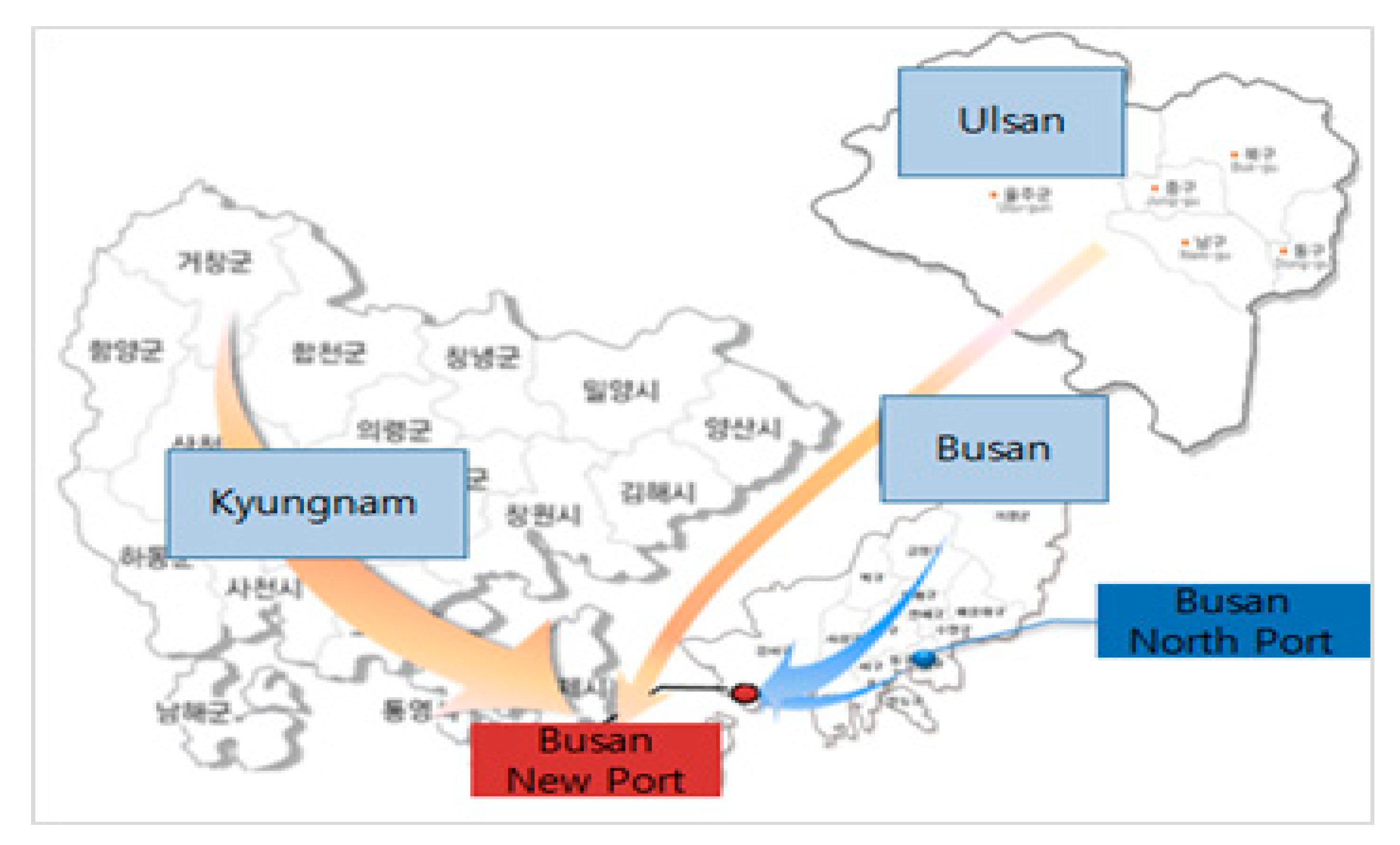
Although this study is meaningful in that it established a freight mode choice model to estimate the freight volume that could be converted from the traditional transport system to the new system after introducing a new automated freight transport system, the research had the following limitations, which need to be addressed in future studies. First, though the changes in freight traffic patterns when introducing a new freight transport system should be considered, this study performed the survey centered around areas near Busan New Port without configuring a separate area of influence. Second, the freight value of travel time estimated in this study was higher than the current value of travel time applied in Korea. Considering that the current value of travel time is based on road transport freight, we need to find a way to apply an estimated value of travel time by reflecting the characteristics of the new transport mode. Third, the transport distance was divided into less than 20 km and more than 20 km through assumption when segmenting the market of the model, but further studies are needed to segment the transport distance by analyzing the competitiveness of the two transport modes by distance. Finally, this study developed a freight mode choice model based on the introduction of a new transport mode, but the developed freight mode choice model has not yet been applied to the real world. We hope that future studies will address these limitations.

Supplementary Materials

Supplementary File 1

Author Contributions

For research articles with several authors, a short paragraph specifying their individual contributions must be provided. The following statements should be used “Conceptualization, S.S. and S.H.H.; Methodology, S.S.; Software, S.S.; Validation, S.S., S.H.H. and H.-S.R.; Formal Analysis, S.S.; Investigation, H.-S.R.; Resources, S.H.H.; Data Curation, S.S and S.H.H.; Writing-Original Draft Preparation, S.S.; Writing-Review & Editing, S.H.H.; Visualization, S.H.H.; Supervision, H.-S.R.; Project Administration, H.-S.R.; Funding Acquisition, H.-S.R.”.

Funding

This research was supported by a grant from “Transportation logistics research Program (18TLRP-B134108-02),” funded by Ministry of Land, Infrastructure and Transport of Korean Government (MOLIT).

Conflicts of Interest

The authors declare no conflict of interest.

References

  1. The Korea Transport Institute (KOTI). National Transportation Demand Survey and Database Establishment in 2015: Expanded Nationwide Freight O/D through Supplementation and Updates; The Korea Transport Institute: Sejong-si, Korea, 2016. [Google Scholar]
  2. Kwon, H.; Seo, S.; Kwon, T. Korean National Logistics Costs in 2015; Policy Research Reports; The Korea Transport Institute: Sejong-si, Korea, 2017. [Google Scholar]
  3. Van Binsbergen, A.J.; Konings, R.; Tavasszy, L.A.; van Duin, J.H.R. Innovations in intermodal freight transport: Lessons from Europe. In Proceedings of the the 93th Annual Meeting of the Transportation Research Board, Washington, DC, USA, 12–16 January 2014. [Google Scholar]
  4. Roh, H.S.; Oh, J.H.; Jung, S.J.; Moon, J.S.; Min, Y.J.; Jang, S.Y. A Technical Study on the Automated Container Transport System (AutoCon) betweem Seoul and Busan in Korea; Basic Research Reports; The Korea Transport Institute: Sejong-si, Korea, 2010. [Google Scholar]
  5. Rijsenbrij, J.C.; Pielage, B.A.; Visser, J.G.S.N. State-Of-The-Art on Automated (Underground) Freight Transport Systems for the EU-TREND Project; Delft University of Technology: Delft, The Netherlands, 2006. [Google Scholar]
  6. Shin, S.; Roh, H.S.; Hur, S.H. Technical Trends Related to Intermodal Automated Freight Transport Systems (AFTS). Asian J. Shipp. Logist. 2018, 34, 161–169. [Google Scholar] [CrossRef]
  7. Korea Agency for Infrastructure Technology Advancement. A Technology Development on Automated Intermodal Freight Transport System (Phase 1); KAIA: Anyang-si, Korea, 2017. [Google Scholar]
  8. Choi, C. A Study on Estimating the Value of Travel Time of Freight Transportation for Toll Roads Investment Evaluation. J. Korea Plan. Assoc. 2004, 43, 109–125. [Google Scholar]
  9. Choi, C.; Lim, K. Development of A Behavioral Mode Choice Model for Road Goods Movement. J. Korea Plan. Assoc. 1999, 34, 103–115. [Google Scholar]
  10. The Korea Transport Institute (KOTI). Establishment of a Basic Plan for Construction of National Railway Network in the 21st Century; KOTI: Sejong-si, Korea, 1998. [Google Scholar]
  11. Lee, K.-W.; KooK, K.-H.; Jang, S.-Y. Estimation of the DMT Utility Function Using SP Survey. J. Korean Soc. Railw. 2009, 12, 348–356. [Google Scholar]
  12. Choi, C.; Shin, S.; Park, D.; Kim, H.; Jin, J. Mode Choice Characteristics of Rail Freight Transportation. J. Korean Soc. Railw. 2008, 11, 588–595. [Google Scholar]
  13. Kim, C.; Lee, J.; Jung, K. A Study on Intercity Freight Mode Choice Modelling; Policy Research Reports; The Korea Transport Institute: Sejong-si, Korea, 2008. [Google Scholar]
  14. Ha, W.; Nam, K. Mode Choice Models for Freight Transportation Using SP Data. J. Korea Transp. Res. Soc. 1996, 14, 81–99. [Google Scholar]
  15. Norojono, O.; Young, W. A Stated Preference Freight Mode Choice Model. Transp. Plan. Technol. 2003, 26, 195–212. [Google Scholar] [CrossRef]
  16. Shinghal, N.; Fowkes, T. Freight mode choice and adaptive stated preferences. Transp. Res. Part E 2002, 38, 367–378. [Google Scholar] [CrossRef] [Green Version]
  17. Fowkes, S.; Nash, A.; Tweddle, G. Investigating the Market for Inter-modal Freight Technologies. Transp. Res. A 1991, 25, 161–172. [Google Scholar] [CrossRef]
  18. De Jong, G.; Velly, C.; Houėe, M. A Joint SP/RP Model of Freight Shipment from the Region Nord-Pas de Calais. In Proceedings of the European Transport Conference, Homerton College, Cambridge, UK, 10–12 September 2001. [Google Scholar]
  19. De Jong, G.; Ben-Akiva, M. A micro-simulation model of shipment size and transport chain choice. Transp. Res. Part B Methodol. 2007, 41, 950–965. [Google Scholar] [CrossRef]
  20. Ham, H.; Kim, T.J.; Boyce, D. Implementation and estimation of a combined model of interregional, multimodal commodity shipments and transportation network flows. Transp. Res. Part B Methodol. 2005, 39, 65–79. [Google Scholar] [CrossRef]
  21. Bolis, S.; Maggi, R. Logistics Strategy and Transport Service Choices: An Adaptive Stated Preference Experiment. Growth Chang. 2003, 34, 490–504. [Google Scholar] [CrossRef] [Green Version]
  22. Korea Agency for Infrastructure Technology Advancement. A Technology Development Plan on Automated Intermodal Freight Transport System for Cost Saving and Freight Transport System Innovation; KAIA: Anyang-si, Korea, 2014. [Google Scholar]
  23. Korea Trucking Association. Container Road Transport Rates Table. 2013. Available online: http://www.kta.or.kr/ (accessed on 7 December 2018).
  24. McFadden, D. The Theory and Practice of Disaggregate Demand Forecasting for Various Modes of Urban Transportation; Institute of Transportation Studies, Working Paper No. 7623; University of California: Berkeley, CA, USA, 1976. [Google Scholar]
  25. Ben-Akiva, M.E.; Lerman, S.R. Discrete Choice Analysis: Theory and Application to Travel Demand; MIT Press: Cambridge, MA, USA, 1985; Volume 9. [Google Scholar]
  26. Winston, C. A Disaggregate Model of the Demand for Intercity Freight Transportation. Econometrica 1981, 49, 981–1006. [Google Scholar] [CrossRef]
  27. Small, K.; Winston, C. The Demand for Transportation: Models and Applications, Essays in Transportation Economics and Policy: A Handbook in Honor of John R. Meyer; Brookings Institution Press: Washington, DC, USA, 1999; pp. 11–55. [Google Scholar]
  28. KDI. A Manual for Preliminary Economic Feasibility Test for Road and Railway, version 5; Korea Development Institute: Sejong-si, Korea, 2008. [Google Scholar]
Figure 1. SP survey design process.
Sustainability 11 01209 g001
Figure 2. Spatial scope of SP survey.
Sustainability 11 01209 g002
Figure 3. Comparison of automated intermodal transport systems with conventional logistics systems from a logistics process perspective. Source: Korea Agency for Infrastructure Technology Advancement (2014) [22].
Sustainability 11 01209 g003
Table 1. Scope of analysis.
ResearchersCountryData TypeModelAlternativesVariables
Lee et al. (2009)KoreaSP *LogitRoad, rail, dual mode trailerCost, time, reliability
Choi et al. (2008)KoreaSPLogitRoad, railCost, time, service level (reliability, availability, safety, information provision)
Kim et al. (2008)KoreaSPLogitRoad, rail, shippingCost (trans-shipment, shuttle), time (trans-shipment, shuttle)
Choi (2004)KoreaSPLogitRoad (four types)Cost, time, punctuality
Choi and Lim (1999)KoreaRP **LogitRoad16 explanatory variables
KOTI (1998)KoreaRPLogitRoadCost, time
Ha et al. (1996)KoreaSPLogitRoad, railCost, time, punctuality
De Jong and Ben-Akiva (2007)Norway, SwedenRPLogitRoad, rail, water, airDistance-based link costs, time-based link costs, loading and unloading costs, access and egress costs, trans-shipment costs
Ham et al. (2005)USRPCombined modelRoad, railaverage value of shipments, average shipment distance
Norojono et al. (2003)IndonesiaHierarchical SPHEVM ***Rail, large truck, amall truckCost, time, quality, utility
Bolis and Maggi (2003)Italy, SwitzerlandASP ****Logistic regressionRoad, railCost, time, on-time arrival rate, No. of monthly shipments, minimum notification time for shipping order
Shinghal et al. (2002)IndiaSPLogitRoad, railCost, time, punctuality
This paperKoreaSPLogitRoad, AutoConCost, time, service level (reliability, availability, safety, convenience, connectivity, potential)
Note: * stated preference, ** revealed preference, *** heteroscedastic extreme value (HEV) choice model, **** adaptive stated preference.
Table 2. Scope of analysis.
LevelRoadNew Freight Transport System
Transport Cost (USD)Transport Time (h)Service Level (%)Transport Cost (USD)Transport Time (h)Service Level (%)
Level 1−20%152.561.05 60145.841.1660
Level 2Reference Value190.701.3280182.301.4580
Level 310%209.771.45100200.531.60100
Note: Based on the US Dollar and the Korean Won exchange rate (1124.8 won/USD) as of 7 February 2019.
Table 3. SP survey samples.
Goal SamplePerformance SampleRatio (%)
Preliminary Survey5050100.0
1st Main Survey504896.0
2nd Main Survey250251100.4
Total35034999.7
Table 4. Market segmentation and number of available data.
Less Than 20 kmMore Than 20 kmTotal
No. of Respondents123152275
No. of Available SP Data126415862850
Table 5. Market segmentation and number of available data.
Model TypeMarket SegmentationUtility Function
Model 1Total V i = β 0 + β 1 ( T I M E ) + β 2 ( S L ) + β 3 ( C O S T ) ,
where V i : Utility function (AutoCon, Truck); β 0 : Dummy; β 1 ~ β 3 : Parameter; TIME: Transport time; SL: Service level; COST: Transport cost
By DistanceModel 2Distance less than 20 km
Model 3Distance greater than or equal to 20 km
Table 6. The results of modeling.
Model 1Model 2Model 3
CoefficientStandard Errort-RatioCoefficientStandard Errort-RatioCoefficientStandard Errort-Ratio
AutoCon Dummy0.390970.079704.906 ***0.405250.116883.467 ***0.392320.108953.601 ***
COST−0.643900.02541−25.341 ***−0.732510.03829−19.129 ***−0.558270.03388−16.476 ***
TIME−1.710340.24757−6.909 ***−1.847940.36127−5.115 ***−1.612190.33960−4.747 ***
Level of service0.014960.002975.035 ***0.014310.004273.355 ***0.015240.004163.663 ***
L (*)−1215.7570−631.8402−576.3973
L (0)−1920.4897−1074.1270−845.7610
ρ 2 0.366950.411760.31849
ρ 2 ¯ 0.366060.41028 0.31632
Observations (n)285015861264
Note: * Significant level 90%; ** Significant level 95%; *** Significant level 99%.
Table 7. Test hypothesis of parameter on distance.
Model 2
(Less Than 20 km)
Model 3
(More Than 20 km)
Test Hypothesis of Parameter on Distance
ParameterStandard ErrorParameterStandard Error
COST−0.732510.03829−0.558270.03388−3.40759
SL−1.847940.36127−1.612190.33960−0.47546
TIME0.014310.004270.015240.00416−0.15454
Table 8. Selected mode choice model by distance.
ModelUtility Function
Model 2 U A u t o C o n =0.40525-0.73251∙COST+0.01431∙SL-1.84794∙TIME
U T r u c k = -0.73251∙COST+0.01431∙SL-1.84794∙TIME
Model 3 U A u t o C o n =0.39232-0.55827·COST+0.01524∙SL-1.61219∙TIME
U T r u c k = -0.55827∙COST+0.01524∙SL-1.61219∙TIME
Table 9. Hit ratio of selected mode choice models.
Model Log - Likelihood   Ratio   ( ρ 2 ) Hit Ratio (%)
Model 20.4117680.52
Model 30.3184977.77
Table 10. Elasticities by distances and modes.
ModelVariablesModeElasticity
AutoConTruck
Model 2TIMEAutoCon−1.0740.928
Truck1.543−1.345
SLAutoCon0.476−0.458
Truck−0.6630.66
COSTAutoCon−6.245.763
Truck8.091−9.354
Model 3TIMEAutoCon−0.8930.766
Truck1.3851.22
SLAutoCon0.476−0.46
Truck−0.7320.726
COSTAutoCon−4.4984.23
Truck6.379−7.36
Table 11. Value of travel time (VOT) by distance.
Model 2Model 3
ParameterTIME−1.84794−1.61219
COST−0.73251−0.55827
VOTwon/vehicle25,22828,878
USD/vehicle22.4325.67
Note: Based on the US Dollar and the Korean Won exchange rate (1124.8 won/USD) as of 7 February 2019.

