Association of Carbon Emissions and Circular Curve in Northwestern China

Abstract

Carbon emissions, produced by automobile fuel consumption, are termed as the key reason leading to global warming. The highway circular curve constitutes a major factor impacting vehicle carbon emissions. It is deemed quite essential to investigate the association existing between circular curve and carbon emissions. On the basis of the IPCC carbon emission conversion methodology, the current research work put forward a carbon emission conversion methodology suitable for China’s diesel status. There are 99 groups’ test data of diesel trucks during the trip, which were attained on 23 circular curves in northwestern China. The test road type was key arterial roads having a design speed greater than or equal to 60 km/h, besides having no roundabouts and crossings. Carbon emission data were generated with the use of carbon emission conversion methodologies and fuel consumption data from field tests. As the results suggested, carbon emissions decline with the increase in the radius of circular curve. A carbon emission quantitative model was established with the radius and length of circular curve, coupled with the initial velocity as the key impacting factors. In comparison with carbon emissions under circular curve section and flat section scenarios, the minimum curve radius impacting carbon emissions is 500 m. This research work provided herein a tool for the quantification of carbon emissions and a reference for a low-carbon highway design.

1. Introduction

Lowering traffic emissions constitutes a priority in transport planning and infrastructure management, aimed at attaining a more sustainable transport system. There are abundant coal and grain resources in northwestern China, forming a traffic flow state where “coal is transported from the north to the south and transported from the west to the east” and “grain is transported from the south to the north”. Heavy trucks are capable of accomplishing more transportation tasks in a single trip, which has given rise to an increasing proportion of heavy trucks on highways in northwestern China. Nonetheless, heavy trucks have resulted in grave environmental pollution, meanwhile enhancing transportation efficiency.

Carbon dioxide constitutes the key product from the vehicle fuel combustion mechanism contributing to global warming. There are numerous factors impacting vehicle carbon emissions, which include not just the vehicle operating condition, but also the vehicle type, vehicle age, fuel quality, engine load, and whether the vehicle is regularly maintained. Besides, there are a number of carbon emission prediction models that deal with quantifying fuel consumption as well as vehicle emissions. The MOBILE model (Mobile Source Emission Factor Model) [1] is based on vehicle operating conditions, in which the average vehicle speed is termed as the primary operating factor. The CHANGER model [2] is based on the road life cycle. The MOVES (Motor Vehicle Emission Simulator) [3] and IVE (International Vehicle Emission) [4] models are based on vehicle specific power (VSP). The United States Environmental Protection Agency has established a prediction model, termed as MOVES [5]. For the purpose of enhancing the precision of prediction, VSP and instantaneous speeds were put to use for matching the actual operating conditions of vehicles. On the basis of MOVES, the vehicle carbon emissions under driving, idling, acceleration, and deceleration patterns can be estimated. Nonetheless, the VSP model suits light vehicles, and the VSP model parameters for heavy vehicles are not explicitly stated. The key research objective of these carbon emission prediction models was the operating conditions of the vehicle; in addition, extensive data during the vehicle operating process was required to indicate the real running state of the vehicle. Attaining raw data brings a heavy workload, and the applied mechanism is intricate as well.

Despite the fact that the majority of research places emphasis on the vehicle operation, there are some research works that have investigated the impact of geometric design features on both fuel consumption and carbon emissions. It is generally considered that vehicles that traverse highway longitudinal slope sections generate an extensive amount of carbon emissions. The vehicles require more fuel consumption for the purpose of overcoming the elevation difference, which leads to more carbon emission generation. There are a number of previous scholars who have investigated carbon emission rules dealing with the longitudinal slope. Jiao et al. [6] put forward that the gradient constitutes the most pivotal factor associated with the CO₂ emission, together with establishing a CO₂ emission model, which took into consideration the proportion of vehicle type, coefficients together with speed, and traffic. Sobrino [7] estimated the carbon emissions of interurban traffic in Spain based on Highway Energy Assessment (HERA) methodology [8]. HERA methodology combines an average speed consumption model adjusted with the segment gradient and information on the spatial distribution by road segment. In accordance with the Spanish NRN case study, high carbon emission corridors were the ones having high rates of heavy vehicles, coupled with high speeds and steep gradients. The speed in the models [6,8] was a uniform speed, which is in line with real driving conditions. These models can be employed for the comparison of route schemes for the low carbon design, meanwhile being incapable of quantifying the actual carbon emissions caused by the road design geometric features.

Yang [9] put forward that fuel consumption of a vehicle is heavily dependent on the running speed. Through the reduction of unnecessary acceleration and maintenance of a steady speed, a general fuel saving of up to an average of 6.3% can be made regardless of fuel and road type. Ko and Lord [10] made use of the non-uniform speed model for obtaining the second-by-second speed based on three key inputs: grade, entering speed, and slope length, in addition to matching the second-by-second speed with carbon emission rates from MOVES for the estimation of carbon emissions. As indicated by the simulation findings, the higher entering speed resulted in the reduction of carbon emissions on longitudinal slope segments. Jia and Xu [11] established a carbon emission prediction model for heavy trucks; the initial speed, slope, grade, and length are taken as explanatory variables. It is deemed quite pivotal to take into consideration the fact that the entering speed constituted a vital factor in not just fuel consumption but also carbon emissions [10,11].

Carbon emissions have a close association with the running speed [12,13,14,15]. There has been an insignificant amount of research carried out for the mitigation of vehicle carbon emissions by emphasizing circular curve road design index. Ko [12] made use of the speed prediction and polynomial models for the calculation of the second-by-second speed data, besides predicting the carbon emission rate based on MOVES. VSP and velocity data were put to use as the primary factors for MOVES simulation. In comparison with the minimum radius given in the Green Book, when the radius was reduced by 50%, fuel consumption of passenger cars increased by 34% with an entering velocity of 70 km/h. It is deemed essential to consider the fact that this investigation took the continuous operating speed as a main variable, instead of a uniform speed that Jiao et al. [6] took. David et al. [13] based it on the field data collection for the collection of the continuous speed along 11 two-lane rural road sections. The mean average speed, average speed deviation, and curvature change rate were put to use as explanatory variables for establishing the carbon emission model. Nonetheless, there are some limitations impacting the precision of the naturalistic test results. Every incoming vehicle was forced to halt and drivers were asked to participate in the investigation, which could not avoid the impact of other factors on the rule of carbon emissions, for instance, the vehicle load, driver performance, and vehicle age. Together, the sample size of test data was comparatively smaller. Even though an estimated Annual Average Daily Traffic (AADT) volume between 850 vpd and 7000 vpd was asked during the naturalistic test, it could not avoid the interference from other accompanying vehicles. The results could be more convincing if these issues could be solved. The aforementioned investigations addressing fuel consumption and carbon emissions of vehicles have an important significance in shedding light on the impact of circular curve on carbon emissions.

Circular curve design features impact both the vehicle dynamic movements and carbon emissions [16,17]. The driving mechanism of vehicles on a circular curve is segregated into two parts. The first part indicates that the vehicle performs a uniformly decelerated motion prior to the curve midpoint, and the second part suggests that the vehicle performs a uniformly accelerated motion following the curve midpoint. The velocity at any position on the circular curve can be attained on the basis of the entering velocity [18]. Typically, the vehicle travels at a high speed on a large radius. The curve with a small radius is capable of adversely impacting the safety of vehicles, which results in the vehicles generally passing at a low speed. On the basis of an analysis of previous research works, we speculate that the carbon emissions of a vehicle have an extensive association with not just the circular curve radius, but also the length of circular curve, and entering velocity.

In the aforementioned research, most foreign scholars [5,7,10,12] established a microscopic carbon emission model based on real-time operating conditions as well as driving behavior, which indirectly investigated the association existing between road characteristics and carbon emissions. The input of the model variables counts on an extensive amount of data during the running mechanism of a vehicle, and the application mechanism is intricate as well. Vehicle carbon emissions, which are caused by road characteristics, cannot be directly quantified. Some research works [10,12] make direct use of the relevant vehicle speed model, aimed at obtaining the vehicle speed data, meanwhile still being unable to avoid the large workload. China has no unified quantitative evaluation or simulation model for carbon emissions so far. Owing to the fact that the performance of vehicles varies greatly in different regions, the quality difference of vehicle fuel and the parameters in foreign carbon models do not fully apply in China. Considering the fact that the field test has the potential to directly reflect the actual carbon emissions of vehicles, it is deemed essential to select a typical heavy vehicle in northwestern China, together with carrying out a field test. Nevertheless, to our knowledge, the carbon emission quantitative model on the circular curve, applicable in China, has not been investigated so far. This research aims at gaining insight into the association between the circular curve and vehicle carbon emissions based on the data collected in the field test.

The remainder of this manuscript has been organized as follows. In Section 2, the methodology employed in this research work is introduced, and a carbon emission conversion methodology applicable to China’s diesel status is put forward. In Section 3, the carbon emission model is established, besides the radius of a circular curve, and the minimum impact on carbon emissions is given. Section 4 sheds light on the results of the analysis, together with highlighting the limitations of the work and prospective research directions. Eventually, the key findings of the proposed study are summarized in Section 5.

2. Methods

This section puts forward a conversion methodology between fuel consumption and carbon emissions applicable to China’s present diesel status. Specific methodologies and details of field trials are described for the collection of precise and convincing data.

2.1. Carbon Emission Conversion Method

Vehicle tailpipe CO₂ emissions have a robust association with fuel consumption. The carbon emissions measurement methodologies include direct measurement methodologies and indirect conversion methodologies. The direct measurement methodologies primarily includes two types: chassis dynamometer test and portable emission measurement systems (PEMS) test. Chassis dynamometer test is primarily employed in the laboratory. The vehicle engine and exhaust emission components are installed on the laboratory bench for the simulation test. Nonetheless, the cost is high, besides being incapable of fully reflecting the engine’s emissions during real driving [19]. The strength of the PEMS instrumentation lies in the real-time sensor. However, the sensor manifests different sensitivities to uniform volatile particles. Vehicle exhaust concentrations are highly dependent on sampling and dilution conditions, which are not well controlled, even in reference to CVS technology [20]. The research in China has placed an emphasis on using PEMS for the bench testing, which resulted in suggesting that driving operations are incomplete, and there is insufficient bench testing for heavy vehicles. The research work addressing the actual road test of vehicle emissions is still in the preliminary exploration stage. Currently, road test specifications for PEMS, fully considering the characteristics of PEMS application and China’s conditions, have not been promulgated.

The indirect conversion methodology deals with firstly measuring the fuel consumption of a vehicle, followed by obtaining the carbon emission data by means of theoretical calculations. The carbon accounting methodology proposed by the United Nations Intergovernmental Panel on Climate Change (IPCC) possesses the highest authority so far, which is extensively recognized and put to use in countries across the globe. Together, it is capable of effectively avoiding the measurement error caused by different kinds of factors when directly detecting the exhaust gas on the exhaust pipe of the vehicle. The IPCC demonstrated that fuel consumption had a robust association with carbon emissions, and specified the conversion methodology [21] as presented in Equations (1) to (3).

F = C × B × K,

(1)

E = A × F × M × 10⁻³,

(2)

E = A × F × p × V × 10⁻³,

(3)

where F indicates the fuel carbon emissions factor (tCO₂/TJ), C suggests the carbon emissions produced by per unit calorific of fuel (tC/TJ), B denotes the carbon oxidation rate, K stands for the carbon conversion coefficient (the value is 44/12), E implies the carbon emissions generated from fuel combustion (kgCO₂/kg), A suggests the average low calorific value generated by per unit fuel combustion (TJ/Gg), M indicates fuel consumption (t), p suggests the Density of Diesel (kg/L), and V is the diesel volume (L).

Relevant data of China’s diesel are attained from “National Communication on Climate Change of China” [22,23,24]. Where, A = 43.330(GJ/t), C = 20.2(tC/TJ), and B = 98(%). On the basis of the quantization methodology put forward by IPCC, coupled with the latest diesel combustion calorific value published by the Chinese government agency, the carbon emissions applicable to China’s diesel’s present status could be obtained. With the use of Equation (1), F = 72.585t CO₂/TJ could be calculated. Through the integration of Equations (1) and (2), the carbon emissions of per kilogram diesel could be figured out, E = 3.145 t CO₂/kg.

In recent years, gas stations in northwestern China have supplied 0# diesel to diesel trucks, in addition to having offered −10# diesel in winter. The lower temperature in winter causes the engine oil circuit to be unobstructed, wherein trucks are unable to start normally and the engine power is insufficient, leading the driver to choose −10# diesel in order to overcome these issues, generally happening in winter. The density of 0# and -10# diesel is p_0# = 0.835kg/L and p_−10# = 0.84 kg/L, respectively. With the use of Equations (1) to (3), the carbon emission equations of 0# and −10# diesel could be expressed as Equation (4) to (5).

E_0# = 2.626 × V,

(4)

E_−10# = 2.642 × V,

(5)

2.2. Field Test

The default values of simulation parameters in foreign models cannot be applied in China. Considering the fuel quality as an example, the default values for fuel parameters in carbon emission models, for instance, MOVES and MOBILE developed by U.S. researchers, are based on current U.S. standards. In comparison with the United States, China’s fuel quality is somewhat backward. If these models are directly employed for the prediction of vehicle carbon emissions in China, the results are going to be inevitably unrealistic. The field test measured data have the potential to provide the true reaction of vehicle carbon emissions to real road alignment, traffic conditions, driver operation, environment, and other conditions to the greatest extent. For the purpose of investigating the carbon emissions of a truck traversing real highway circular curves, the field trial was selected.

2.2.1. Test Vehicle and Instrument

On the basis of the traffic data released by China Statistics Bureau in 2017, the development prospects of trucks, and the popularity of truck types on test road, the current research work put forward a heavy truck with 30t load as dominant vehicle type. The heavy truck of 30t load was selected as the test vehicle (type CA5310CCYP66K2L7T4E5, Jiefang, Jilin, China), approximately 115kg/kW.

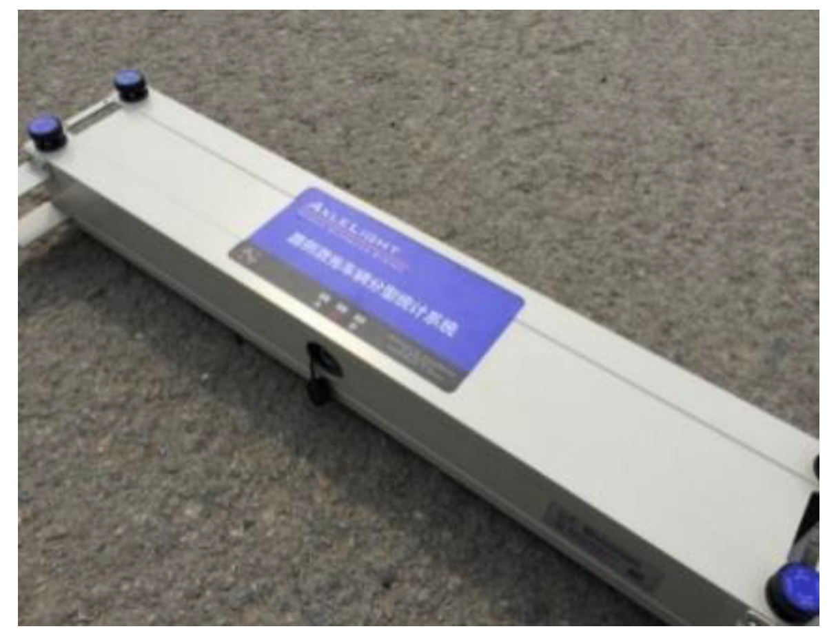
A real-time fuel-consumption monitoring instrument (Shenzhou JDSZ-EP-1-1D, Shanghai, China) was selected for this test, as presented in Figure 1. With the use of JDSZ EP-1-1D, second-by-second operating speed and fuel consumption were gathered during the trip on circular curves, and carbon emission data were calculated on the basis of the carbon emission conversion methodology.

2.2.2. Definition of Traffic Flow Pattern

The field test aims at investigating carbon emissions of the test vehicle on different circular curves. Additional emissions are generated if the test vehicle is disturbed by other vehicles during driving. Traffic flow conditions exert an impact on vehicle operating conditions and driver behavior [25,26]. In a comparatively congested traffic flow condition, vehicles have interference with each other, and individual vehicle velocity patterns are inclined to exhibiting fluctuating speeds. The number of acceleration and deceleration events of the vehicle increases, causing the additional fuel consumption and carbon emissions, correspondingly. The free-flow pattern is generally considered to be the vehicle driving merely impacted by the conditions of the road itself and is not interfered with by other vehicles [27]. Accordingly, it is deemed essential to clearly define the pattern of traffic flow during the test.

Traffic flow patterns are typically categorized by the service level [28]. The “Technical Standard of Highway Engineering” stipulated that v/C was an indicator for the evaluation of the road service level, as presented in

Table 1. Road service level details of Expressway.

The Degree of Road Service Level	v/C	Design Speed (km/h)
		120	100	80
		Maximum Traffic [pcu/(h·ln)]	Maximum Traffic [pcu/(h·ln)]	Maximum Traffic [pcu/(h·ln)]
1	v/C ≤ 0.35	750	730	700
2	0.35 < v/C ≤ 0.55	1200	1150	1100
3	0.55 < v/C ≤ 0.75	1650	1600	1500
4	0.75 < v/C ≤ 0.9	1980	1850	1800
5	0.90 < v/C ≤ 1.0	2200	2100	2000
6	v/C > 1.0	0~2200	0~2100	0~2000

Note: v/C is the ratio of the maximum service traffic volume to the basic traffic capacity. The basic traffic capacity is the maximum hourly traffic volume corresponding to level-of-service 5.

and

Table 2. Road service level details of First-class road.

The Degree of Road Service Level	v/C	Design Speed (km/h)
		100	80	60
		Maximum Traffic [pcu/(h·ln)]	Maximum Traffic [pcu/(h·ln)]	Maximum Traffic [pcu/(h·ln)]
1	v/C ≤ 0.3	600	550	480
2	0.3 < v/C ≤ 0.5	1000	900	800
3	0.5 < v/C ≤ 0.7	1400	1250	1100
4	0.7 < v/C ≤ 0.9	1800	1600	1450
5	0.9 < v/C ≤ 1.0	2000	1800	1600
6	v/C > 1.0	0~2000	0~1800	0~1600

Note: v/C is the ratio of the maximum service traffic volume to the basic traffic capacity. The basic traffic capacity is the maximum hourly traffic volume corresponding to level-of-service 5.

. There were several different service levels, represented by numbers 1 (least congested) to 6 (most congested) [27], correspondingly representing the level of the road congestion it provides for travelers. It also shed light on the fact that when the expressway and the first-class road are at level-of-service 1, the traffic flow is in a free-flow pattern.

Level-of-service 1 corresponds to the free-flow pattern. At this time, vehicles do not interfere with each other; the driver is able to drive freely, the driving speed is high, and the acceleration and deceleration options are comparatively more random. The free-flow pattern of a vehicle generally refers to a vehicle whose speed is merely impacted by its own road conditions, and the speed is not associated with other accompanying vehicles.

The definition of traffic flow pattern during field trials was asked to be the free-flow pattern, with no other accompanying vehicles driving on overtaking lanes and emergency parking lanes. Drivers were asked to operate trucks in the free flow pattern for the purpose of eliminating a situation that could be interfered with by other vehicles. The vehicle classification statistical system was employed for the measurement of the traffic volume during the test, as presented in Figure 2, which was realized by laser measurement technology.

2.2.3. Driver Selection

Owing to the fact that the driver’s performance varies depending on personal driving characteristics, it is deemed essential to select the drivers prior to the commencement of the field test. The drivers were required to be familiar with test roads and have a rich driving experience. Additionally, 10 days of training and testing was prepared for drivers, aimed at avoiding the impact of improper driving operations on test results. The drivers were asked to drive normally, meanwhile disallowing aggressive driving behavior, maintaining a safe distance from the preceding vehicle. There were 5 male drivers with driving experience between 10 and 15 years, having passed the training and exam.

2.2.4. Route Selection

The “Design Specification for Highway Alignment” [29] stipulated that the roadway gradient of the expressway should not be below 0.3%; accordingly, the test is carried out under a small roadway gradient range (−1%~−0.3% or 0.3%~1%), leading to the field test not being carried out on a completely flat road.

In accordance with "Design Specification for Highway Alignment", the minimum circular curve radius corresponded to the design speed of 60 km/h is 200 m. Furthermore, the associated research [30] dealing with the operating speed put forward that when the radius is greater than 500 m, the circular curve has less impact on the operating speed. It can be tentatively put forward that a circular curve, having a radius greater than 500 m, insignificantly impacts carbon emissions. As a consequence, the maximum circular curve radius in this study was tentatively set at 500 m, requiring verification by means of the following analysis.

Four highways in western China were selected as test sites. The road type was the key arterial road that had a design speed greater than, or equal to, 60 km/h, besides being without roundabouts and crossings. Unquestionably, there were two two-lane National Expressways, namely, Xianyang to Xunyi Expressway, and Xi’an to Hanzhong Expressway. Moreover, there were two provincial roads: Tawan to Jingbian road and Zhiwangchuan to Matouguan road. The radius of circular curves increased from 200 m to 550 m with a maximum increase of 50 m. The gradient of the test road was −1% to 0.3% or 0.3% to 1%. In total, 23 circular curve sections were selected and tested. The entering velocity of the vehicle increased from 60 km/h to 100 km/h with a maximum increase of 10 km/h.

A flat line section (length 2 km, gradient 0.3%) was selected on Xibao Expressway. The drivers were required to drive at a constant speed (from 60 to 100 km/h with a mean increase of 10 km/h) for the purpose of obtaining fuel consumption.

2.2.5. Other Factors

Since the current research work aimed at investigating the association between circular curve design features and carbon emissions, numerous measures were taken for the avoidance of the effect from other factors. In the field test, carbon emissions of the test vehicle on circular curves were carried out under a controlled condition, wherein the curve radius was changed, while other factors, for instance, the vehicle load, skills of the driver, vehicle age distribution, and climate conditions, remained fixed. The detailed conditions in the field test have been presented in

Table 3. Basic conditions in field test.

Variable	Specification
Vehicle Type	heavy truck ( type CA5310CCYP66K2L7T4E5, Jiefang, Jilin, China)
Vehicle Mass (t)	30
Heavy truck age	3 years
Fuel	Conventional diesel fuel, type is 10#
Driving age	10–15 years
Data	2 December 2017, to 5 January 2018, 9:00 am to 1 pm on weekdays
Temperature (°C)	−3~−5
Relative humidity (%)	75~85

.

3. Results

3.1. Field Test Data

There were 99 groups test data on 23 circular curve sections that satisfied the test requirements, as presented in

Table 4. Partial Data of field test on different curve radius.

No.	R (m)	L(m)	V0 (km/h)	FC (mL)	CE(g)
1	200	242.141	60.21	79	206
2	245	301.099	61.24	92	240
3	260	295.055	62.98	86	225
4	285	370.801	61.45	104	270
5	300	296.470	62.68	82	213
…	…	…	…	…	…
95	600	651.348	100.13	267	695
96	700	640.806	100.22	262	681
97	800	935.096	102.2	384	999
98	900	868.356	101.21	356	926
99	1000	1251.348	103.49	511	1330

. Velocity and fuel consumption were gathered from a field test, followed by calculating carbon emissions with the help of the carbon emission conversion methodology. With regard to the tests on each circular curve with different entering velocity, the following data were obtained: radius (R), circular curve length (L), entering velocity (V₀), fuel consumption (FC), and carbon emissions (CE).

CEP (g/m) was defined as the carbon emission rate of vehicles all through the trip, and FCP (g/m) was defined as the fuel consumption rate of vehicles all through the trip, as presented in Equations (6) and (7).

CEP = CE/L,

(6)

FCP = FC/L,

(7)

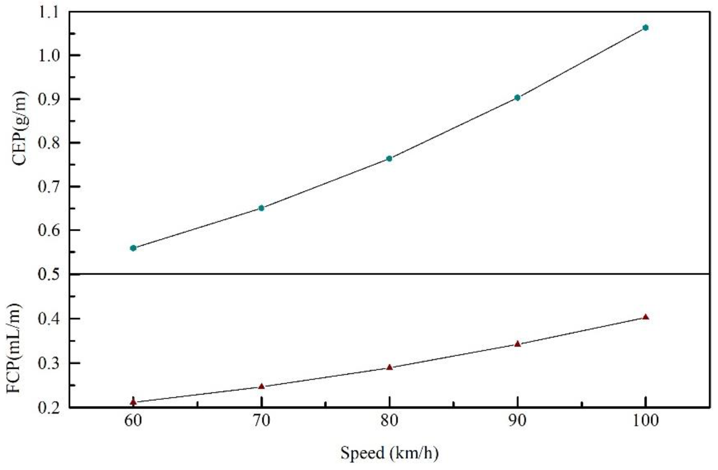
The relevant data of the heavy truck collected on flat line sections are presented in Figure 3.

Figure 3 sheds light on the amount of fuel consumption and carbon emissions of the heavy truck with different uniform speed on a flat line. The higher speed accompanied the higher vehicle specific power and engine load [31,32]. With the increase in the engine load, fuel and carbon emission output responds faster. Figure 3 reveals that fuel consumption and carbon emissions increase linearly or exponentially with speed within a specific range.

Figure 4 sheds light on the carbon emissions of a heavy truck with different entering speeds on circular curves. In comparison with the circular curve having a large radius, the carbon emissions of a heavy truck on a circular curve with a small radius are presented to be higher, accordingly giving rise to greater damage to the environment. Figure 4 sheds light on the fact that the carbon emissions decreased linearly or exponentially with their radius ranging between 200 m and 550 m. With the radius exceeding 550 m, there were almost no significant CO₂ data difference, and the carbon emissions were close to the carbon emissions on the flat line section. Accordingly, the radius of the curve in the carbon emission model was defined to be ranging between 200 m and 550 m, and there were 74 groups of test data for the establishment of the carbon emission prediction model on a circular curve. Figure 4 suggests that analysis is required for the purpose of attaining the minimum curve radius when vehicle carbon emissions attained on both circular curves and flat lines are approximately equal. Details regarding this concern have been discussed in Section 3.3.

3.2. Carbon Emission Prediction Model

The data from the field test were employed for analyzing the carbon emission rule of the heavy truck on the circular curve. One-way ANOVA was carried out on carbon emission data with the use of SPSS, wherein the curve radius R, length of circular curve L, and entering velocity V₀ were independent variables, whereas CPE was the dependent variable. The significance level was defined as 0.05. Subsequent to that, the optimal regression models for f (R), f (L), and f (V₀) were correspondingly attained, in accordance with the BIC (Bayesian Information Criterion). BIC places emphasis on the superiority of data fitting, meanwhile focusing more on avoiding overfitting, which is generally put to use for the evaluation of whether the model possesses the highest simplicity and precision. A smaller BIC value suggests a greater fit precision and conciseness of the regression model.

Analysis of the relationship between curve radius R and CPE was taken into consideration as an example. The linear, quadratic, and cubic regression models were fitted correspondingly in accordance with the field test data. The significance probability (P) of quadratic regression model was 0.001 < 0.05, which revealed the confidence interval to be higher than 95%. Besides, the quadratic regression model had a higher R² value of 0.753, together with a higher F value of 539.017 as compared with other regression models, as presented in Table 3. The parameters suggested that the quadratic regression model fitted well with the data set requirements, in addition to offering a higher precision. The BIC value of the quadratic model was smaller than other models, which suggested that there was no over-fitting in the quadratic model. Accordingly, the optimal regression model for CEP and circular curve radius was f (R)₂. Three optimal unary regression models (f (R)₂, f (L)₃, and f (V₀)₂) were separately attained by means of the same approach, as listed in

Table 5. Numerical summary of different unary regressions.

Independent Variables	Unary Regression Model	One-Way ANOVA			BIC	Optimal Model
		R2	F	P
R	f (R)1 = 0.823 − 0.001R	0.602	514.953	0.003	320.478	f (R)2
	f (R)2 =0.913 − 0.001R + 6.748 × 10−7R2	0.753	539.017	0.001	176.924
	f (R)3 = 0.147 − 0.006R − 1.756e−5R2 + 1.610 e−8R3	0.628	522.452	0.003	298.969
L	f (L)1 = − 0.110ln(L) + 0.907	0.649	314.977	0.001	403.905	f (L)3
	f (L)2 = 0.950 − 0.001 L + 7.538e−7L2	0.628	300.751	0.020	462.067
	f (L)3 = 1.507 L−0.223	0.687	533.781	0.001	251.620
V0	f (V0)1 = 0.627 + 0.004V0	0.565	963.273	0.022	172.714	f (V0)2
	f (V0)2 = 1.193 − 0.010V0 + 8.571e−5V02	0.689	517.542	0.011	155.439

. These models had a significance level P < 0.05, together with higher F and R² test values, and BIC value was smaller than other models, which suggested that these models offered the highest precision and simplicity. Together, it also sheds light on the fact that all variables (R, L and V₀) had pivotal impacts on the carbon emission rate.

On the basis of the optimal models, a nonlinear multiple regression model was established, wherein a required significance level of 0.05 was defined; moreover, the R, R², Lⁿ, V₀, and V₀² were taken as explanatory variables, and CEP was put to use as the dependent variable. The descriptive statistics results revealed the fact that the R² value was 0.917, which implied that the model had a good interpretation ability. On the basis of the results of the iterative nonlinear multiple regression analysis, the carbon emission prediction model of a heavy truck on a circular curve can be attained, which is expressed as Equation (8)

CE = L × CEP,                               
= L × (1.28 − 0.0029R + 2.738 × 10⁻⁶R² − 0.0022 × L^−0.223 − 0.00617V₀ + 0.000117 V₀²),

(8)

R ∈ (200 m, 550 m), Roadway gradient ∈ (−1%, −0.3%), (0.3%, 1%)

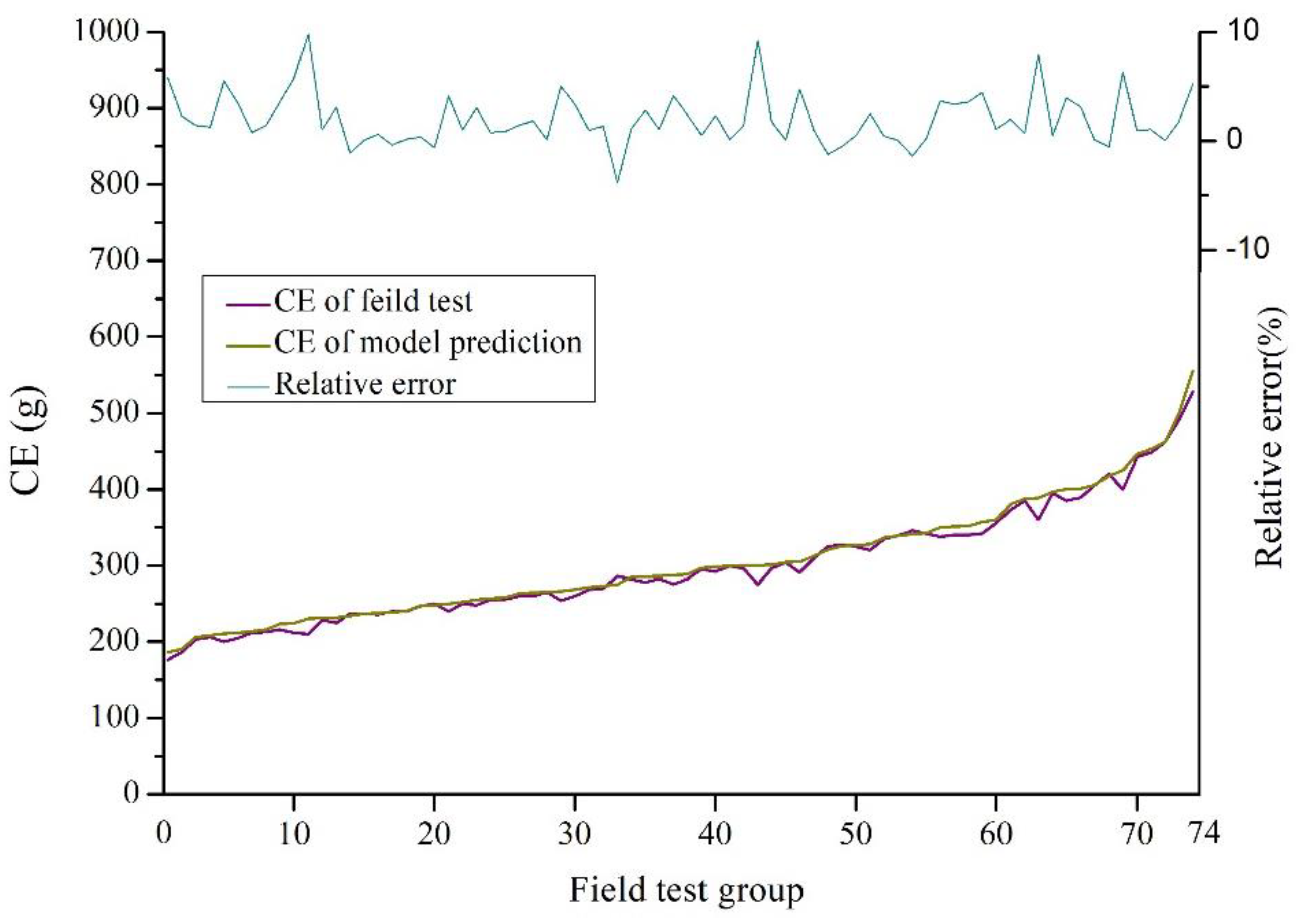
The predicted values of the model were compared with 74 groups of measured data in Figure 5. The order of the field test was reordered on the basis of carbon emission prediction values for the clear demonstration of the prediction ability of the model. The relative error of the carbon emission prediction model is below 10%, which suggested that the accuracy met the requirements.

3.3. The Minimum Curve Radius Affecting Carbon Emissions

The carbon emissions of heavy trucks on a large radius circular curve are presented to be close to the carbon emissions on the flat line. It is deemed essential to figure out the radius value, while vehicle carbon emissions on the circular curve and the flat line are approximately equal. The radius attained is the minimum radius impacting vehicle carbon emissions.

The field test is incapable of attaining initial velocity to a specific value, and the radius value cannot be changed with a regular difference. It is quite tough to analyze directly with the help of the field test data. Taking into consideration the high accuracy of the prediction model, the following analysis made use of the carbon emission data predicted by the prediction model. All through the prediction, the vehicle carbon emissions under different scenarios for which the trip was designed 100 m, curve radius increased from 200 m to 550 m with a mean increase of 50 m, and entering velocity increased from 60 km/h to 100 km/h with a mean increase of 10 km/h. Carbon emission data measured on a flat line in a field test was converted to the data for a 100 m trip. The carbon emission data predicted under different circular curves scenarios were compared with the carbon emission data measured on the flat line in the field test, as presented in

Table 6. Partial carbon emissions comparison on circular curve and flat line.

Speed (km/h)	The Radius of Circular Curve								Flat Line
	200	250	300	350	400	450	500	550
60	86.035	77.696	70.725	65.124	60.891	58.028	56.533	56.408	55.910
70	95.075	86.736	79.765	74.164	69.931	67.068	65.573	65.448	65.024
80	106.455	98.116	91.145	85.544	81.311	78.448	76.953	76.828	76.383
90	120.175	111.836	104.865	99.264	95.031	92.168	90.673	90.548	90.307
100	136.235	127.896	120.925	115.324	111.091	108.228	106.733	106.608	106.312

.

Table 6 sheds light on the fact that the larger the curve radius, the lower the carbon emissions generated from the vehicle with the same entering velocity. With the increase in the radius, carbon emissions gradually decrease. Overall, a circular curve section with a large radius and flat line section allows vehicles to reach a higher speed in a short time, together with maintaining the speed with a smaller acceleration value, which leads to lower carbon emissions.

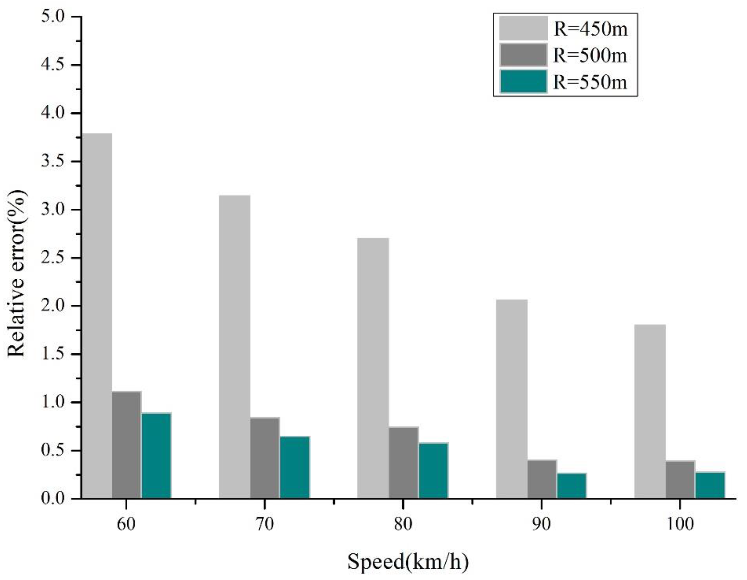
As evident from Table 6, the carbon emissions predicted in the scenarios with a circular curve radius of 550 m is close to the carbon emissions attained on the flat line. On the basis of the simulation results, the relative error values of carbon emissions between curves radius and flat line scenarios have been presented in

Table 7. Relative error of carbon emissions in simulated scenarios.

Speed (km/h)	The Radius of Circular Curve
	200	250	300	350	400	450	500	550
60	53.881	38.966	26.498	16.479	8.909	3.788	1.115	0.890
70	46.215	33.390	22.670	14.056	7.547	3.143	0.844	0.651
80	39.370	28.452	19.326	11.993	6.452	2.703	0.746	0.582
90	33.074	23.839	16.121	9.918	5.231	2.060	0.405	0.266
100	28.147	20.302	13.746	8.477	4.495	1.802	0.396	0.278

. With regard to the scenarios with a radius of 450 m, 500 m, and 550 m, the relative errors of carbon emissions with a flat line scenario were comparatively smaller. When a heavy truck was driving on the circular curve with radius of 550 m, coupled with the entering speed of 60 km/h, the carbon emissions value is close to the carbon emissions on the flat line with a uniform speed of 60 km/h, and the relative error is 0.89%. In the same manner, the relative error attained between the scenarios on a radius of 450 m and a flat line with a speed of 60 km/h is 3.788%.

With regard to the radius of 450 m scenarios in Figure 6, there is a comparatively larger increase in the relative error of carbon emissions in comparison with the radius of 500 m and 550 m scenarios. Figure 6 sheds light on the fact that the relative error of carbon emissions between circular curve R = 500 m scenarios and flat line scenarios is comparatively smaller, besides being merely second to the radius of 550 m scenarios. The vehicle carbon emissions under the radius of 500 m and 550 m scenarios are quite close, and the relative errors at the radius of 500 m scenarios are less than 5%. Taking into consideration the above analysis findings, as well as the relative error of prediction model, the minimum circular curve radius R = 500 m impacting the carbon emissions can be attained, which is in line with the assumption mentioned earlier. It reveals the fact that the test vehicle not only consumed more fuel but also produced more carbon emissions on circular curves with below-minimum radius scenarios.

4. Discussion

In the current paper, a carbon emission model for the quantification of vehicle carbon emissions on circular curves was established, and the minimum radius of circular curves impacting carbon emissions was attained.

For the purpose of obtaining the relationship between tailpipe CO₂ emissions and fuel consumption subjected to the present status of diesel in China, the associated data of diesel combustion at current diesel status in China were matched with the help of the IPCC’s carbon emission calculation methodology. Through the analysis of the data obtained from the field test, a carbon emission model for the heavy truck on different circular curves was established. The prediction model can be put to use during the highway horizontal alignment design and operational stage to quantify the adverse environmental impacts from vehicle movements. Besides that, through the comparison of the carbon emission data attained from the prediction model with the carbon emission data attained from the field test, it is evident that the carbon emission prediction model has a comparatively lower relative error, in addition to high accuracy and credibility. The model can also be applied to the vehicle fuel consumption prediction, based on the robust relationship between fuel consumption and tailpipe CO₂ emissions.

The minimum radius of a circular curve impacting the vehicle carbon emissions is 500 m. This conclusion is reached through the comparison of the vehicle carbon emissions on a circular curve section and flat line section. The research work, which considers the association between highway design and carbon emissions, can be combined with the findings of the current study for the purpose of ultimately enhancing the environmental highway design.

Owing to the fact that a heavy truck was selected as a test vehicle for the field test, followed by establishing a carbon emission model, the model is incapable of quantifying the carbon emissions of other vehicles. Together with that fact, the traffic flow pattern during the field test was defined as a free-flow pattern and no other accompanying vehicles were driving in the overtaking lane and emergency parking lane, aimed at eliminating interference from other vehicles. It was shown that the model does not have the potential of fully reflecting the carbon emissions rule of the passing vehicles in different traffic flow patterns. That requires additional observation, while the current research work places emphasis only on the association between carbon emissions and circular curves. Nevertheless, the carbon emission prediction model of other types of vehicles can be investigated in subsequent studies on the basis of the carbon emission rule of the current study. Also, the prospective research, emphasizing the quantification of carbon emissions, requires consideration of the impacts of other factors (for instance, traffic flow conditions, vehicle load, and driving performance) on vehicle carbon emissions. Furthermore, the combined impacts of these factors under special situations require further investigation.

5. Conclusions

The present research work put forward a carbon emission conversion methodology based on the IPCC’s carbon emission calculation methodology through the addition of the characteristics of China’s diesel status. The conclusions of the current paper are comparable with the existing research results, both at home and abroad, and the applicability of carbon emission conversion methodology in China is guaranteed.

The carbon emission prediction model established in this research can be employed for the quantification of the vehicle carbon emissions on circular curves, providing supporting data for the comparison of route schemes for low-carbon design. The result of the minimum circular curve radius impacting the carbon emissions has the potential to provide the basis for the low-carbon design of highway circular curves.

References

1. Harrington, W.; Mcconnell, V.D.; Cannon, M. A Behavioral Analysis of EPA’s MOBILE Emission Factor Model; Discussion Papers No 98-47; Resources for the Future: Washington, DC, USA, 1998. [Google Scholar]
2. Huang, Y.; Hakim, B.; Zammataro, S. Measuring the carbon footprint of road construction using CHANGER. Int. J. Pavement Eng. 2013, 14, 11. [Google Scholar] [CrossRef]
3. Zhai, H.; Frey, H.C.; Rouphail, N.M. Comparison of Flexible Fuel Vehicle and Life-Cycle Fuel Consumption and Emissions of Selected Pollutants and Greenhouse Gases for Ethanol 85 Versus Gasoline. J. Air Waste Manag. Assoc. 2009, 59, 912–924. [Google Scholar] [CrossRef] [PubMed] [Green Version]
4. Guo, H.; Zhang, Q.Y.; Shi, Y. Evaluation of the International Vehicle Emission (IVE) model with on-road remote sensing measurements. J. Environ. Sci. 2007, 19, 818–826. [Google Scholar] [CrossRef]
5. Abou-Senna, H.; Radwan, E.; Westerlund, K. Using a traffic simulation model (VISSIM) with an emissions model (MOVES) to predict emissions from vehicles on a limited-access highway. J. Air Waste Manag. Assoc. 2013, 63, 819–831. [Google Scholar] [CrossRef] [PubMed] [Green Version]
6. Jiao, S.; Hou, C.; Li, Y.; Du, Q. Establishing the CO2 emission model of carbon neutral road based on gradient. Electrical and Control Engineering (ICECE). In Proceedings of the 2011 International Conference on Electrical and Control Engineering, Yichang, China, 16–18 September 2011; pp. 4494–4497. [Google Scholar]
7. Sobrino, N.; Monzon, A. Towards Low-Carbon Interurban Road Strategies: Identifying Hot Spots Road Corridors in Spain. Sustainability 2018, 10, 3963. [Google Scholar] [CrossRef]
8. Sobrino, N.; Monzon, A.; Hernández, S. Reduced Carbon and Energy Footprint in Highway Operations: The Highway Energy Assessment (HERA) Methodology. Netw. Spat. Econ. 2016, 16, 395–414. [Google Scholar] [CrossRef]
9. Yang, W.; Alessandra, B.M. Evaluation of Eco-Driving Training for Fuel Efficiency and Emissions Reduction According to Road Type. Sustainability 2018, 10, 3891. [Google Scholar]
10. Ko, M.; Lord, D.; Zietsman, J. Environmentally Conscious Highway Design for Crest Vertical Curves. Transp. Res. Rec. J. Transp. Res. Board 2012, 2270, 96–106. [Google Scholar] [CrossRef]
11. Jia, X.; Xu, J.; Liu, X. Association of Carbon emissions and Expressway Longitudinal Slope in Northern China. J. Residuals Sci. Technol. 2017, 14, 177–183. [Google Scholar] [CrossRef]
12. Ko, M. Incorporating Vehicle Emissions Models into the Geometric Highway Design Process: Application on Horizontal Curves. In Proceedings of the Transportation Research Board 94th Annual Meeting, Washington, DC, USA, 11 January 2015. [Google Scholar]
13. David, L.; Ana María, P.; Alfredo, G. Impact of horizontal geometric design of two-lane rural roads on vehicle CO2 emissions. Transp. Res. Part D Transp. Environ. 2018, 59, 46–57. [Google Scholar]
14. Barth, M.; K, B. Real-World Carbon Dioxide Impacts of Traffic Congestion. In Transportation Research Record: Journal of the Transportation Research Board; No. 2058; Transportation Research Board of the National Academies: Washington, DC, USA, 2010; pp. 163–171. [Google Scholar]
15. Jiao, S.; Li, L.; Li, Y. Research on Design Index of Low-Carbon Highway Route Based on Game Theory. Adv. Mater. Res. 2013, 869, 1039–1043. [Google Scholar] [CrossRef]
16. Bonneson, J.; Pratt, M. Model for Predicting Speed Along Horizontal Curves on Two-Lane Highways. Transp. Res. Rec. J. Transp. Res. Board 2009, 2092, 19–27. [Google Scholar] [CrossRef]
17. Kang, M.; Shariat, S.; Jha, M. New highway geometric design methods for minimizing vehicular fuel consumption and improving safety. Transp. Res. Part C Emerg. Technol. 2013, 31, 99–111. [Google Scholar] [CrossRef]
18. Hu, W.; Donnell, E.T. Models of acceleration and deceleration rates on a complex two-lane rural highway: Results from a nighttime driving experiment. Transp. Res. Part F Traffic Psychol. Behav. 2010, 13, 397–408. [Google Scholar] [CrossRef]
19. May, J.; Favre, C. On-Road Testing and PEMS Data Analysis for two Euro 6 Diesel Vehicles. SAE Int. J. Fuels Lubr. 2014, 7, 919–934. [Google Scholar]
20. Mamakos, A.; Bonnel, P.; Perujo, A. Assessment of portable emission measurement systems (PEMS) for heavy-duty diesel engines with respect to particulate matter. J. Aerosol Sci. 2013, 57, 54–70. [Google Scholar] [CrossRef]
21. IPCC (Intergovernmental Panel on Climate Change). Guidelines for National Greenhouse Gas Inventories; Egglestone, H.S., Buendia, L., Miwa, K., Ngara, T., Tanabe, K., Eds.; Volume 2: Energy; Prepared by the National Greenhouse Gas Inventories Program; IGES: Tsukuba, Japan, 2006. [Google Scholar]
22. National Development and Reform Commission, Climate Change Division. In Second National Communications on Climate Change in the People’s Republic of China; China Economic Publishing House: Beijing, China, 2013.
23. Chinese Government. The First Two-Year Update Report on Climate Change in the People’s Republic of China. Available online: http://www.webcitation.org/75mAIC7ah (accessed on 28 January 2019).
24. National Development and Reform Commission, Department of Climate Change, etc. Guidelines for the Preparation of Provincial Greenhouse Gas Inventories (Trial); NDRC: Beijing China, 2011.
25. Arti, C.; Sharad, G. Urban real-world driving traffic emissions during interruption and congestion. Transp. Res. Part D 2016, 43, 59–70. [Google Scholar]
26. Yang, S.; Ji, Y.; Zhang, D. Equilibrium between Road Traffic Congestion and Low-Carbon Economy: A Case Study from Beijing, China. Sustainability 2019, 11, 219. [Google Scholar] [CrossRef]
27. Technical Standards for Highway Engineering (JTG B01-2014); China Standard Press: Beijing, China, 2014.
28. Transportation Research Board (TRB). Highway Capacity Manual; Special Report 87; National Research Council: Washington, DC, USA, 2000. [Google Scholar]
29. Design Specification for Highway Alignment (JTG D20-2017); China Standard Press: Beijing, China, 2017.
30. Echaveguren, T.; Bustos, M.; de Solminihac, H. Assessment of horizontal curves of an existing road using reliability concepts. Can. J. Civ. Eng. 2005, 32, 1030–1038. [Google Scholar] [CrossRef]
31. Song, G.; Yu, L. Estimation of Fuel Efficiency of Road Traffic by Characterization of Vehicle-Specific Power and Speed Based on Floating Car Data. Transp. Res. Rec. J. Transp. Res. Board 2009, 2139, 11–20. [Google Scholar] [CrossRef]
32. Zhai, H.; Frey, H.C.; Rouphail, N.M. A Vehicle-Specific Power Approach to Speed- and Facility-Specific Emissions Estimates for Diesel Transit Buses. Environ. Sci. Technol. 2008, 42, 7985–7991. [Google Scholar] [CrossRef] [PubMed]
Figure 1. Fuel-consumption instrument used in field experiments.
Sustainability 11 01156 g001
Figure 2. Vehicle classification statistical system.
Sustainability 11 01156 g002
Figure 3. Data of field test on flat line.
Sustainability 11 01156 g003
Figure 4. The carbon emission rate of field test on circular curves.
Sustainability 11 01156 g004
Figure 5. Comparison of predicted and experimental results for carbon emissions.
Sustainability 11 01156 g005
Figure 6. Partial relative error of carbon emissions in simulated scenarios.
Sustainability 11 01156 g006