Monitoring the Characteristics of the Bohai Sea Ice Using High-Resolution Geostationary Ocean Color Imager (GOCI) Data


Abstract
1. Introduction
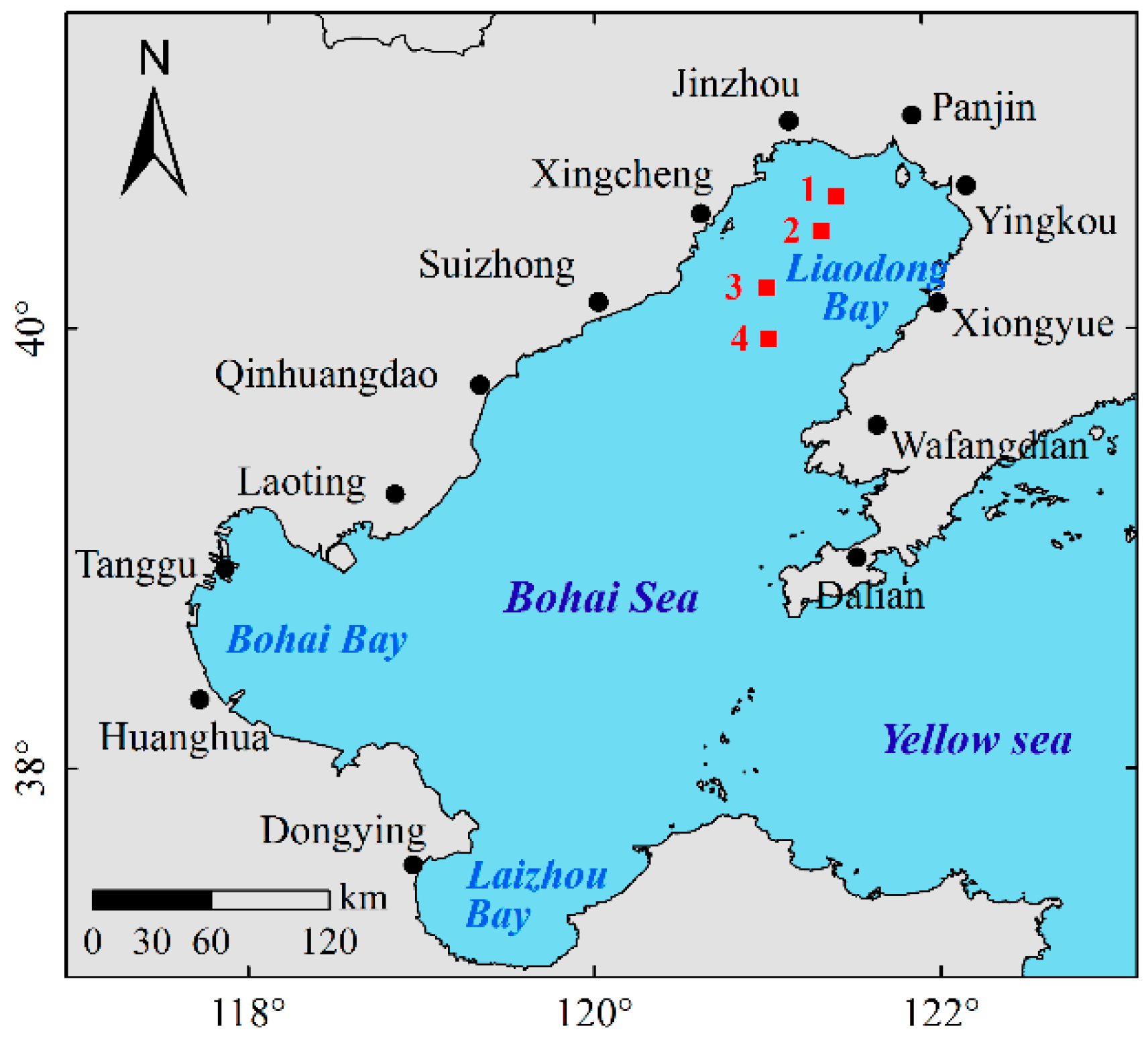
2. Study Area
3. Data and Methods
3.1. Data Description
3.1.1. Remote Sensing Data
3.1.2. Meteorological Data
3.1.3. In Situ Measurement of Sea Ice Thickness
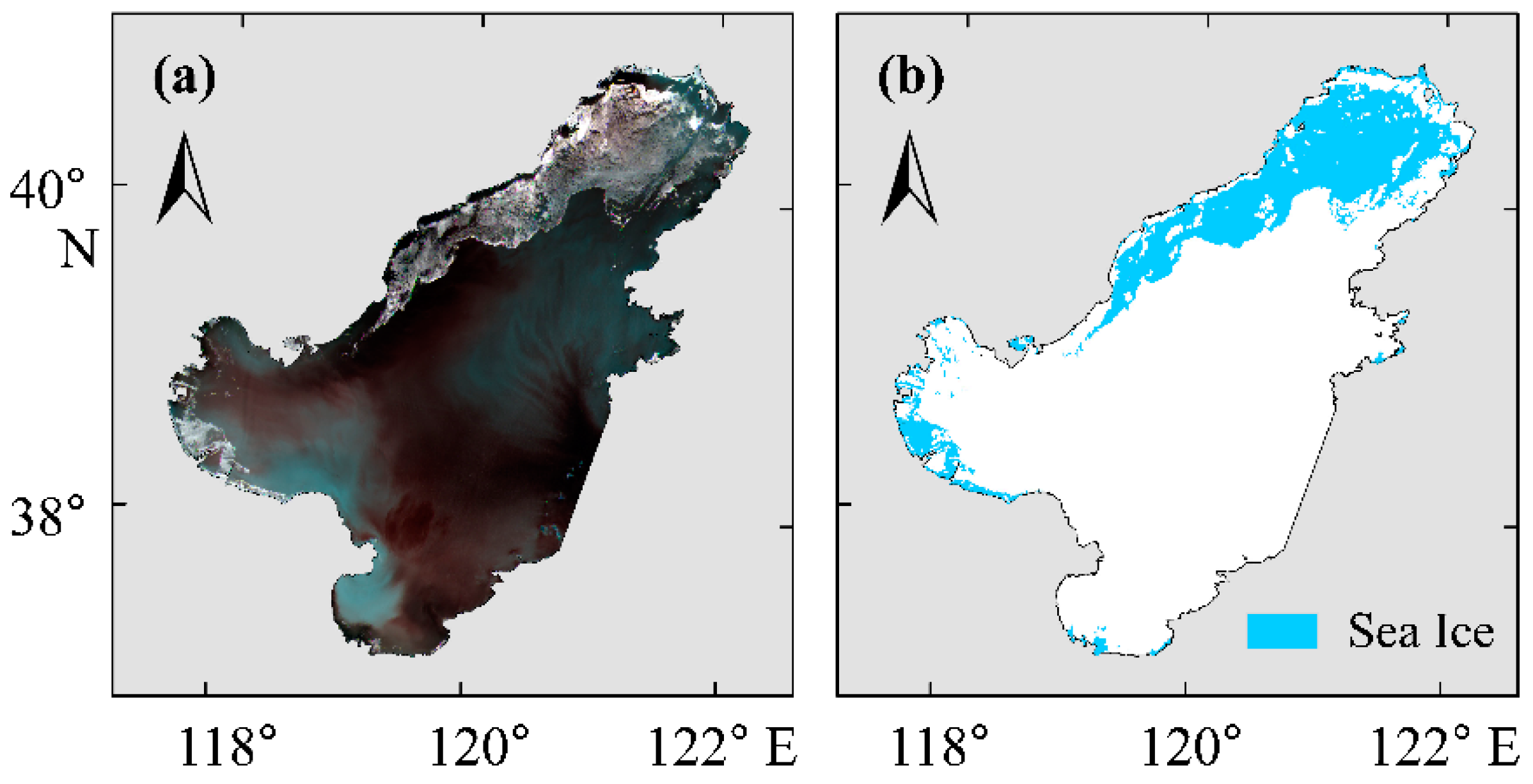
3.2. GOCI Data Pre-Processing
3.3. Extraction of Sea Ice Area
3.4. Sea Ice Thickness Inversion
+ 0.6204α6 − 0.1474α7 − 0.0268α8 − 0.0464,
3.5. Meteorological Parameters
4. Results
4.1. Sea Ice Area
4.1.1. Validation
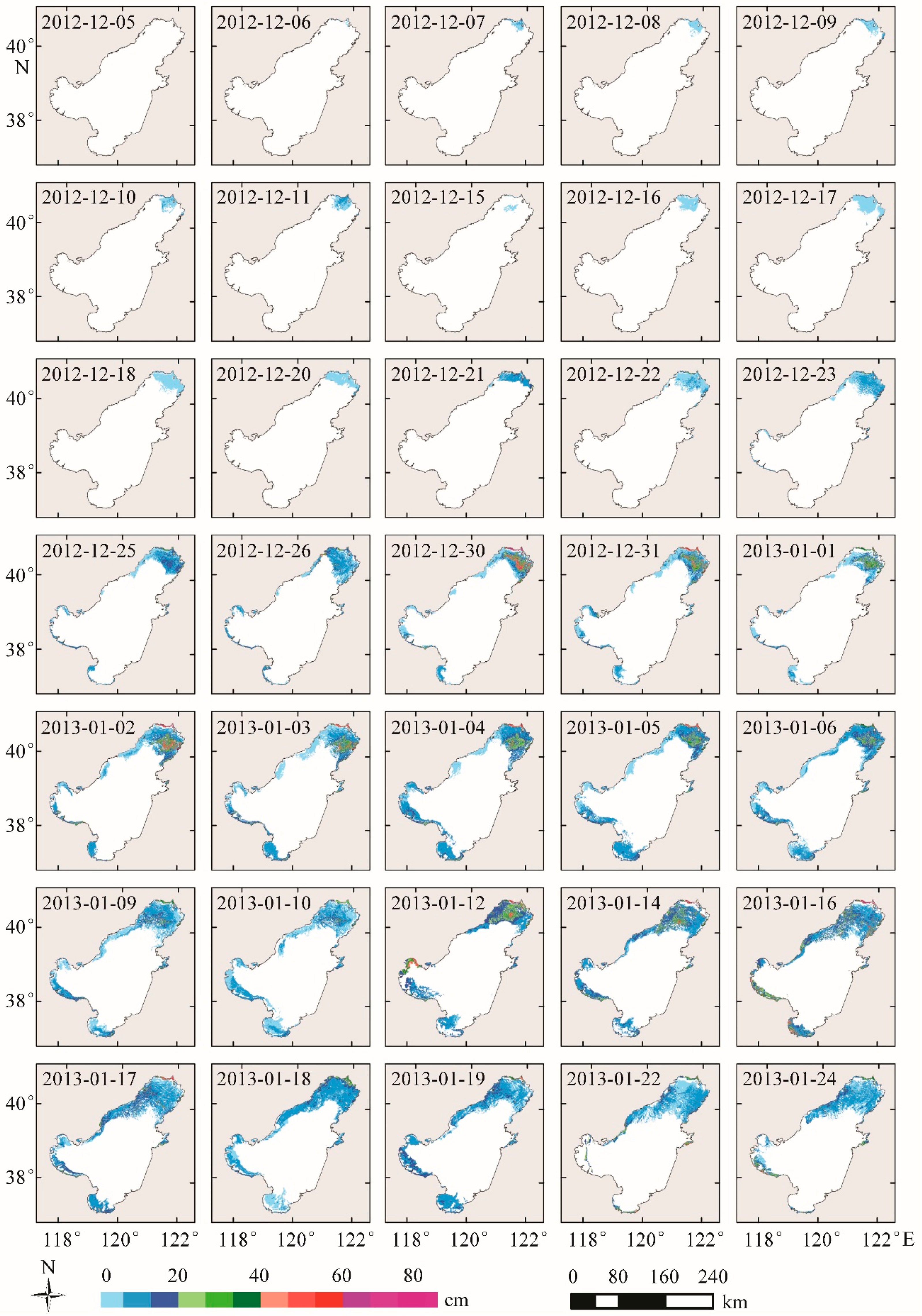
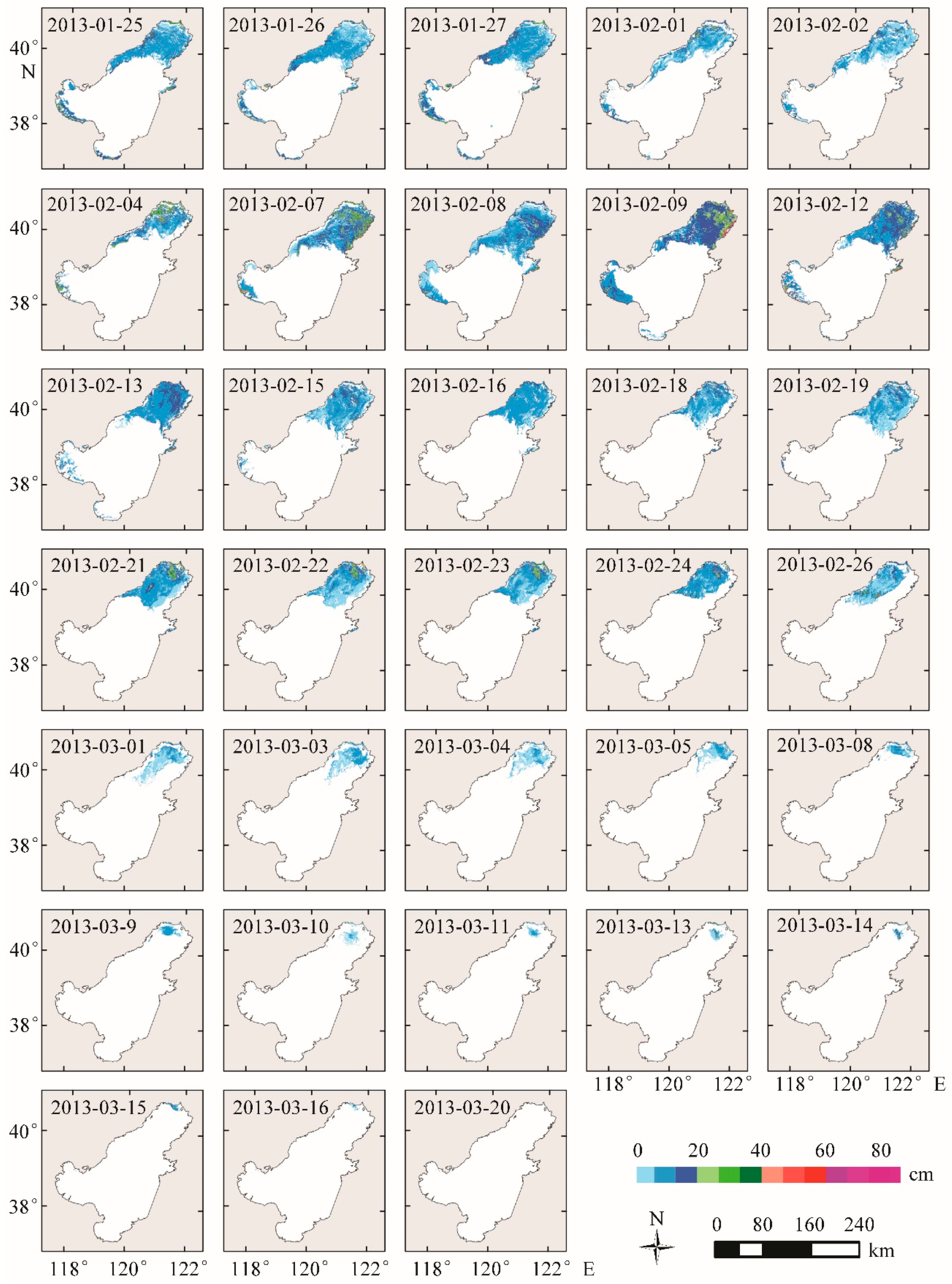
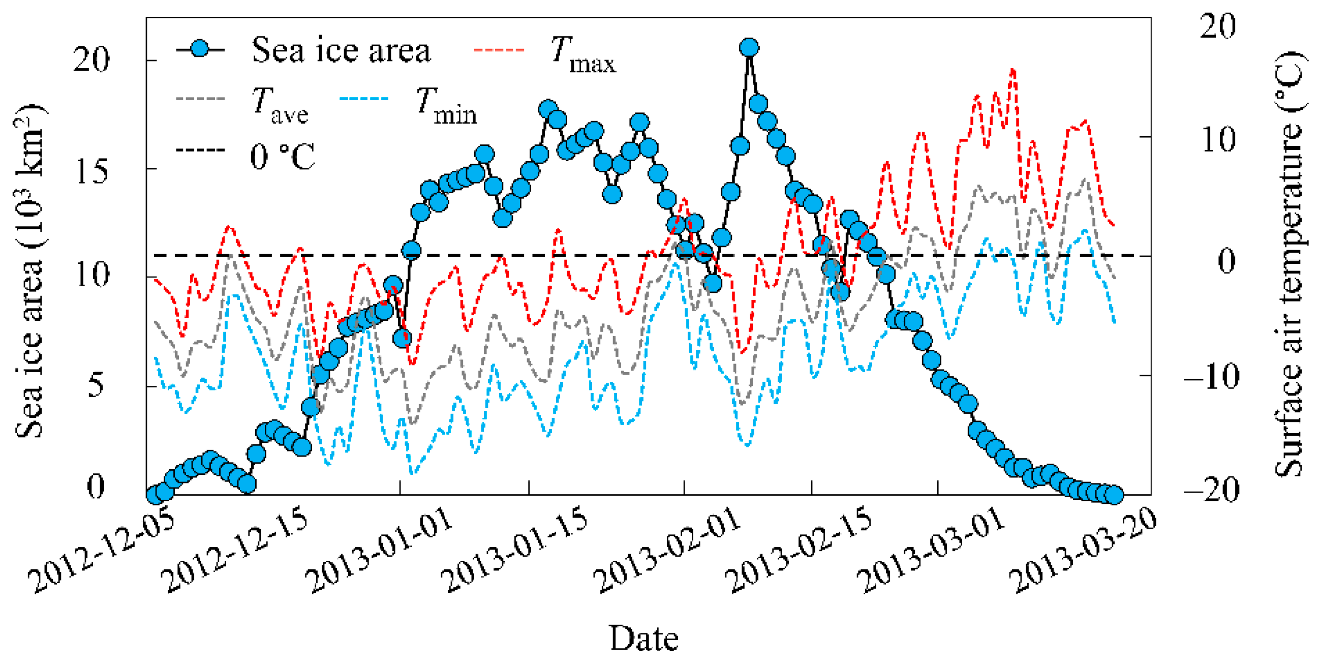
4.1.2. Spatiotemporal Distribution and Evolution
4.2. Sea Ice Thickness
4.2.1. Validation
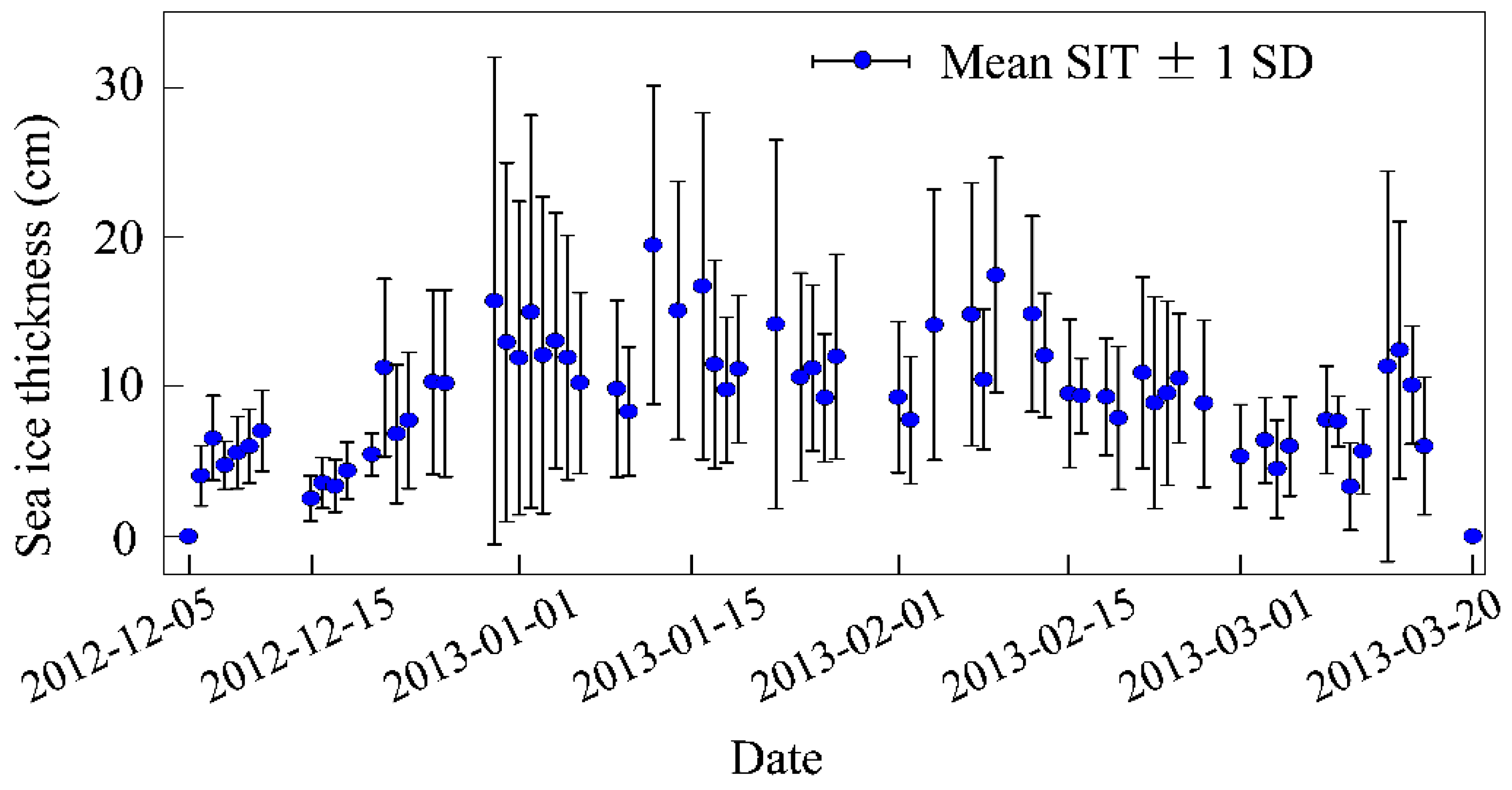
4.2.2. Spatiotemporal Distribution and Evolution
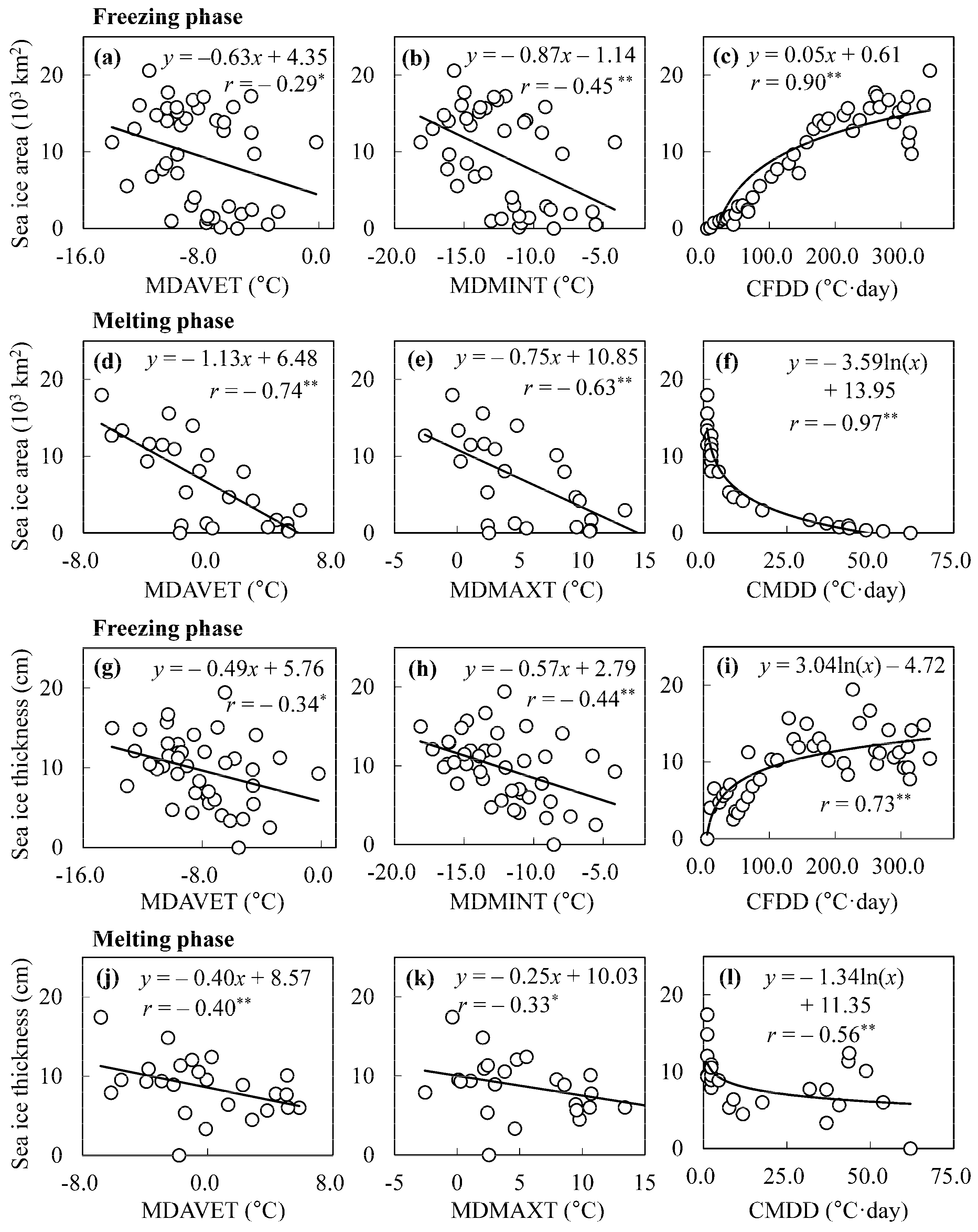
4.3. Correlations Between Sea Ice Characteristics and Meteorological Factors
5. Discussion
6. Conclusions
Author Contributions
Funding
Acknowledgments
Conflicts of Interest
References
- Gu, W.; Liu, C.Y.; Yuan, S.; Li, N.; Chao, J.L.; Li, L.T.; Xu, Y.J. Spatial distribution characteristics of sea-ice-hazard risk in Bohai, China. Ann. Glaciol. 2013, 54, 73–79. [Google Scholar] [CrossRef]
- Gong, D.Y.; Kim, S.J.; Ho, C.H. Arctic Oscillation and ice severity in the Bohai Sea, East Asia. Int. J. Climatol. 2007, 27, 1287–1302. [Google Scholar] [CrossRef]
- Bai, X.Z.; Wang, J.; Liu, Q.Z.; Wang, D.X.; Liu, Y. Severe ice conditions in the Bohai Sea, China, and mild ice conditions in the great lakes during the 2009/10 winter: Links to El Nino and a strong negative arctic oscillation. J. Appl. Meteorol. Clim. 2011, 50, 1922–1935. [Google Scholar] [CrossRef]
- Simmonds, I. Comparing and contrasting the behaviour of Arctic and Antarctic sea ice over the 35-year period 1979–2013. Ann. Glaciol. 2015, 56, 18–28. [Google Scholar] [CrossRef]
- Yan, Y.; Shao, D.; Gu, W.; Liu, C.Y.; Li, Q.; Chao, J.L.; Tao, J.; Xu, Y.J. Multidecadal anomalies of Bohai Sea ice cover and potential climate driving factors during 1988–2015. Environ. Res. Lett. 2017, 12, 094014. [Google Scholar] [CrossRef]
- Tao, S.S.; Dong, S.; Wang, Z.F.; Soares, C.G. Intensity division of the sea ice zones in China. Cold Reg. Sci. Technol. 2018, 151, 179–187. [Google Scholar] [CrossRef]
- Zhang, X.L.; Zhang, Z.H.; Xu, Z.J.; Li, G.; Sun, Q.; Hou, X.J. Sea ice disasters and their impacts since 2000 in Laizhou Bay of Bohai Sea, China. Nat. Hazards 2013, 65, 27–40. [Google Scholar] [CrossRef]
- Gu, W.; Lin, Y.B.; Xu, Y.J.; Yuan, S.; Tao, J.; Li, L.T.; Liu, C.Y. Sea ice desalination under the force of gravity in low temperature environments. Desalination 2012, 295, 11–15. [Google Scholar] [CrossRef]
- Liu, C.Y.; Gu, W.; Chao, J.L.; Li, L.T.; Yuan, S.; Xu, Y.J. Spatio-temporal characteristics of the sea-ice volume of the Bohai Sea, China, in winter 2009/10. Ann. Glaciol. 2013, 54, 97–104. [Google Scholar] [CrossRef]
- Tao, J.; Xu, Y.J.; Zhang, H.; Gu, W. The effect of brackish ice mulching on soil salinity content and crop emergence in man-made, raised bed on saline soils. Eurasian Soil Sci. 2018, 51, 658–663. [Google Scholar] [CrossRef]
- Xie, F.; Wei, G.U.; Yuan, Y.; Chen, Y.H. Estimation of sea ice resources in Liaodong gulf using remote sensing. Resour. Sci. 2003, 25, 17–23. (In Chinese) [Google Scholar]
- Ning, L.; Xie, F.; Gu, W.; Xu, Y.J.; Huang, S.Q.; Yuan, S.; Cui, W.J.; Levy, J. Using remote sensing to estimate sea ice thickness in the Bohai Sea, China based on ice type. Int. J. Remote Sens. 2009, 30, 4539–4552. [Google Scholar] [CrossRef]
- Shi, W.; Wang, M.H. Sea ice properties in the Bohai Sea measured by MODIS-Aqua: 2. Study of sea ice seasonal and interannual variability. J. Mar. Syst. 2012, 95, 41–49. [Google Scholar] [CrossRef]
- Su, H.; Wang, Y.P. Using MODIS data to estimate sea ice thickness in the Bohai Sea (China) in the 2009–2010 winter. J. Geophys. Res. 2012, 117, C10018. [Google Scholar] [CrossRef]
- Yuan, S.; Gu, W.; Xu, Y.J.; Wang, P.; Huang, S.Q.; Le, Z.Y.; Cong, J.O. The estimate of sea ice resources quantity in the Bohai Sea based on NOAA/AVHRR data. Acta Oceanol. Sin. 2012, 31, 33–40. [Google Scholar] [CrossRef]
- Yuan, S.; Liu, C.Y.; Liu, X.Q. Practical model of sea ice thickness of Bohai Sea based on MODIS data. Chin. Geogr. Sci. 2018, 28, 863–872. [Google Scholar] [CrossRef]
- Liu, C.; Chao, J.L.; Gu, W.; Xu, Y.J.; Xie, F. Estimation of sea ice thickness in the Bohai Sea using a combination of VIS/NIR and SAR images. GISci. Remote Sens. 2015, 52, 115–130. [Google Scholar] [CrossRef]
- Zhang, X.; Dierking, W.; Zhang, J.; Meng, J.M. A polarimetric decomposition method for ice in the Bohai Sea using C-band PolSAR data. IEEE J. Sel. Top. Appl. Earth Obs. Remote Sens. 2015, 8, 47–66. [Google Scholar] [CrossRef]
- Karvonen, J.; Shi, L.J.; Cheng, B.; Simila, M.; Makynen, M.; Vihma, T. Bohai Sea ice parameter estimation based on thermodynamic ice model and Earth observation data. Remote Sens. 2017, 9, 234. [Google Scholar] [CrossRef]
- Dierking, W. Sea ice monitoring by synthetic aperture radar. Oceanography 2013, 26, 100–111. [Google Scholar] [CrossRef]
- Choi, J.K.; Park, Y.J.; Ahn, J.H.; Lim, H.S.; Eom, J.; Ryu, J.H. GOCI, the world’s first geostationary ocean color observation satellite, for the monitoring of temporal variability in coastal water turbidity. J. Geophys. Res. 2012, 117, C09004. [Google Scholar] [CrossRef]
- Ryu, J.H.; Han, H.J.; Cho, S.; Park, Y.J.; Ahn, Y.H. Overview of geostationary ocean color imager (GOCI) and GOCI data processing system (GDPS). Ocean Sci. J. 2012, 47, 223–233. [Google Scholar] [CrossRef]
- Amin, R.; Shulman, I. Hourly turbidity monitoring using Geostationary Ocean Color Imager fluorescence bands. J. Appl. Remote Sens. 2015, 9, 096024. [Google Scholar] [CrossRef]
- Mao, Y.; Wang, S.Q.; Qiu, Z.F.; Sun, D.Y.; Bilal, M. Variations of transparency derived from GOCI in the Bohai Sea and the Yellow Sea. Opt. Express 2018, 26, 12191–12209. [Google Scholar] [CrossRef] [PubMed]
- Yang, H.; Choi, J.K.; Park, Y.J.; Han, H.J.; Ryu, J.H. Application of the Geostationary Ocean Color Imager (GOCI) to estimates of ocean surface currents. J. Geophys. Res. 2014, 119, 3988–4000. [Google Scholar] [CrossRef]
- Hu, Z.F.; Wang, D.P.; Pan, D.L.; He, X.Q.; Miyazawa, Y.; Bai, Y.; Wang, D.F.; Gong, F. Mapping surface tidal currents and Changjiang plume in the East China Sea from geostationary ocean color imager. J. Geophys. Res. 2016, 121, 1563–1572. [Google Scholar] [CrossRef]
- Jiang, L.D.; Wang, M.H. Diurnal currents in the Bohai Sea derived from the Korean geostationary ocean color imager. IEEE Trans. Geosci. Remote Sens. 2017, 55, 1437–1450. [Google Scholar] [CrossRef]
- Park, K.A.; Lee, M.S.; Park, J.E.; Ullman, D.; Cornillon, P.C.; Park, Y.J. Surface currents from hourly variations of suspended particulate matter from Geostationary Ocean Color Imager data. Int. J. Remote Sens. 2018, 39, 1929–1949. [Google Scholar] [CrossRef]
- Yeom, J.M.; Kim, H.O. Comparison of NDVI from GOCI and MODIS data towards improved assessment of crop temporal dynamics in the case of paddy rice. Remote Sens. 2015, 7, 11326–11343. [Google Scholar] [CrossRef]
- Sun, D.Y.; Huan, Y.; Qiu, Z.F.; Hu, C.M.; Wang, S.Q.; He, Y.J. Remote-sensing estimation of phytoplankton size classes from GOCI satellite measurements in Bohai Sea and Yellow Sea. J. Geophys. Res. 2017, 122, 8309–8325. [Google Scholar] [CrossRef]
- Lee, E.A.; Kim, S.Y. Regional variability and turbulent characteristics of the satellite-sensed submesoscale surface chlorophyll concentrations. J. Geophys. Res. 2018, 123, 4250–4279. [Google Scholar] [CrossRef]
- Ruddick, K.; Vanhellemont, Q.; Yan, J.; Neukermans, G.; Wei, G.M.; Shang, S.L. Variability of suspended particulate matter in the Bohai Sea from the Geostationary Ocean Color Imager (GOCI). Ocean Sci. J. 2012, 47, 331–345. [Google Scholar] [CrossRef]
- Huang, C.C.; Li, Y.M.; Liu, G.; Guo, Y.L.; Yang, H.; Zhu, A.X.; Song, T.; Huang, T.; Zhang, M.L.; Shi, K. Tracing high time-resolution fluctuations in dissolved organic carbon using satellite and buoy observations: Case study in Lake Taihu, China. Int. J. Appl. Earth Obs. 2017, 62, 174–182. [Google Scholar] [CrossRef]
- Pan, Y.Q.; Shen, F.; Wei, X.D. Fusion of Landsat-8/OLI and GOCI data for hourly mapping of suspended particulate matter at high spatial resolution: A case study in the Yangtze (Changjiang) Estuary. Remote Sens. 2018, 10, 158. [Google Scholar] [CrossRef]
- Choi, J.K.; Min, J.E.; Noh, J.H.; Han, T.H.; Yoon, S.; Park, Y.J.; Moon, J.E.; Ahn, J.H.; Ahn, S.M.; Park, J.H. Harmful algal bloom (HAB) in the East Sea identified by the Geostationary Ocean Color Imager (GOCI). Harmful Algae 2014, 39, 295–302. [Google Scholar] [CrossRef]
- Lou, X.L.; Hu, C.M. Diurnal changes of a harmful algal bloom in the East China Sea: Observations from GOCI. Remote Sens. Environ. 2014, 140, 562–572. [Google Scholar] [CrossRef]
- Liu, R.J.; Zhang, J.; Yao, H.Y.; Cui, T.W.; Wang, N.; Zhang, Y.; Wu, L.J.; An, J.B. Hourly changes in sea surface salinity in coastal waters recorded by Geostationary Ocean Color Imager. Estuar. Coast Shelf. Sci. 2017, 196, 227–236. [Google Scholar] [CrossRef]
- Yuan, Y.B.; Qiu, Z.F.; Sun, D.Y.; Wang, S.Q.; Yue, X.Y. Daytime sea fog retrieval based on GOCI data: A case study over the Yellow Sea. Opt. Express 2016, 24, 787–801. [Google Scholar] [CrossRef]
- Korea Ocean Satellite Center (KOSC). Available online: http://kosc.kiost.ac.kr/eng/ (accessed on 1 July 2018).
- U.S. Geological Survey (USGS). Available online: https://www.usgs.gov/ (accessed on 21 August 2018).
- Geospatial Data Cloud Website. Available online: http://www.gscloud.cn/ (accessed on 21 August 2018).
- National Aeronautics and Space Administration (NASA). Level 1 and Atmosphere Archive and Distribution System (LAADS). Available online: https://ladsweb.modaps.eosdis.nasa.gov/ (accessed on 21 August 2018).
- National Meteorological Information Center of China. Available online: http://data.cma.cn/ (accessed on 30 August 2018).
- Du, C.G.; Li, Y.M.; Wang, Q.; Liu, G.; Zheng, Z.B.; Mu, M.; Li, Y. Tempo-spatial dynamics of water quality and its response to river flow in estuary of taihu lake based on GOCI imagery. Environ. Sci. Pollut. Res. 2017, 24, 28079–28101. [Google Scholar] [CrossRef]
- Pope, E.L.; Willis, I.C.; Pope, A.; Miles, E.S.; Arnold, N.S.; Rees, W.G. Contrasting snow and ice albedos derived from MODIS, Landsat ETM+ and airborne data from Langjokull, Iceland. Remote Sens. Environ. 2016, 175, 183–195. [Google Scholar] [CrossRef]
- Legleiter, C.J.; Tedesco, M.; Smith, L.C.; Behar, A.E.; Overstreet, B.T. Mapping the bathymetry of supraglacial lakes and streams on the Greenland ice sheet using field measurements and high-resolution satellite images. Cryosphere 2014, 8, 215–228. [Google Scholar] [CrossRef]
- Wunderground. Available online: https://www.wunderground.com/ (accessed on 5 July 2018).
- Myint, S.W.; Gober, P.; Brazel, A.; Grossman-Clarke, S.; Weng, Q. Per-pixel vs. object-based classification of urban land cover extraction using high spatial resolution imagery. Remote Sens. Environ. 2011, 115, 1145–1161. [Google Scholar] [CrossRef]
- Zhao, Z.Y.; Liu, Z.; Gong, P. Automatic extraction of floating ice at Antarctic continental margin from remotely sensed imagery using object-based segmentation. Sci. China Earth Sci. 2012, 55, 622–632. [Google Scholar] [CrossRef]
- Miao, X.; Xie, H.J.; Ackley, S.F.; Perovich, D.K.; Ke, C.Q. Object-based detection of arctic sea ice and melt ponds using high spatial resolution aerial photographs. Cold Reg. Sci. Technol. 2015, 119, 211–222. [Google Scholar] [CrossRef]
- Wakabayashi, H.; Mori, Y.; Nakamura, K. Sea ice detection in the sea of Okhotsk using PALSAR and MODIS data. IEEE J. Sel. Top. Appl. Earth Obs. Remote Sens. 2013, 6, 1516–1523. [Google Scholar] [CrossRef]
- Grenfell, T.C. A radiative transfer model for sea ice with vertical structure variations. J. Geophys. Res. 1991, 96, 16991–17001. [Google Scholar] [CrossRef]
- Gardner, A.S.; Sharp, M.J. A review of snow and ice albedo and the development of a new physically based broadband albedo parameterization. J. Geophys. Res. 2010, 115, F01009. [Google Scholar] [CrossRef]
- Yuan, S. The Space-Time Distribution of Sea Ice Resource Quantity in Bohai Sea and Its Response to Climate Change. Ph.D. Thesis, Beijing Normal University, Beijing, China, 2009. [Google Scholar]
- Liu, W.S.; Sheng, H.; Zhang, X. Sea ice thickness estimation in the Bohai Sea using geostationary ocean color imager data. Acta Oceanol. Sin. 2016, 35, 105–112. [Google Scholar] [CrossRef]
- Yang, G.J. Sea Ice Engineering; China Petroleum Industry Press: Beijing, China, 2000; pp. 455–480. (In Chinese) [Google Scholar]
- Yuan, S.; Gu, W.; Liu, C.Y.; Xie, F. Towards a semi-empirical model of the sea ice thickness based on hyperspectral remote sensing in the Bohai Sea. Acta Oceanol. Sin. 2017, 36, 80–89. [Google Scholar] [CrossRef]
- Tamura-Wicks, H.; Toumi, R.; Budgell, W.P. Sensitivity of caspian sea-ice to air temperature. Q. J. R. Meteorol. Soc. 2015, 141, 3088–3096. [Google Scholar] [CrossRef]
- Wu, L.T.; Wu, H.D.; Li, W.B.; Liu, Q.Z.; Zhang, Y.F.; Liu, Y.; Bai, S. Sea ice drifts in response to winds and tide in the Bohai Sea. Acta Oceanol. Sin. 2005, 27, 15–21. (In Chinese) [Google Scholar]
- Ouyang, L.X.; Hui, F.M.; Zhu, L.X.; Cheng, X.; Cheng, B.; Shokr, M.; Zhao, J.C.; Ding, M.H.; Zeng, T. The spatiotemporal patterns of sea ice in the Bohai Sea during the winter seasons of 2000–2016. Int. J. Digit. Earth 2017. [Google Scholar] [CrossRef]
- Wassermann, S.; Schmitt, C.; Kottmeier, C.; Simmonds, I. Coincident vortices in Antarctic wind fields and sea ice motion. Geophysical research letters. Geophys. Res. Lett. 2006, 33, L15810. [Google Scholar] [CrossRef]
- Zhang, N.; Wu, Y.S.; Zhang, Q.H. Forecasting the evolution of the sea ice in the Liaodong Bay using meteorological data. Cold Reg. Sci. Technol. 2016, 125, 21–30. [Google Scholar] [CrossRef]
- Comiso, J.C.; Gersten, R.A.; Stock, L.V.; Turner, J.; Perez, G.J.; Cho, K. Positive trend in the Antarctic sea ice cover and associated changes in surface temperature. J. Clim. 2017, 30, 2251–2267. [Google Scholar] [CrossRef]
- Zeng, T.; Shi, L.J.; Marko, M.; Cheng, B.; Zou, J.H.; Zhang, Z.P. Sea ice thickness analyses for the Bohai Sea using MODIS thermal infrared imagery. Acta Oceanol. Sin. 2016, 35, 96–104. [Google Scholar] [CrossRef]
- Xu, Z.T.; Yang, Y.Z.; Wang, G.F.; Cao, W.X.; Kong, X.P. Reflectance of Sea Ice in Liaodong Bay. Spectrosc. Spect. Anal. 2010, 30, 1902–1907. (In Chinese) [Google Scholar]
- Li, F.; Jupp, D.L.; Reddy, S.; Lymburner, L.; Mueller, N.; Tan, P.; Islam, A. An evaluation of the use of atmospheric and BRDF correction to standardize Landsat data. IEEE J. Sel. Top. Appl. Earth Obs. Remote Sens. 2010, 3, 257–270. [Google Scholar] [CrossRef]
- Shi, W.Q.; Yuan, S.; Xu, N.; Chen, W.B.; Liu, Y.Q.; Liu, X.Q. Analysis of floe velocity characteristics in small-scaled zone in offshore waters in the eastern coast of Liaodong Bay. Cold Reg. Sci. Technol. 2016, 126, 82–89. [Google Scholar] [CrossRef]


| Band | Central Wavelengths (nm) | Bandwidth (nm) | Nominal Radiance (W·m−2·um−1·sr−1) | Saturation Radiance ( W·m−2·um−1·sr−1) |
|---|---|---|---|---|
| 1 | 412 | 20 | 100.0 | 150.0 |
| 2 | 443 | 20 | 92.5 | 145.8 |
| 3 | 490 | 20 | 72.2 | 115.5 |
| 4 | 555 | 20 | 55.3 | 85.2 |
| 5 | 660 | 20 | 32.0 | 58.3 |
| 6 | 680 | 10 | 27.1 | 46.2 |
| 7 | 745 | 20 | 17.7 | 33.0 |
| 8 | 865 | 40 | 12.0 | 23.4 |
| Sensor Altitude | Ground Elevation | Pixel Size | Flight Date | Flight Time (GMT) |
|---|---|---|---|---|
| 35,786 km | 0 m | 500 m | 2013–02–01 | 06:16:43 |
| Atmospheric model | Aerosol model | Water column multiplier | Initial visibility1 | CO2 mixing ratio |
| Mid-latitude winter | Maritime | 1.0 | 18.6 km | 390 ppm |
© 2019 by the authors. Licensee MDPI, Basel, Switzerland. This article is an open access article distributed under the terms and conditions of the Creative Commons Attribution (CC BY) license (http://creativecommons.org/licenses/by/4.0/).
Share and Cite
Yan, Y.; Huang, K.; Shao, D.; Xu, Y.; Gu, W. Monitoring the Characteristics of the Bohai Sea Ice Using High-Resolution Geostationary Ocean Color Imager (GOCI) Data. Sustainability 2019, 11, 777. https://doi.org/10.3390/su11030777
Yan Y, Huang K, Shao D, Xu Y, Gu W. Monitoring the Characteristics of the Bohai Sea Ice Using High-Resolution Geostationary Ocean Color Imager (GOCI) Data. Sustainability. 2019; 11(3):777. https://doi.org/10.3390/su11030777
Chicago/Turabian StyleYan, Yu, Kaiyue Huang, Dongdong Shao, Yingjun Xu, and Wei Gu. 2019. "Monitoring the Characteristics of the Bohai Sea Ice Using High-Resolution Geostationary Ocean Color Imager (GOCI) Data" Sustainability 11, no. 3: 777. https://doi.org/10.3390/su11030777
APA StyleYan, Y., Huang, K., Shao, D., Xu, Y., & Gu, W. (2019). Monitoring the Characteristics of the Bohai Sea Ice Using High-Resolution Geostationary Ocean Color Imager (GOCI) Data. Sustainability, 11(3), 777. https://doi.org/10.3390/su11030777