1. Introduction
Developing countries must promote the development of infrastructure, which has a positive effect on sustainable economic growth, to achieve a significant increase, except meeting basic needs. Residents, wealth, technology, institutions and culture are the five generic forces of change in the environment (sustainability). The design concept of a construction project may be violated without proper knowledge and sound ecological impact management, affecting the operation of projects. Stakeholders carry out construction projects in a dynamically changing environment. Therefore, they must be in line with the actual situation of a dynamic nature and may be subject to change. Change is considered to be any modification of the original scope of the project [
1,
2]. The time delay of project delivery with its adverse effects remains the biggest problem in the construction industry. Delay and cost overrun are an inherent part of most projects, despite the much-acquired knowledge in project management. Consequences of the construction project’s time delay are multifaceted to stakeholders. Construction programs involve expensive equipment, significant overheads, substantial human resources, and modern demands on both the contractor and the client. When some of the unexpected events delay construction progress, these costs can escalate, influencing more than just the budget. Changes in project scope and properties during execution requires a review of the entire original project plan to discuss the budget, schedule, and to maintain quality. It will take more time and use of resources than the initial baseline. It can also slow down the application of effective environmental measures. A well-planned schedule is essential for planning and carrying out construction work, coordinating resources, and preparing for recovery plans. More time and resources will be needed than the initial baseline. It can also decelerate the operation of environmental protection. According to the Yin-Yang philosophy, all universal phenomena is shaped by the integration of two different cosmic energies, namely Yin and Yang. The Yin-Yang principle thus embodies duality, paradox, unity in diversity, change, and harmony, offering a holistic approach to construction and sustainable development problem-solving [
3]. Environmental stressors could arise because of climate change, severe weather, or other factors would be more than adequately addressed by good engineering design, material selection, best practice, and engineering foresight. Large-scale construction projects can take 10 to 15 years from the planning to the beginning of the construction. The duration of the process leads to over expenditures, some because of inflation and some from the need to pay engineers and contractors many years in a row.
Everyone pays something for construction delays: either through direct costs, as money is spent to resolve issues, or through indirect costs. The client, on the one hand, withstands advantage loss for not putting the building to use in the scheduled time. The contractor, on the other hand, not only reports penalties of standby costs of not busy workers and tools, but also provides the spending of the destroyed material.
These changes not only affect the duration and project costs, but also have a particular impact on productivity, quality, risk, plan and project objectives, even for organizations involved in the project [
4,
5,
6,
7]. Besides, it is necessary for the project to be changed to maximize project success. Otherwise, a plan would not gain the maximum possible profit or would have some loss because of being outdated [
4,
8]. Therefore, it is necessary for managers to devise some responses when the project’s situation is changing. For this purpose, utilizing a change management system to apply the future changes could be helpful. Hwang and Low [
9], and Eshtehardian and Khodaverdi [
10] mentioned that improvement in project’s quantitative and qualitative performances is achieved by the companies that implement change management systems [
11]. Butt et al. [
12] strongly advised that all the parties involved in a project should engage during the change management process. As a Decision Support System, the change management systems determine systematic decisions for the project managers. Researchers worked on the identification of the causes and impacts of the changes that occurred to the projects. Isaac and Novan [
13] devised a graph-based model for the identification of the effects of design changes in construction projects. Oyewobi et al. [
14] analyzed the causes of variation orders and their impact on educational building projects. Gde Agung Yana et al. [
15] examined the factors that affect the design changes in the construction of projects.
Sun and Meng [
5] studied the causes and effects of changes. They categorized the reasons for changing as follows: project-related, client-related, design-related, contractor-related and external factors. The change management system should aim all possible direct and indirect factors that influence project changes. These factors, which are useful to choose the optimal changes, are some criteria like direct and indirect costs, duration, quality, productivity, and risks, usually in different dimensions. That is why we may often use Multi-Criteria Decision-Making (MCDM) to propose a change management model [
5]. During recent years, different change management models for construction were introduced for different conditions [
16,
17,
18]. Motawa et al. [
19] showed a change simulator to evaluate the various changes and their subsequent impacts. Lee et al. [
20] proposed a system dynamics framework to assess the adverse effects of errors and changes on construction performance. Zhao et al. [
21] suggested a change management prediction system for the construction industry. Lee et al. [
22] proposed a framework for measuring the impacts of Change Orders in construction projects and used it as a pre-risk assessment tool. Different researchers used Building Information Modelling for the management of design changes [
23,
24]. Isaac and Navon [
25] developed a model that facilitates an automatic identification of the possible consequences of changes when they are first proposed, before their implementation in the design and planning of the project. Based on an Object-Oriented Discrete Event Simulation, Du et al. [
26] presented an object-oriented DES model to investigate the change order management process. Utilizing BIM, Mejlænder-Larsen [
27] devised a change control system to manage the changes in design. Francom and El Asmar [
28] found positive results in applying BIM to the change performance of the projects.
Change prediction is one of the change management responses [
2,
21,
29,
30,
31,
32]. Isaac and Navon [
33] proposed a change control tool to identify the implications of a change as soon as it is suggested.
Different studies worked on how to manage the changes in different project delivery systems, standard forms of contract [
34,
35]; IPD [
36]; design-build [
37] or comparing the delivery systems according to their function during the change process [
38].
Some researchers presented the proper construction change systems for the construction condition of their countries, Oman [
39], Singapore [
9], Puerto Rico [
40], and the United States [
41]. Additionally, Gharaee Moghaddam [
6] studied the availability of a change management procedure for the construction industry in Iran. He believed that a change management system tailored to the Iranian construction industry is vital.
While applying changes in the future, researchers should pay attention to the uncertainty available in the problem. Among the available methods, the grey theory is one of the tools to study the uncertainty possible in MCDM problems. Comparing with fuzzy sets theory, another tool for uncertainty study, the grey theory can be more flexible in the fuzziness situation [
42].
The authors of the researches mentioned above stated that it is impossible to treat the previous models of changes when the decisions are made regarding the management projects of private investments. Consensual offers are necessary to find solutions concerning plans for private investments. Besides, the dynamic nature of the change management process needs to be considered. Moreover, a concept of uncertainty and ambiguity about a problem must be present in the problem-solving model. Therefore, some recommendations from the private investments project case study in Iran with the issue of a construction delay have been given in the article.
2. Research Methodology
The research methodology is based on the following steps:
The literature survey about the change topic in construction management articles was presented to highlight the core idea of the study. This introduction was followed by some necessary explanations about the grey number.
This article aims to propose some suggestions for the construction projects facing the likely change by a case study. So, in the following section, the case study is presented: a plan with the problem of construction delay, considered as an MCDM problem with grey number input.
Possible alternatives of decision-makers mentioned.
The governing criteria in this MCDM problem are defined and criteria weights determined.
Criteria values are determined.
Alternatives prioritized using grey decision-making tools.
Discussions about the calculations and conclusions presented.
Grey Number Theory
In the subjects relating to the future, uncertainty, limited (imperfect) information or information loss are present. Grey theory is an efficient tool facing similar situations. Deng [
43] introduced grey numbers as a part of the Grey System theory [
44]. The numbers are categorized into three types, based on information uncertainty: white number, grey number, and black number. Let
. Then:
If , is called the black number. This number contains any meaningful information. Else, if , then is called the white number which means with complete information. Otherwise, is called the grey number.
The exact value of a grey number is unknown, but it represents a known interval to show the uncertainty. In practice, numerous cases in the real world are possible to rate with grey numbers. The situations where we may assess the consequences of our actions in the future is an example. Grey theory is easy to apply and flexible while dealing with ambiguity, which is its advantage over fuzzy sets theory.
Let
,
and
define the addition, subtraction, multiplication, and division, respectively. These operations for the grey numbers
and
are as follows [
42,
45]:
3. Description of the Case Study
The housing industry is one the most thriving markets in Mashad, the second largest city in Iran. At the beginning of the present decade, and during construction of the first tall buildings, a construction company started to build a residential tower with the slogan: “Permanent life in a five-star hotel.” After several months, another constructor launched a similar project in the vicinity of the first structure. Schedule and finish date of the projects became unbelievably significant when progressing these two projects. The target buyers of these flats were limited, so the situations for both projects were risky. Both towers had a concrete structure including shear walls and considering the climate in Mashad, they both progressed slowly. As the second project started later, it had a lag compared to its rival. With all the efforts that had been made to offset the lost time, significant changes were not probable to the project’s conditions with the previous trend. Due to the first project’s more favorable progress, buyers were more eager to it. Therefore, managers of the second project were confronted with a severe problem. What should they do to diminish the time lag with the first project? At that time, they intended to think about a change. After several consultation meetings, they found four possible solutions to this problem. The answers were as follows. The first solution: Finishing the building with two floors less. In fact, with this reduction, and without any other changes, they could offset the delay. Moreover, any additional reduction would result in some significant financial loss. The second solution: Increasing the personnel and acceleration in construction by 24-h daily work. The third solution: Structural change. This solution included shifting the concrete structure to prefabricated steel structure and modifying the specifications of the concrete used in shear walls and slabs for faster execution. The fourth solution: Final price reduction and quality development to increase the attraction for buyers. Therefore, the company decided to give 7% discount and to offer one-year free use of some of the facilities available, such as laundry service, playground, pool, sauna, and others. Again, the same as the first solution, this discount, and offer were the highest amount possible, without a significant loss. In the next sections, these solutions referred to as reasonable alternatives solving the MCDM problem. We name these four solutions: A1, A2, A3, and A4, respectively.
In the following section, we propose different criteria relating to the problem. As discussed in the introduction, this is a multi-dimensional MCDM problem. The requirements and their corresponding values are presented in the following sections.
3.1. Criteria Definition
After listing possible alternatives, the next step is to identify the main goals to be achieved. Seven experts with experience in the construction industry of Iran, together with the lead project authorities, were asked to form a team that defines the criteria that will affect the project’s different benefits. After three consultation sessions, they indicated eight key criteria that would change the project’s payout.
Table 1 presents these criteria. The determination of the criteria depends on the implementation and management of the problem. Consequently, different cases have the most significant criteria, and they are defined by the decision of an appropriate group of experts.
3.2. Criteria Weights’ Calculation
Criteria weight determining is a significant part of an MCDM problem with multi-dimensional criteria. It allocates a load for each dimension to make criteria comparison easier. Different criteria weight estimation methods can be used [
46]. Some examples include Analytic Hierarchy Process (AHP) [
47], Analytic Network Process (ANP) [
48], Entropy [
49], SWARA [
50,
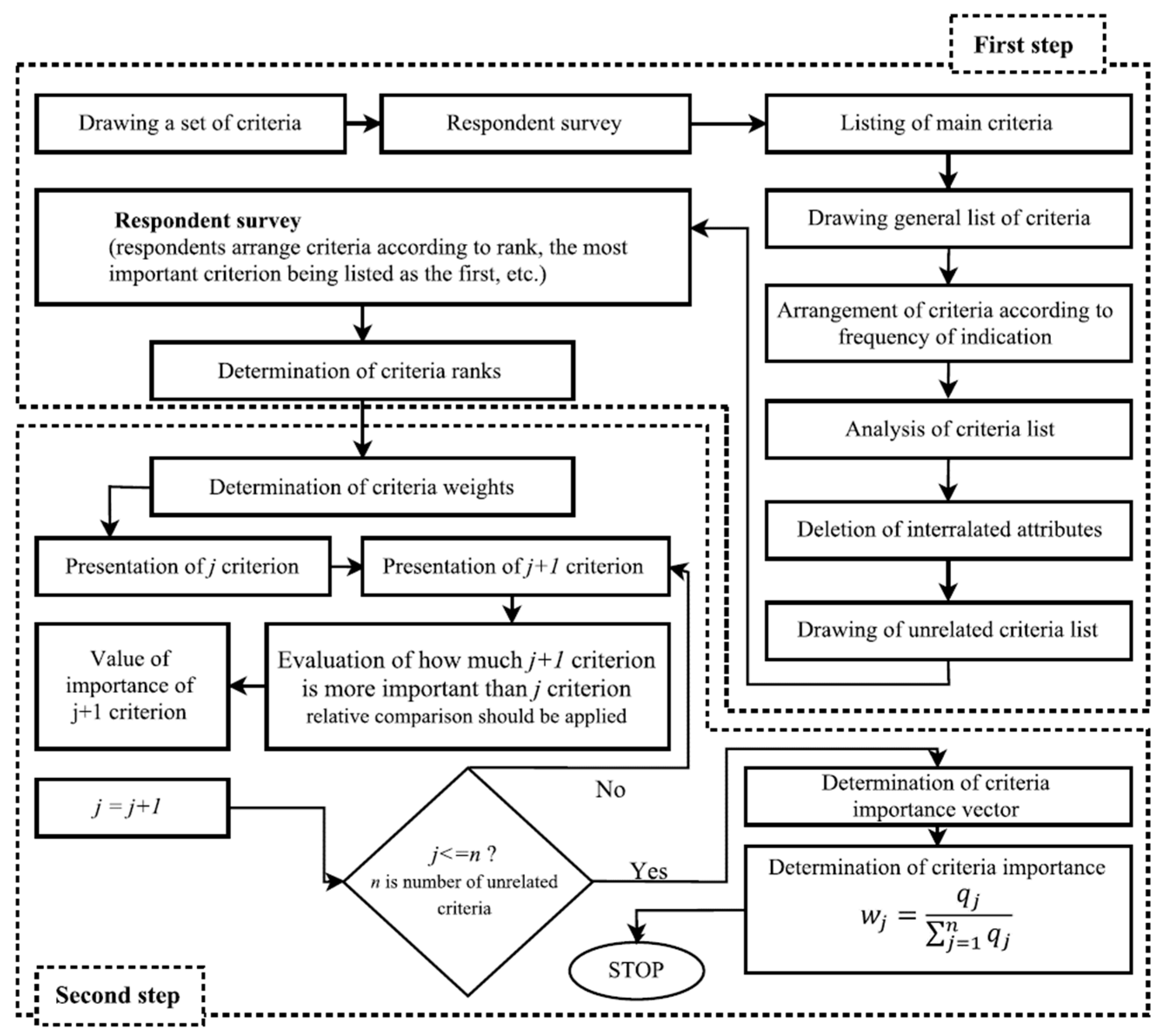
51], and others. In this research, the SWARA method was applied. The approach is uncomplicated, has clear and understandable logic, and is simple to use. The SWARA method consists of the two main steps. At the first round, a group of experts acts together. The team, based on the own knowledge, ordered criteria from the most significant (given rank 1), to the least significant, the last position. At the second step, each expert acts separately. Then, a systematic comparison between each more significant criterion is made with the less significant one. Each expert makes the contrasts in the second step based on his judgement.
Figure 1 shows the weight calculation procedure for the SWARA method. As the criteria weights in this MCDM problem represent the significance of each criterion, the authors asked five authorities of the constructor company to form the expert team for the SWARA method.
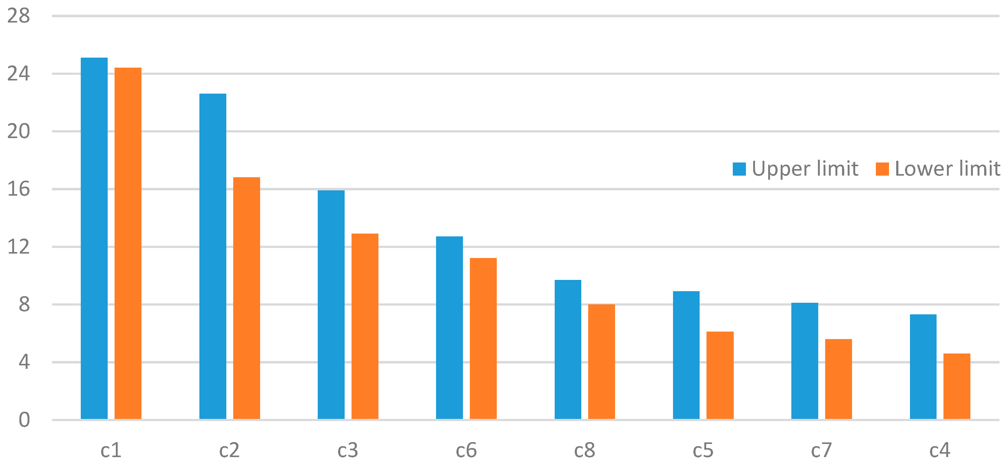
Table 2 shows the criteria weights obtained from the SWARA method in grey numbers. Lower and upper limits of each grey number are the lowest and highest amount received from the SWARA method among for each criterion, respectively.
Among the eight criteria defined for this problem cost, duration and uncertainty about final consequences are the most effective ones.
Table 2 shows that their cumulative weight is more than the five other criteria. In cases like ours, it is recommended to apply expert judgement to determine the values. The same as most cases in civil engineering, these values would not be precise enough with crisp numbers. Therefore, we calculated them in the shape of intervals. According to
Table 2 and
Figure 2, the range for some of the criteria weights like c
1, c
6, and c
8 are more close to a crisp number. It means that experts’ judgements about the effect of these criteria are similar. Moreover, Equation (8) can be derived. The priority order for the five most essential criteria may also be valid for crisp values.
3.3. Criteria Values Calculation
The next step to solve the proposed MCDM problem is to devise the grey decision-making matrix (GDMM). GDMM in discrete optimization problem consists of the preferences (values) of attributes (columns) for possible alternatives (rows):
The next step to solve the proposed MCDM problem is to devise the grey decision-making matrix (GDMM). GDMM in discrete optimization problem consists of the preferences (values) of attributes (columns) for possible alternatives (rows):
where
m—the number of alternatives,
n—the number of attributes describing each choice,
—a grey value representing the performance value of the
i alternative regarding the
j attribute.
The authors asked the constructor to calculate the criteria values because constructor authorities are the most familiar persons with the project.
Table 3 shows their completed GDMM and the requirements weight as the first row of the table.
Table 3 is the main entry for different methods in the following sections. The expert team which consisted of the project manager, site manager, and constructor authorities prepared the table. The direct cost of each solution calculated without uncertainty and the uncertainty related to C
1 is a part of the C
3 values. However, the expert team believed that crisp values for other criteria would not demonstrate a project’s real situation. Therefore, each member of the expert team completed the table based on his judgment and the maximum and minimum value of the team members for each criterion value is as the upper and the lower limit of a grey number. Each member of the expert team was asked to score the criteria C
3, C
4, C
5, C
6, C
7, and C
8, based on his judgement with a value among 1 (very low), 2 (small), 3 (medium), 4 (high), and 5 (very high). The upper and lower limit of a grey number for some of the C
2 values in
Table 3 is close to each other. That means that these grey numbers are almost crisp.
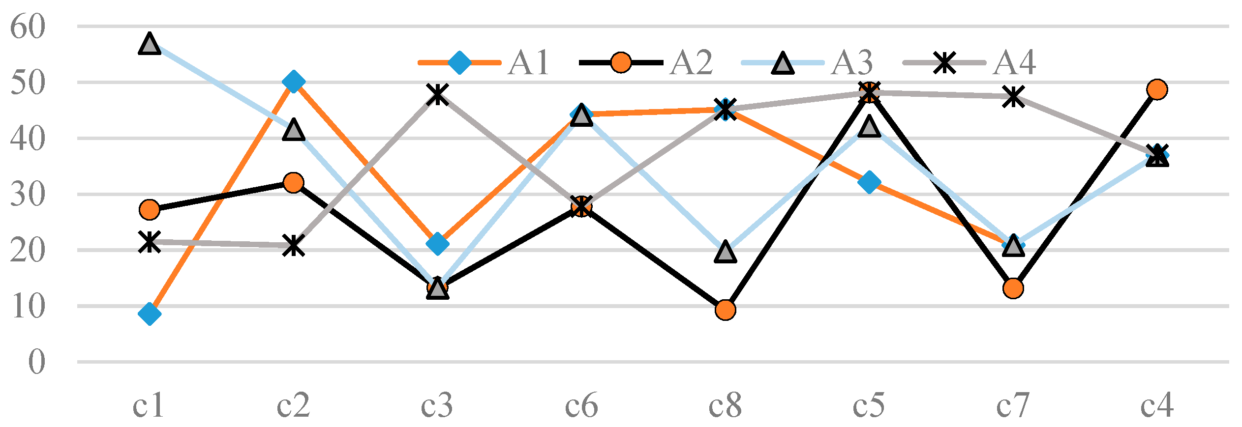
Figure 3 shows that no one of the alternatives is optimal according to all performance criteria.
4. Proposed Methods for MCDM Problem Resolution
The multiple attribute utility theory (MAUT) assigns a utility value to each action. This utility is a number representing the performance of the considered response. The functions of the multiple attribute utility theory are divided into three main types: Additive (ARAS—Additive Ratio Assessment, SAW—Simple Additive Weighting, SMART—Simple Multi Attribute Rating Technique, WSM—Weighted Sum Model, and others), multiplicative (WPM—Weighted Product Model, Geomean, MEW), and reference point (TOPSIS, VICOR) methods in different spaces. Multiplicative ones are more sensitive to criteria values than additive ones. Furthermore, reference point methods are very dependent on relative differences among criteria values, are suitable only for ranking and are not resistant to reversal ranking.
Thus, a decision-maker should check the ranking of alternatives according to these three utility function forms. In the present article, we apply the TOPSIS (reference point form), the ARAS (additive), and the Geomean (multiplicative). The grey numbers used as input parameters for these methods. Here, we explain the tools used in the present article.
4.1. The TOPSIS-G Method in Minkowski Space (TOPSIS-GM)
The TOPSIS method is the second most popular method among dozens of available MCDM methods. A large number of researchers argue that it is a mathematically very sound method. Despite this, it produces a ranking of alternatives, which is one of the rankest reversal unresisting (ranking of other options is changing, when Pareto non-optimal solutions are added, or removed).
Lin et al. [
52] proposed the following steps. Originally Hwang and Yoon [
53] introduced three versions of the TOPSIS method using Manhattan City block, Euclidean, and Minkowski space. Later, only a few publications were published using the TOPSIS method, not in Euclidean space. According to the authors’ opinion, it is better to use multidimensional space as different criteria to determine multi-criteria decision-making problems. The TOPSIS method with grey values is used to solve various issues [
54,
55,
56,
57,
58,
59,
60]. Meanwhile, the authors did not find any problems when Minkowski space is used.
A problem solution by TOPSIS-GM method could be described as a systemic procedure, as is shown below.
Step 1: Normalize the
matrix to obtain the normalized matrix
:
Normalized matrix is obtained through Vector normalization using Equation (11).
Step 2: Determine the positive and negative ideal alternative, and , respectively. is the optimal alternative based on optimal criteria values. is the possible alternative with the lowest value for each criterion among the values presented by considered alternatives.
Step 3: Calculate the values of normalized-weighted DMM:
where
is the weight for the
criterion, and
is the normalized value of the
th criterion of the
th alternative.
Step 4: Calculate separation measure from the positive and negative ideal alternatives,
and
, respectively:
where
and
are the normalized-weighted values of the
th criterion for the positive and negative ideal alternatives (
and
), respectively.
Step 5: Calculate the relative closeness
, as follows:
Then, the preference order of the alternatives presented as descending order of the value.
4.2. Additive Ratio ASsessment with Grey Numbers (ARAS-G) Method
Turskis and Zavadskas [
41] introduced the ARAS-G technique.
Step 1: The optimal alternative determination. The is the possible alternative determined by optimum criteria estimates (contrary to the TOPSIS or the COPRAS methods, where optimum values exist for selected to evaluation choices, or the best option is that which has the most significant multi-attribute utility function value).
Step 2: The normalized criteria values of matrix
calculated using the same Equation (8) as in the TOPSIS method (in ARAS method the main idea is that after criteria values are normalized, the ratio among normalized criteria values are the same as they were before normalization):
The cost type criteria normalized through Equations (17) and (18). It is a two-stage procedure, including the calculation of the changed decision-making matrix:
Step 3: Normalized-weighted DMM calculated by Equation (12).
Step 4: Transforming grey values into crisp values to obtain the utility degree of alternatives
:
Then, the options’ preference order presented as descending order of the : value.
4.3. The Geomean Method with Grey Numbers
The Geomean method is an MCDM utility function, and uses multiplication rather than addition to summarize criteria values. The Geomean method is an extension of the AHP multiplicative form. This approach is a useful tool when expecting the changes in relative preference order. A systemic procedure could be applied to develop it with grey number inputs:
Steps 1–3: Calculate the normalized-weighted DMM. The same normalized-weighted DMM of ARAS-G method used in this method.
Step 4: Determine the geometric mean of the alternatives
, as follows:
Then, the preference order of the alternatives ranked by descending order of the value.
5. Case Study Resolution
Table 4 and
Table 5A,B show the normalized DMM, using Equations (11), (17) and (18). Additionally, the positive and negative ideal alternatives corresponding to the TOPSIS-GM method are presented in the last two rows of
Table 4, and the optimal alternative corresponding to the ARAS-G method are shown in the last row of
Table 5A.
Then, normalized-weighted DMM (
Table 6 and
Table 7) were obtained by Equation (12) for both methods.
Using Equations (13)–(15) for TOPSIS-GM, Equation (19) for ARAS-G, and Equation (20) for the Geomean method, alternatives were prioritized. The last row of the
Table 8,
Table 9 and
Table 10 show the preferences of alternatives in the TOPSIS-GM, ARAS-G, and Geomean methods, respectively. Presenting the results of three methods, decision-makers (the contractor’s authorities) must choose the excellent alternative as the solution for the case study. Previously,
Figure 3 showed that none of the options are optimal according to all criteria values.
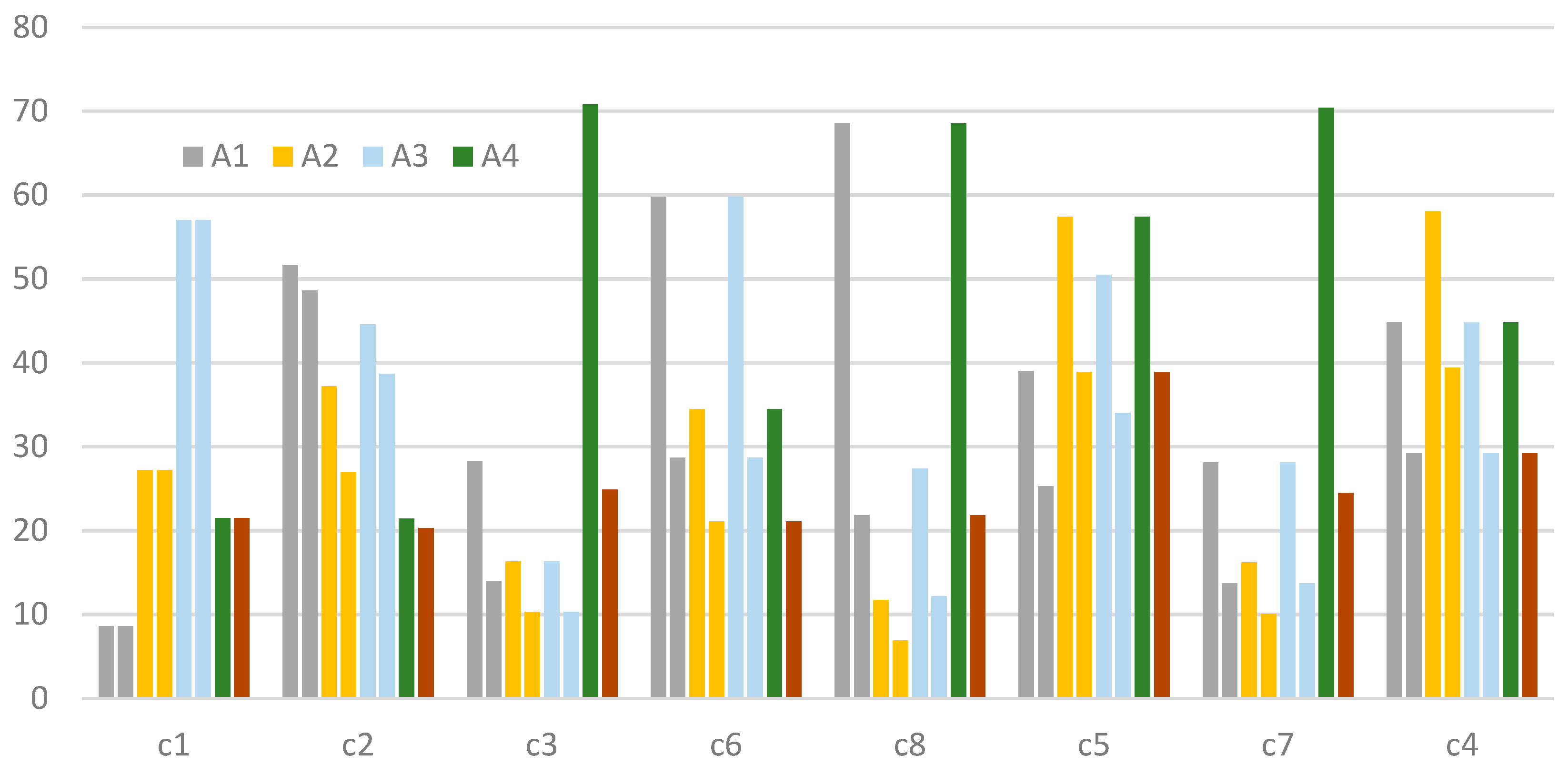
Focusing on
Figure 4, different uncertainty levels are present in the expert judgement. Upper and lower criteria values for the three most important criteria are equal (for C
1), or close to each other. However, other criteria values should be calculated using values at intervals. If the criteria are divided into four quarters, the two most important criteria are the cost (C
1) and duration (C
2) with a total weight of 45%. Possible future disputes (C
7) and related experiences in the past (C
4) with a total weight of 17% are the least important among the eight criteria under consideration. The remaining four criteria are moderate and have a total weight of 43%.
Here, grey numbers are used for their ease of use possibility. Structural change (A3) is the best-suggested alternative by TOPSIS-GM and ARAS-G methods. Besides, the Geomean method ranked it the second with a slight difference comparing with A4. Therefore, A3 is the optimal solution to the proposed case study. A3 has the lowest cost, and it is relatively fast to implement. These are the main two criteria.
The contractor implemented the result of the calculations practically. They applied the A3 as structural changes. After the application of these changes, the structure of the tower was completed within a short term. Structure completion had a significant effect on the target buyers and amplified the hopes for the soonest possible exploit from clients’ eyes. The project could even attract a remarkable number of the other tower’s potential buyers. This financial boost accelerated the activities’ progression more and more. At last, both contractors sold-out all of the units and immediately started the construction of their next tower in that area.
This model could be applied to a similar case when criteria are set, and weights and values updated in compliance with governing conditions.
6. Conclusions
Developing countries must promote the development of infrastructure, which has a positive effect on sustainable economic growth, to achieve a significant increase, except meeting basic needs. Sustainable construction addresses the ecological, social and economic issues of a building in the context of its community. Owner commitment, project delivery system, project team procurement, contract conditions, design integration, project team characteristics, and the construction process affect the schedule, cost, quality, and sustainable performance of green buildings and by managing these non-technical aspects, green buildings can be delivered successfully. Decision-makers must apply the appropriate change response whenever it is needed to maximize a project’s success. While proposing the best change strategy, decision makers are usually confronted with a multi-dimensional MCDM problem. This problem has different aspects of ambiguity and, using the crisp numbers, push the decision-makers away from reality. Similar issues need the application of fuzzy or grey numbers. The article presents a novel, multi-criteria change management response systemic procedure when change application in projects is needed. All the input values are grey numbers in the proposed change management model. The critical criteria, which affect the problem, and their weights, are subjective. Therefore, they were defined with expert judgment method, which is a part of the SWARA method. There is no one MCDM method which is the best for all case studies. Therefore, alternatives are ranked using the TOPSIS-GM, ARAS-G and Geomean methods with grey inputs. In the case study, four possible options and eight criteria (cost, duration, and some linguistic criteria) were defined.
A3 alternative is considered to be the best for TOPSIS-GM and ARAS-G methods. According to the Geomean method, it ranks second, and the difference from the best alternative is only 8%. It is, therefore, the most appropriate choice. The Geomean method considers A4 as the best, while according to the ARAS-G method, it ranks second, and the difference from the best is 14%, and according to TOPSIS-GM it ranks third, and the difference is 9%. Therefore, it is the second most suitable alternative after A3. A2 rates as the worst by ARAS-G and TOPSIS GM. According to the GEOMEAN method, it is the third concerning a 53% difference from the best-ranked alternative. The alternative is the worst according to the TOPSIS-GM and ARAS-G methods with the variations of 30% and 31% from the worst option. It can, therefore, be considered the worst alternative. A1 is supposed to be the worst under the TOPSIS GM method. According to the ARAS-G method, it occupies the third position, with a difference of 20%. Meanwhile, according to the Geomean G method, the worst third option has a 17% difference from the best. Therefore, it can be considered one of the worst available options.
According to the alternatives sum of ranks, the order of priorities is as follows: . Cost and time are the most important criteria. According to the problem solution results, the company made structural change. They shifted the concrete structure to a prefabricated steel structure and modified the specifications of the concrete used in shear walls and slabs for faster execution. The suggested alternative was implemented practically with positive results.
The model could be adopted to solve different construction delay change response problems by adding criteria, changing criteria weights, and alternatives.


 ,
, 

