Article

Influence of Extreme Events in Electric Energy Consumption and Gross Domestic Product

by
Fabrício Vieira
*,
Maurício Aparecido Ribeiro
,
Antonio Carlos de Francisco
and
Giane Gonçalves Lenzi
*
Federal Technological University of Paraná, Ponta Grossa 84016-210, Paraná, Brazil
*
Authors to whom correspondence should be addressed.
Sustainability 2019, 11(3), 672; https://doi.org/10.3390/su11030672
Submission received: 7 December 2018 / Revised: 15 January 2019 / Accepted: 19 January 2019 / Published: 28 January 2019

Abstract

:
The objective of this paper was to identify how extreme events can indicate periods of economic instability in variables from the economic and environmental context (per capita Gross Domestic Product (GDP), per capita electric energy consumption, and per capita carbon dioxide (CO2) emission). The research is limited to the population of the country (Brazil) and five cities of Paraná (Curitiba, Londrina, Maringá, Ponta Grossa, and Cascavel). Therefore, the major research interest was focused on finding information related to extreme events and other techniques that are used for interpretation of complex systems currently. The development was based on data collection. The results indicated that extreme events have influence in periods of economic instability. They also evidenced that there is greater correlation in GDP data/electric energy consumption than in GDP data/CO2 emissions or electric energy consumption/CO2 emissions.

1. Introduction

The world has witnessed several nations facing economic and financial crises. The causes of these crises are the most varied and differ according to the particularities of each country [1]. Nations considered exponents in financial terms, named advanced economies, due to their degree of security and return of investments, saw their finances pointing downward given the financial crises, which demonstrates the importance of the analysis and studies focusing on countries affected by instabilities [2].
Economic crises can be understood as temporary imbalances that significantly impact a nation and can even affect the financial stability of neighboring countries, besides influencing trading partners, businesses, employment and unemployment, inflation and others [3].
Several precise events can directly affect the economic and environmental variables. Therefore, extreme events directly affect the electric energy consumption. The global demand and consumption of energy, even though being able to reflect the heating up of the economy, are issues that have been calling the attention of several researchers, because, in terms of energy supply, electricity is a strategic resource for the development of cities and regions as a whole [4].
The Extreme Value Theory is a statistical and probabilistic technique used, in the analysis and interpretation of the so-called ‘extreme events’, in a time series [5]. In this context, extreme events are considered the values, in the time series, which stand out and differ, considerably, in absolute terms, from the average. This analysis includes mathematical observation of specificities and properties of these values that diverge, the so-called extreme events, also regarding the possibility of cyclical repetitions of these events in the course of time.
The self-organized criticality (SOC) analysis is based on cellular automata to annalize the behavior of the complex structures of the system. The occurrence of SOC is related to stationary statistical behavior. The analyzed systems of Energy consumption and CO2 emissions are not in steady behavior due to their dynamic behavior [6,7,8]. The theory of extreme values is basically the tendency of rare or extreme events to occur based on the distance between the mean and the median of the system. It also analyzes the sampling of rare values and the behavior of their distributions [9,10,11].
Peak Over Threshold (POT) is a method that addresses the tail estimation problem, through the generalized Pareto distributions, so that we can analyze the extreme events [12,13].
In this context, this study aims to evaluate the periods of economic and financial instability (GDP—Gross Domestic Product), and the electric energy consumption in Brazil’s cities and in the country as a whole, evaluating changes in these indexes, relating them to relevant global and regional contemporary events. The technique used will be the analysis of Extreme Events (EE) in a time series that outstands considerably in absolute terms of average or other parameters used, being unprecedented in this type of application.

2. Materials and Methods

2.1. Data Presentation

The search will be conducted to verify the correlation between extreme events and the electric energy demand of the five cities (Curitiba, Londrina, Maringá, Ponta Grossa and Cascavel) of Paraná, Brazil, in terms of population, and Brazil, as shown in Figure 1A) Cities of Paraná, research object. Source: [14]. Figure 1B) Brazil’s map emphasizing the Brazilian system of electric energy transmission. Source: [15].
Data of total electric energy consumption of these locations comprise the period from 1980 to 2014. The electric energy consumption includes the following categories: residential, industrial, commercial, and rural energy consumption; public power; and total consumption. Data were obtained from the Energy Company of Paraná (COPEL—Companhia Paranaense de Energia) [16]. Figure 1B shows the Brazilian system of electrical energy transmission in 2015. Gross Domestic Product data from these places were obtained from the World Bank [17].

2.2. Methodology

The analysis to verify the candidates to the points of the time series to extreme events is conducted in three steps: i) adjustment of a polynomial of degree N, 5 in this case, to the time series data; ii) calculation of the points of difference between the adjusted by the polynomial and that obtained by the time series. Therefore, we have the equation in which
δ ( t ) = P o ( t ) P a ( t )
P o ( t ) is the observed point (time series) and P a ( t ) is the point obtained by adjusting the polynomial; iii) calculation of the probability distribution of the sequence of points obtained by the difference of P o ( t ) and P a ( t ) . Such a probability distribution, the calculation of the full width at half maximum, will be a parameter of identification of candidates to extreme events in the time series.
Data analysis occurred through application of data in the program Grace and gnuplot and elaboration of Figures. The next section shows and discusses the results obtained in the research through analysis of extreme events in the data pool.

3. Results and Discussion

In Brazil, data from 1970 to 2014 indicate values for per capita GDP, per capita carbon dioxide (CO2) emissions and per capita electric energy consumption in time series, as shown in Figure 2.
Data indicate a growth, over the years, to all variables studied, indicating an influence among them. In addition, there is a drop in CO2 and a decrease in GDP around 2011 to 2014. On the other hand, this is not observed for the electric energy consumption. There are studies that establish a correlation between energy and the development of groups or institutions in general [18].
Figure 3 shows data of electric energy consumption in kW/h divided by the population, from 1970 to 2015, for the cities of Curitiba, Londrina, Maringá, Cascavel, and Ponta Grossa.
We observe that the curves of the total electric energy consumption have a similar behavior to all cities studied from 1970 to 2015. This means that this consumption is affected by the events in a similar manner. Therefore, we can indicate that some factors affect an increase or decrease in consumption. These events can be regional or global.
Figure 4 shows data relating a period-range and the extreme events/GDP/electric energy consumption in function of time. We observe that the extreme events influence the period in which they occur, i.e., they are not a precise phenomenon.
In particular, GDP values show a greater oscillation in specific periods: after 1980, after 1990, between 2000 and 2005, and discreet oscillation before 2010 and after 2010.

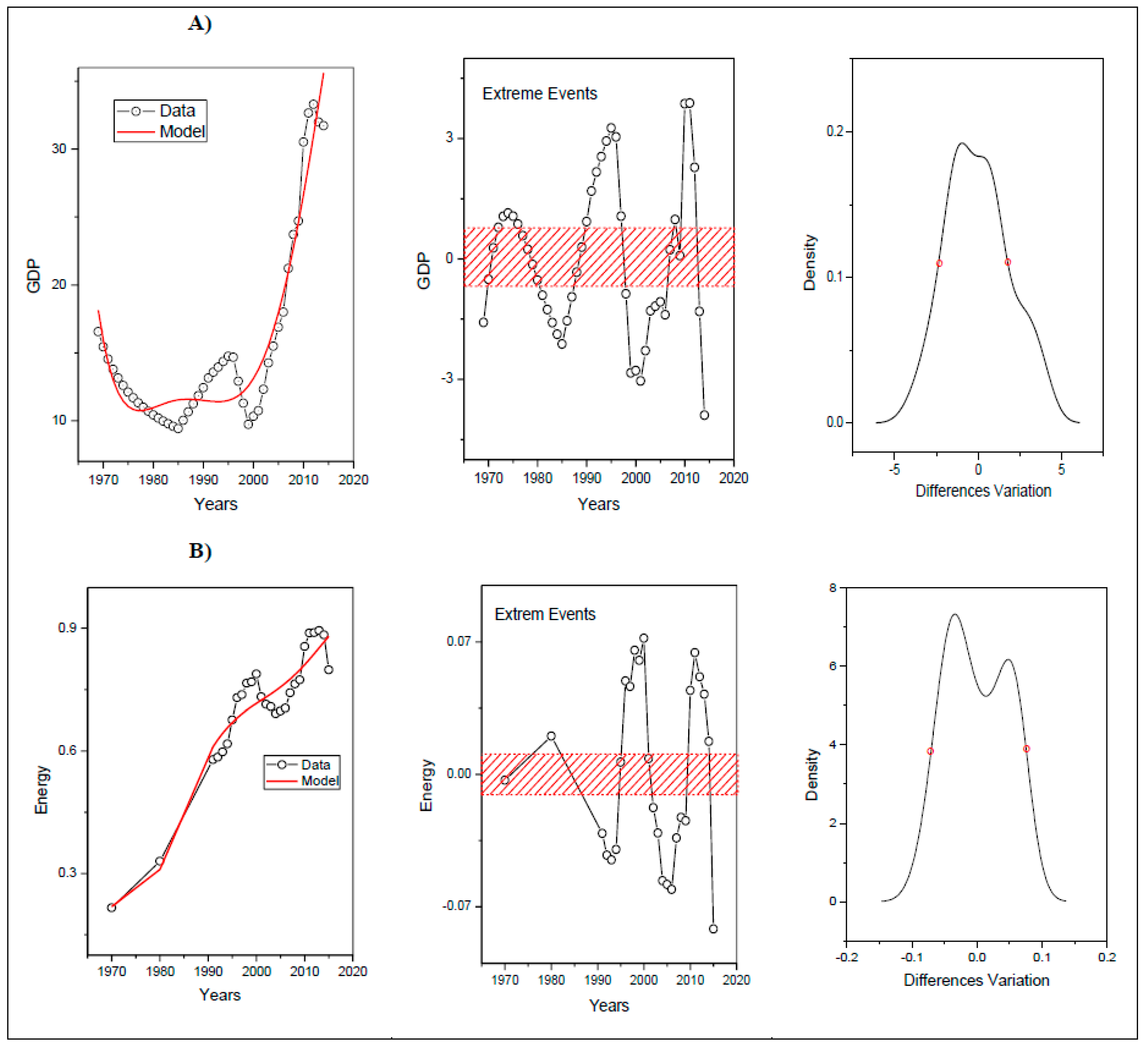
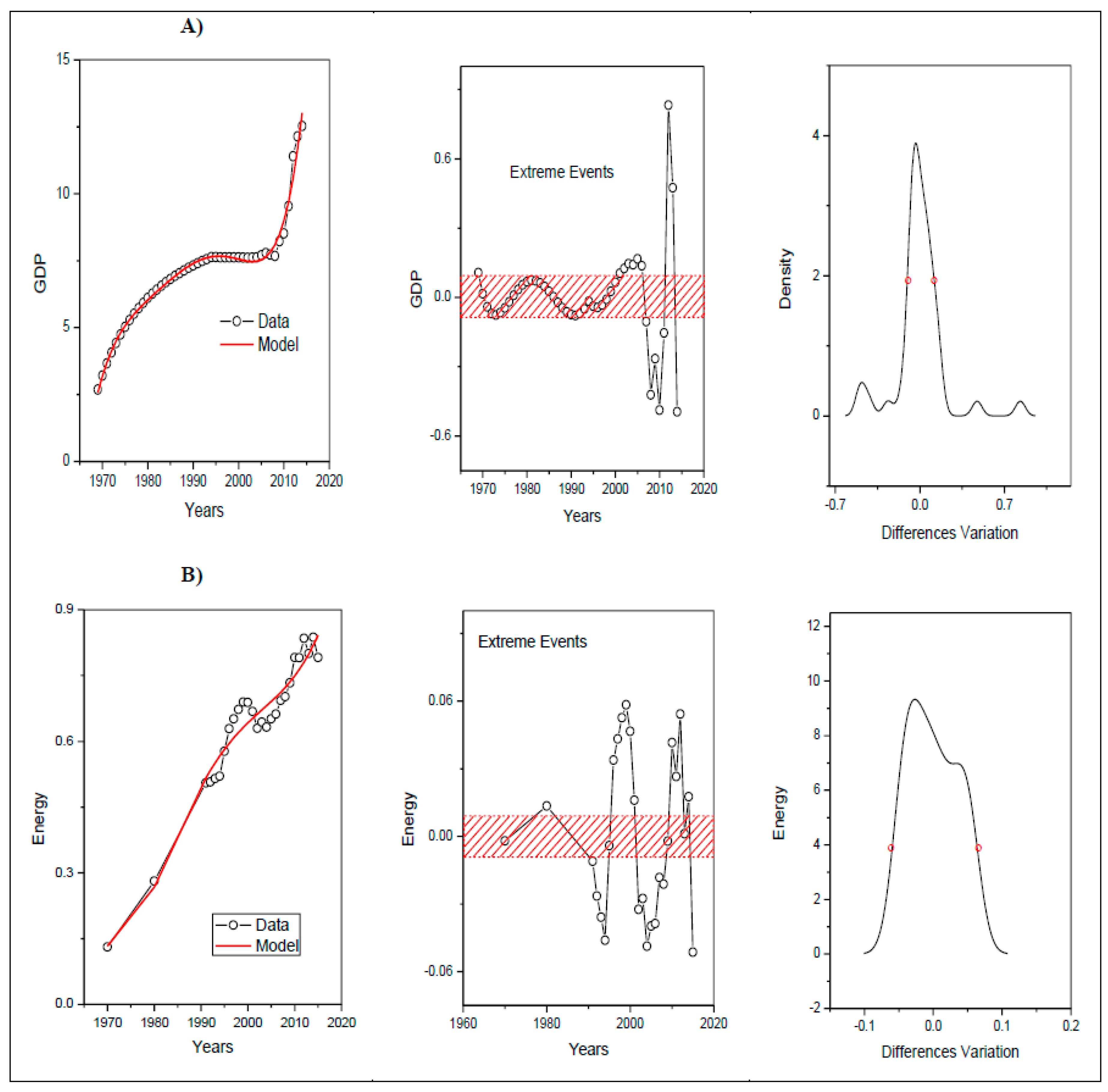
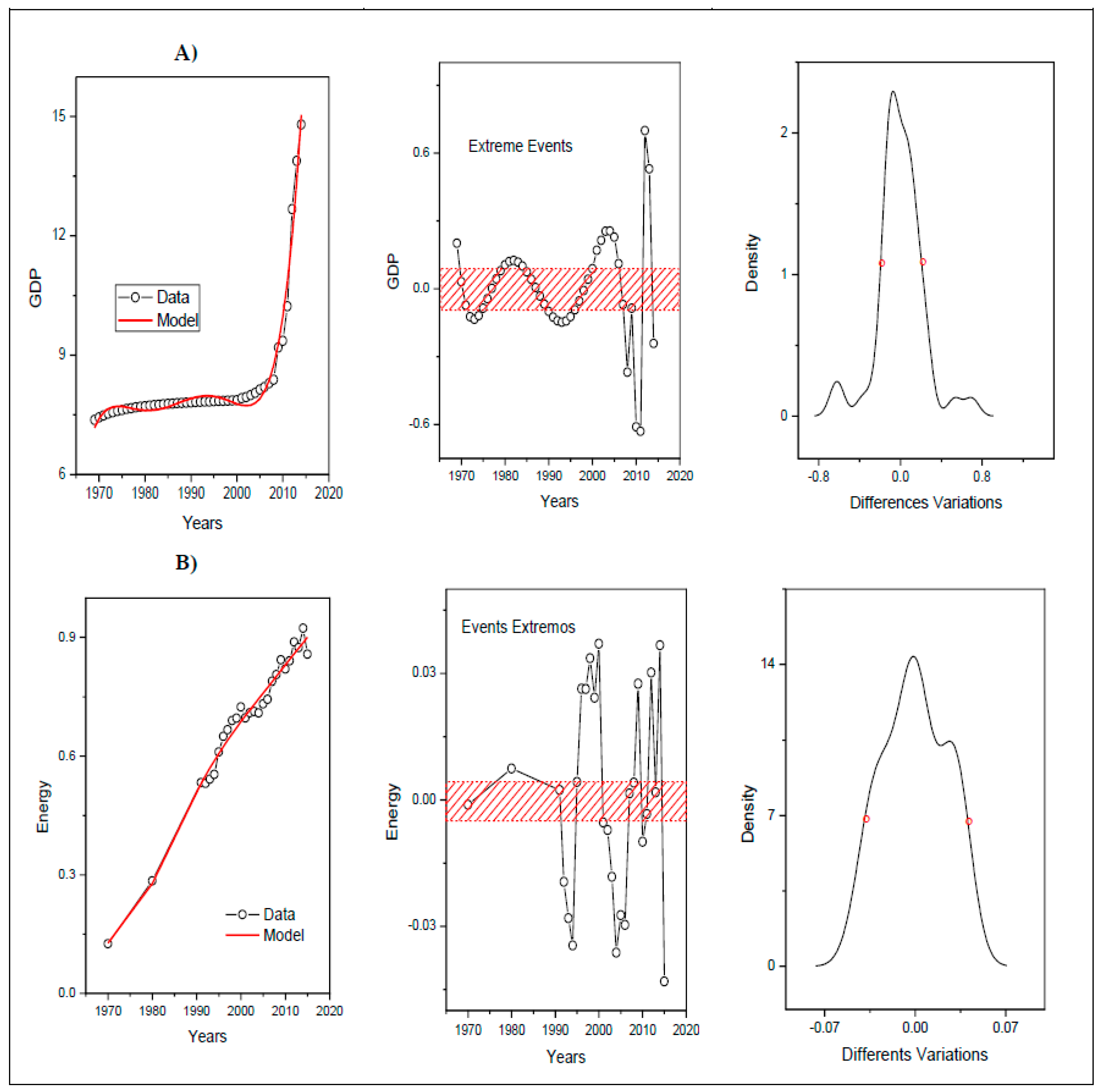
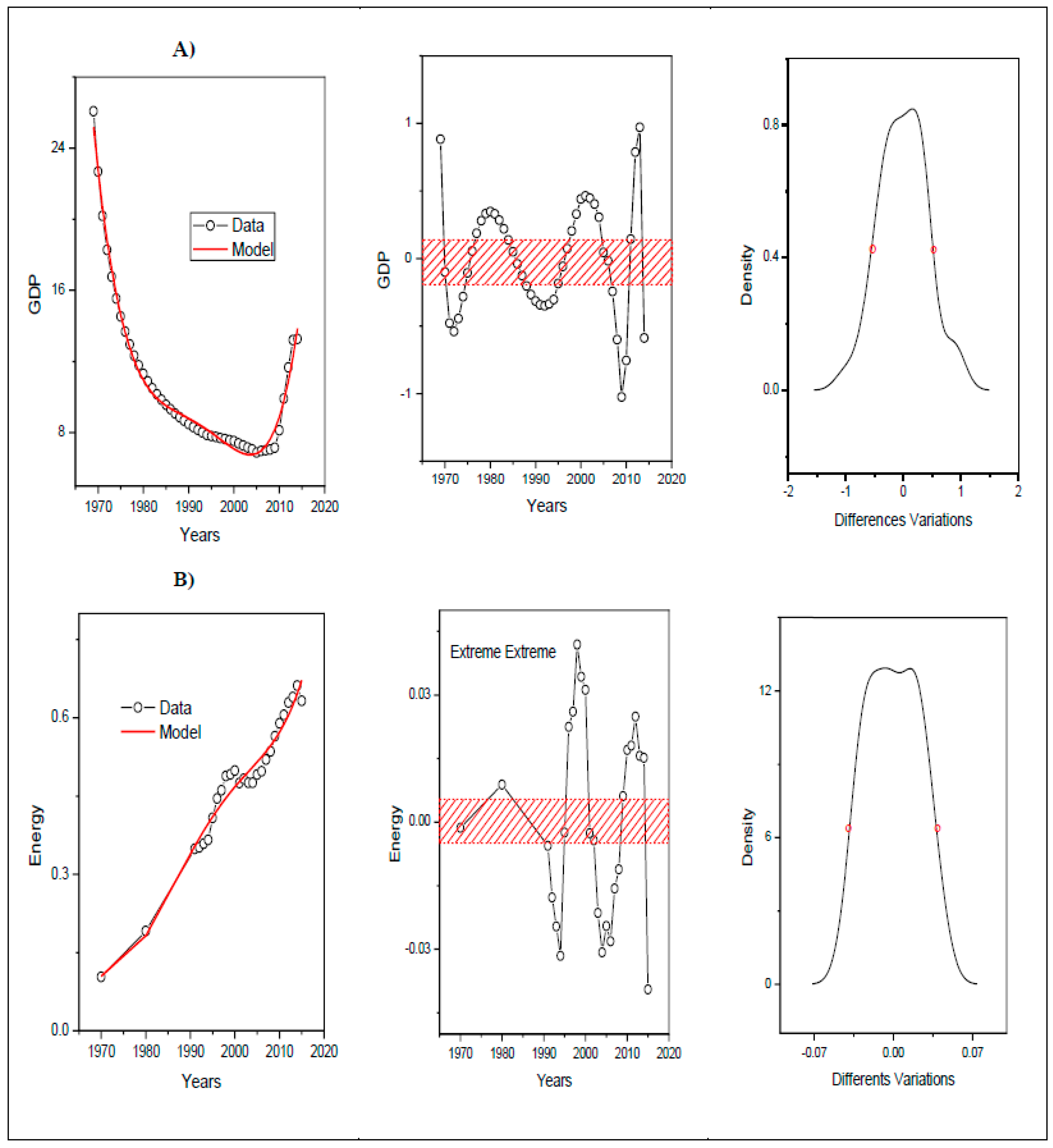
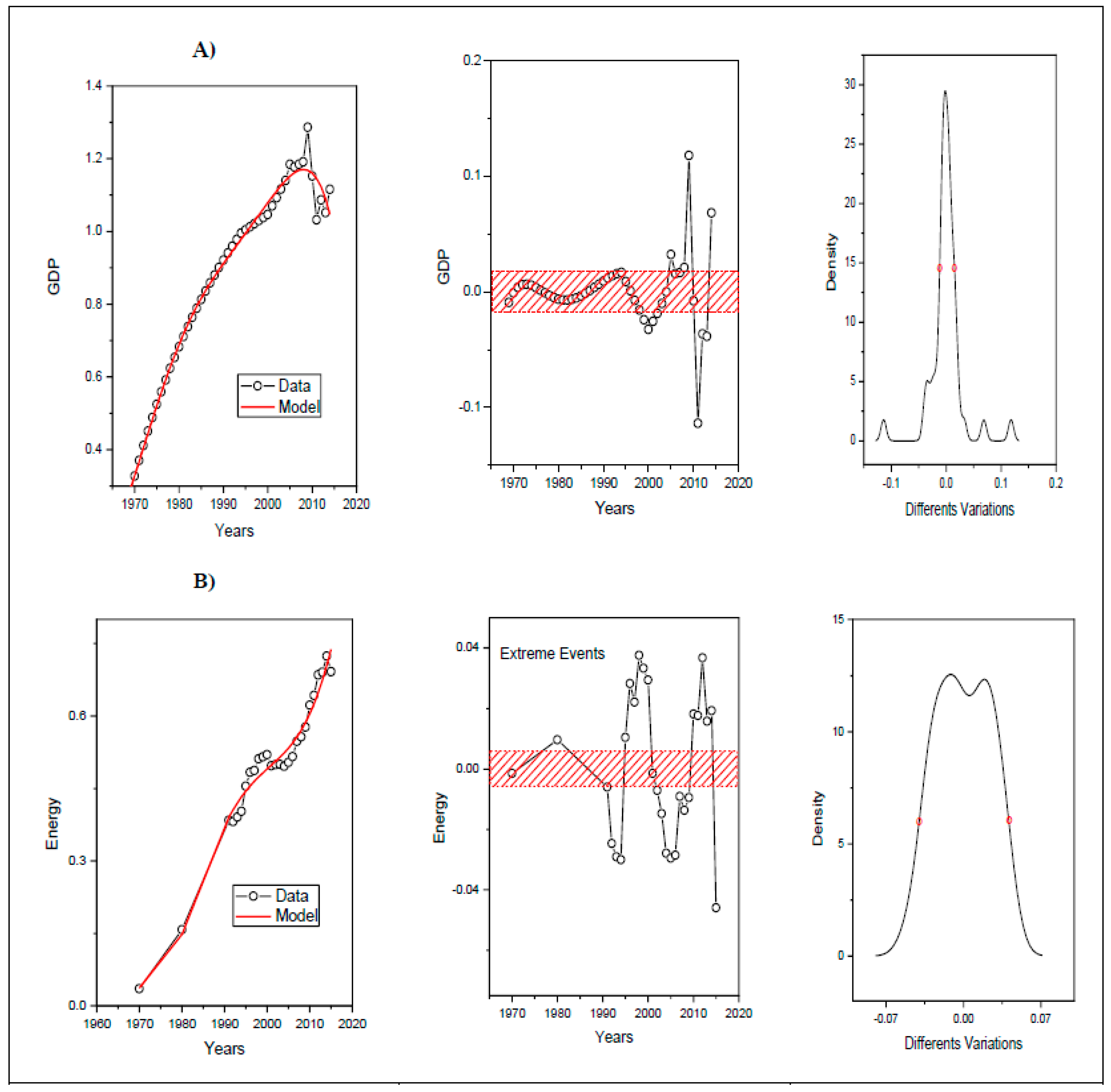
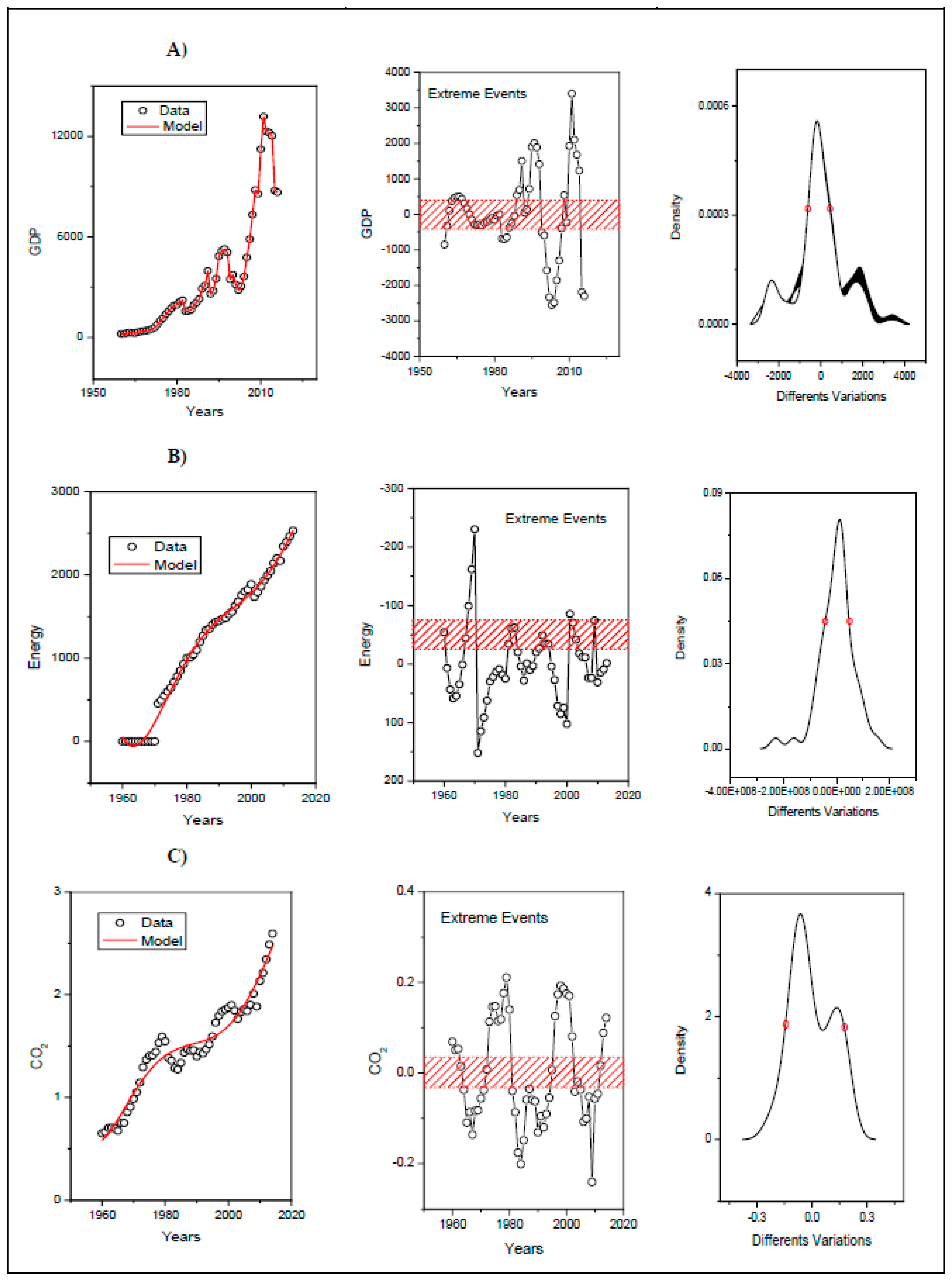
Analysis of Extreme Events

The data were acquired in the five largest cities in the state of Paraná, Brazil (Curitiba—Figure 5, Londrina—Figure 6, Maringá—Figure 7, Ponta Grossa—Figure 8, Cascavel—Figure 9), see Table 1. These data of total consumption of Electric Energy include the following uses: Residential, Industrial, Commercial, Rural, Public, Public Lighting, Public Service, Own (Energy Company). To observe in general, the study was conducted using data from Brazil. In this data the emission of CO2 was also included (Figure 10).

4. Discussion

4.1. Paraná

The 1970s were single period for Paraná, particularly due to the decline in the agricultural activities involving coffee production, a cultivation prevalent in the State in this period, and to the industrialization process, which began at this time. [19]. With the results obtained in Figure 5 to Figure 10, we can verify the occurrence of Extreme Events coinciding with the socioeconomic crises in the 1970s and 1980s, especially the crises that occurred in this period and which affected the price of oil barrels significantly, affecting the economy and the energy consumption, and these events occur and spread over a period.
Based on this industrialization, the State was expected to achieve economic, technological, and social development [20]. The main sources of income and development explored were agriculture, extractivism, and processing of yerba mate and wood, related to exportation and domestic consumption, mainly for the Brazilian Southeast [21].
The coffee production, developed in the North of the State, was in decline due to factors such as the modernization of agriculture, drops in market value and losses due to the weather, which resulted in unemployment and rural exodus [22]. In 1970, according to [23], p. 96 “the coffee still represented 27% of the cultivated area; in 1981, it fell to 8.5%; in the same period, the area cultivated with the six main grains (soybean, corn, bean, wheat, rice and peanut) increased from 61% to 85%.”
In the 1970s, the remarkable event is that in October 1973 the disputes involving petroleum exporting countries (PEC) began, which forbade the oil supply to the United States, Japan, and parts of Europe, that, at the time, imported from the Paraná State. This was, among others, the first crisis that occurred and went by the 1970s. This crisis also affected Paraná, since the activities of agriculture and importation/exportation suffer influence when the price of the oil oscillates.
We emphasize that the global events from this period, which significantly affected the GDP of Paraná, are the increase in the price of oil, the drop in exportations and the difficulties related to agriculture.

4.1.1. 1979 to 1987

In 1979, the significant economic and financial instability related to oil occurred. The Iran–Iraq war started in this period, in addition to the Iranian revolution previously started, convulsed the Arab world, and consequently affected the oil exports, a commodity that hit records in terms of price in this period. The 1979 crisis contributed to form the scenery of the 1980s in Brazil, marked by reduction of GDP, high interest rates, and inflation at high levels.
At the time when the first instabilities related to oil that surrounded the 1970s and 1980s began, Brazil, as well as other nations, had enormous dependence on this commodity. Since Brazil needed to import about 70% of the oil consumed in the country, in the most acute periods of the crisis, the value of this product had an increase of about 40%.
These factors naturally impacted the State of Paraná and its GDP, given that the State had as primordial economic activities, in general, agriculture, vegetal extractivism, and exportation [11], activities that are economically influenced by the price of a barrel of oil. With the increase in petroleum, there is consequently an increase in expense of related fuels and other expenditures related to the petroleum consumption. The oil crisis affected the State in such a way that rationing measures were adopter for fuels such as gasoline, which accompanied the rise of the oil prices.
Some highlighted global events from this period, which significantly affected the GDP of Paraná, are rises in the price of oil, which had already begun in the 1970s; the drop in exportations (the main countries that imported from Paraná were in financial difficulties); and excessive dependence in relation to oil.

4.1.2. 2000s

In the 2000s, Paraná was still remarkable considering exportations, extractivism, and agribusiness. Also, the agribusiness and extractivism increasingly had more promising prospects due to the rising foreign market and appreciation of these products in the market.
However, this State, as well as Brazil, was affected by instabilities in periods related to extreme events pointed in the figure, such as the Asian financial crisis (1997), the Russian crisis (1998), the Brazilian crisis (1999), and the American crisis (2000), in the year after the terrorist attacks on the USA (2001) and the crisis in Argentina (2001–2002) that were predominant factors affecting exportations and agribusiness in the State and causing oscillations in the GDP of Paraná.

4.1.3. 2009

In 2009, Paraná suffered the influences of global instabilities initiated with European countries and with the United States. With the most prominent activities in the State being agriculture and vegetal extractivism, the greatest economic crisis in the US since 1929, and intense periods of economic instability in the European Union, Paraná suffered the impacts of these crises, reflected also in its GDP.
Exportations were specially affected since nations importing goods from the State, as European countries were undergoing severe financial instability.

4.2. Brazil

4.2.1. 1979 to 1987

After 1980, Brazil, within the global context, suffered the effects resulting from conflicts in the East (in 1979). In addition, this region was an exponent of oil, which resulted in a global crisis. Nations, in general, felt the impact of this crisis; however, developing countries were the most affected, as they had to handle the high expenses due to oil prices, subsequent rises of inflation, and burden of external debt. Within the internal political context, Brazil began the redemocratization of the country, which hitherto was under the regime of the Military Dictatorship, since 1964.
In 1979, again, conflicts in the East (the Islamic Republic of Iran was created) and the fact that this region is exponent, in terms of oil supply, resulted in a global financial crisis. Nevertheless, the 1973 crisis was a warning to Western countries to question their dependence on oil. The drop in the offer of this commodity resulted, again, in the significant rise of the prices. Nations, in general, felt the impact of this crisis; however, developing countries were the most affected, as they had to handle the high expenses due to oil prices, subsequent rises of inflation, and burden of external debt.
The 1980s was marked by two financial crises of greater significance. In 1980, again, a conflict between Iraq and Iran caused a quite expressive high in the price of the oil barrel (US$ 40 a barrel, index never achieved in any of the 1970s crises). This new high in prices caused Western countries to search oil reserves for their own exploitation.
In 1987, a crisis broke out in the American stock exchanges and expanded to other regions, such as Europe and Asia, and affected significantly developing economies, such as Brazil, that were not able to pay the external debt.
The following figure represents the variation in GDP of some countries over the years. GDP annual growth rate at market prices based on local constant currency. “GDP is the sum of gross value added by all resident producers in the economy plus any product taxes and minus any subsidies not included in the value of the products. It is calculated without making deductions for depreciation of fabricated assets or for depletion and degradation of natural resources” [24]. We highlight the intense oscillations in periods of instability, same period in which this oil crisis broke out Figure 11.
After 1990, Brazil had rising values for variables of per capita CO2 emissions and per capita electric energy consumption, with little noise. As for per capita GDP values, we observed a remarkable drop in values after 1993, a probable influence of the financial crises taking place at the time, as the Mexican crisis broke out notably in 1994.

4.2.2. 2000s

The Mexican crisis was the first among the four crises that occurred in the 1990s. In 1994, Mexico adopted a system named crawling peg. However, there was a sharp devaluation of the peso, which, together with the rising Mexican inflation, culminated in the crisis that spread to other nations through debt instruments, a consequence named “Tequila effect”. The effects of this crisis were felt worldwide and in Brazil.
Brazil, in 1999, would be prominent when viewing its currency (real) suffer strong devaluation in the international market, episode known as the Brazilian financial crisis. The Real Plan, implemented in 1994, managed to stabilize what was, at that time, a lasting Brazilian difficulty and that significantly affected the country’s economy: the inflation.
In 1997, according to [25], the one that became known as “the crisis of the Asian giants” was started with successive devaluations of the currencies of nations forming this block, starting by Thailand and extending to Korea, Malaysia, and others. The effects of this crisis spread and affected several countries (Australia, Mexico, England, Japan, Brazil), in addition to causing bankruptcy of banks and indebtedness of companies. [26] Added to that, among the possible causes of this crisis, there are highlighted: the plan, used by the ‘Asian Tigers’, to be linked to the American currency; external indebtedness; and exchange of favors between the government and the private initiative. This crisis was contained only after interventions by the International Monetary Fund (IMF). Figure 12 shows the variation in the GDP value in some selected nations in this period.
According to [27], in 1998, Russia, that had already suffered the impacts of previous crises and having as main causes the monetary issues and currency devaluation, underwent a period of economic turmoil. The Russian stock exchange showed deficits as well as others around the world. Only in 1999 was there a stabilization of this situation and signs of improvement of the Russian economy and the nation in general.
The stock exchange, National Association of Securities Dealers Automated Quotations (NASDAQ), which has great representativeness among computing, technology and telecommunications companies suffered a sharp drop in 2000, being the first of six financial crises that the world experienced in the 21st century. In only three years, this crisis of companies in the field of technology led to financial losses and bankruptcy of thousands of small companies, in addition to some giant companies in the area of computing and telecommunications. The attack on the Twin Towers of the World Trade Center in New York would occur in the next year, with 3,000 deaths. This fact culminated in the 2001 crisis with expressive drops in stock exchanges of several nations.
Within the same period, from 2001 to 2002, Argentina suffered the adjustment measures adopted by the president. These measures would generate high unemployment rates and an international climate of mistrust. In the end of 2001, Argentina suspended the payment of the foreign debt of 100 billion dollars.
Figure 13 shows the unemployment percentage in Brazil and in other countries in this period of imbalance. Unemployment, according to the [28], refers to the supply of labor of unemployed people, but available for and seeking work. We highlight in Figure 13 the expressive variation of this index in cycles of financial instability.

4.2.3. 2009

In 2008, the US were at the center of the major economic crisis since the 1929 crisis. The highlights in this crisis were the so-called ‘housing bubble burst’ (lessening in evaluation for concession of mortgages, generating highs in nonpayments) and the massive declaration of insolvency by financial institutions. Among the causes of this crisis, there is the negligence in risk assessments in financial investments.
This crisis went by some American governments (George W. Bush and Barack Obama), who invested by injecting massive amounts of money into economic recovery programs.
The European Union, a social, political, and economic cluster, which accounts for a significant portion of the global GDP, suffered a monetary crisis in 2009. It was initially motivated by Greece’s sharp and successive deficits, which generated distrust on the capacity of several member countries, significantly and directly affecting countries as Portugal, Spain, Ireland, and Italy, which caused a significant drop in the appreciation of the euro against other currencies.
According to the World Bank data, at the peak of the crisis, countries, as Italy, had accumulated percentage deficits in relation to GDP of 11.5% in Spain and 8.5% in Portugal. The percentages of unemployment rates reached 18% in Greece, 15% in Ireland and 21% in Spain.
Finally, in 2015, the Brazilian economic crisis would be characterized by certain factors which showed marks of economic instability. The Table 2 below summarizes the EE in the sample by location, year, and variable studied.
It is still relevant to present the EE in the sample in a different way so that a better understanding of the results can be obtained. It is imperative to point out that the most significant EE observed are contemporaneous with periods of financial economic mismatch, as show in Table 3.

5. Conclusions

Under a global perspective, culture, economy, imports/exports oscillated and were influenced by these periods of instability. These oscillations justify the extreme events in the sample and, therefore, correspond with the global context at the time. They also evidenced that there is greater correlation in GDP data/electric energy consumption than in GDP data/CO2 emissions or electric energy consumption/CO2 emissions. The extreme events in the variables per capita GDP, per capita electric energy consumption, and per capita CO2 emissions, broke out in periods related to economic crises. It observed that developing countries have a more pronounced influence in the studied variables, and these are related.

Author Contributions

F.V., M.A.R., A.C.d.F. and G.G.L. contributed to the design and implementation of the research, to the analysis of the results and to the writing of the manuscript.

Funding

This research received no external funding.

Conflicts of Interest

The authors declare that there is no conflict of interest regarding the publication of this paper.

References

  1. Epstein, G.A. Financialization and the World Economy; Edward Elgar Publishing: Cheltenham, UK, 2005. [Google Scholar]
  2. Hobsbawm, E.J. Age of Extremes: The Brief Century XX, 1914–1991, 2nd ed.; Letter Company: São Paulo, Brazil, 1995; 598p, ISBN 857164468-3. [Google Scholar]
  3. Brener, J. 1929: The Crisis that Changed the World, 1st ed.; Ática, 20th Century Retrospective Collection: São Paulo, Brazil, 1996. [Google Scholar]
  4. ANEEL—National Agency of Energy Electricity. ANEEL: Brasília, Brazil, 2002; 153p. Available online: http://www2.aneel.gov.br/arquivos/pdf/livro_atlas.pdf (accessed on 20 June 2017).
  5. Heffernan, J.E.; Stephenson, A.G. Ismev: An Introduction to Statistical Modeling of Extreme Values. 2018. Available online: https://cran.r-project.org/web/packages/ismev/ismev.pdf (accessed on 20 June 2017).
  6. Bak, P.; Tang, C.; Wiesenfeld, K. Self-organized criticality. Phys. Rev. A 1998, 38, 364. [Google Scholar] [CrossRef]
  7. Bak, P.; Tang, C.; Wiesenfeld, K. Self-organized criticality: An explanation of the 1/f noise. Phys. Rev. Lett. 1987, 59, 381. [Google Scholar] [CrossRef] [PubMed]
  8. Bak, P.; Chen, K. Self-organized criticality. Sci. Am. 1991, 264, 46–53. [Google Scholar] [CrossRef]
  9. Beirlant, J.; Goegebeur, Y.; Segers, J.; Teugels, J.L. Statistics of Extremes: Theory and Applications; John Wiley & Sons: Hoboken, NJ, USA, 2006. [Google Scholar]
  10. Oliveira, J.T. Statistical Extremes and Applications; Springer: Berlin, Germany, 2013; Volume 131. [Google Scholar]
  11. Katz, R.W. Statistics of extremes in climate change. Clim. Chang. 2010, 100, 71–76. [Google Scholar] [CrossRef]
  12. Smith, R.L. Threshold methods for sample extremes. In Statistical Extremes and Applications; Springer: Dordrecht, The Netherlands, 1984; pp. 621–638. [Google Scholar]
  13. Méndez, F.J.; Menéndez, M.; Luceño, A.; Losada, I.J. Estimation of the long-term variability of extreme significant wave height using a time-dependent peak over threshold (pot) model. J. Geophys. Res. Oceans 2006, 111. [Google Scholar] [CrossRef]
  14. IBGE. Country Information. Available online: https://paises.ibge.gov.br/#/pt/pais/brasil/info/sintese (accessed on 27 October 2017).
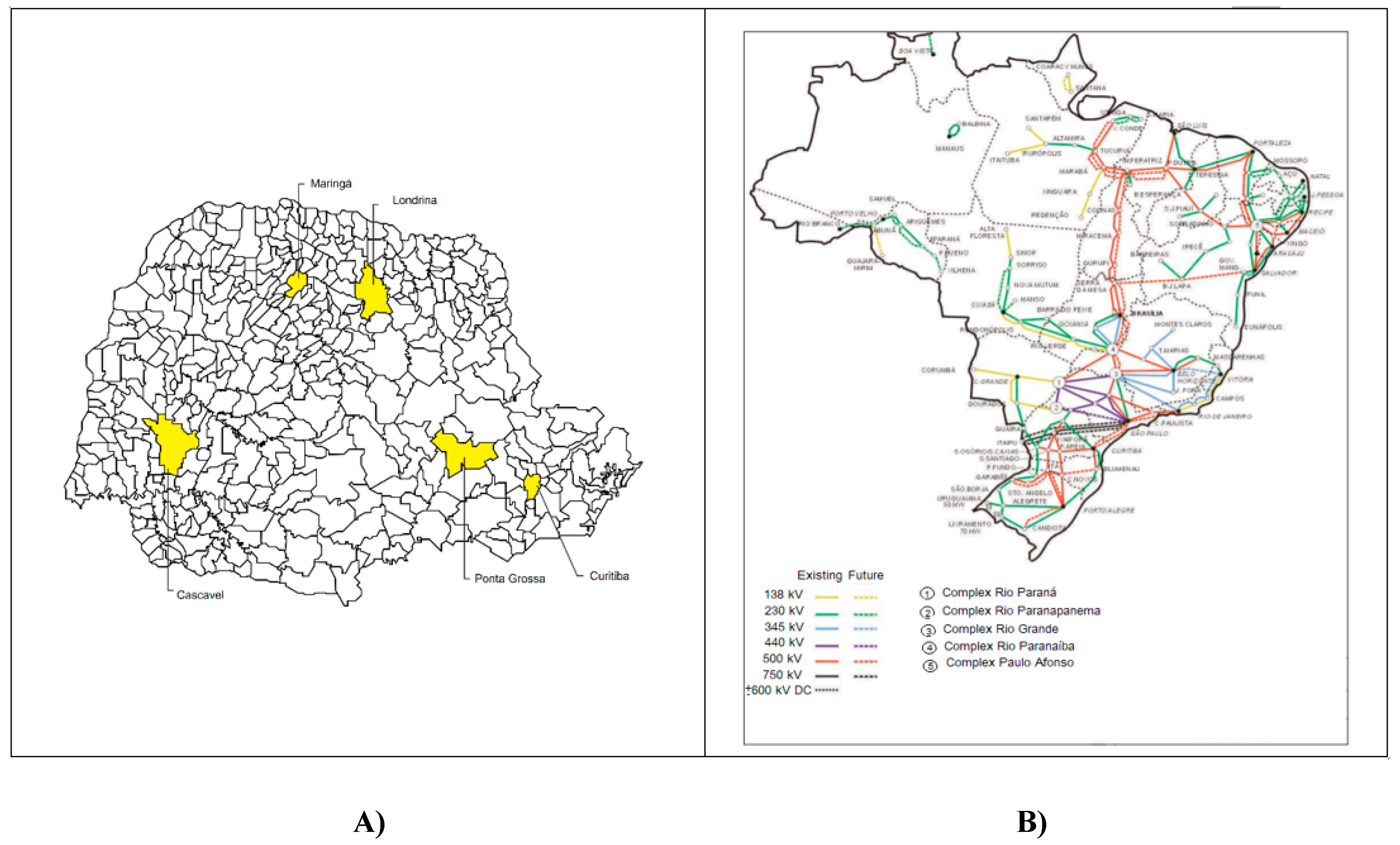
  15. ANEEL. Map of the National Electric Power Transmission System. Available online: http://www.aneel.gov.br/transmissao5 (accessed on 20 June 2017).
  16. COPEL—Company Paranaense of Energy. Available online: www.copel.com (accessed on 20 June 2017).
  17. Word Bank. Country Database. Available online: http://databank.worldbank.org/data/reports.aspx?source=2&series=SP.POP.TOTL&country=# (accessed on 25 June 2017).
  18. Fix, B. Energy and institution size. PLoS ONE 2017, 12. [Google Scholar] [CrossRef] [PubMed]
  19. Trintin, J.G. The New Economy of Paranaense: 1970 to 2000; Eduem: Maringá, Brazil, 2006. [Google Scholar]
  20. Oliveira, D. Urbanization and Industrialization in Paraná; SEED: Curitiba, Brazil, 2001. [Google Scholar]
  21. Leão, I.Z.C.C. Paraná in the Seventies; IPARDES/CONCITEC: Curitiba, Brazil, 1989.
  22. Volaco, G.; Baggio, E.C.; Shibata, E.K.; Lourenço, G.M. Paraná Economy: Recent Performance and Short-Term Scenarios; Conjunctural Analysis; IPARDES: Curitiba, Brazil, 1991.
  23. Magalhães Filho, F.B.B. The New Economic Profile of Paraná. FEE Econ. Indic. 1993, 21. Available online: https://revistas.fee.tche.br/index.php/indicadores/article/view/588/827 (accessed on 20 September 2017).
  24. Word Bank. GDP per Capita (Current US$). Available online: https://datamarket.com/data/list/?q=gdp+spain+provider%3Aworld-bank (accessed on 25 June 2017).
  25. Walter, A.W. Governing Finance; Cornell University Press: New York, NY, USA, 2008. [Google Scholar]
  26. Fidrmuc, J.; Korhonen, I. The impact of the global financial crisis on business cycles in Asian emerging economies. J. Asian Econ. 2010, 21, 293–303. [Google Scholar] [CrossRef] [Green Version]
  27. Tong, H.; Wei, S.-J. The composition matters: Capital inflows and liquidity crunch during a global economic crisis. Rev. Financ. Stud. 2011, 24, 2023–2052. [Google Scholar] [CrossRef]
  28. Word Bank. Unemployment, Total (Modeled ILO Estimate). Available online: https://data.worldbank.org/indicator/SL.UEM.TOTL.ZS (accessed on 25 June 2017).
Figure 1. (A) Cities of Paraná, research object. Source: IBGE - Brazilian Institute of Geography and Statistics (2017). (B) Brazil’s map emphasizing the Brazilian system of electric energy transmission. Source: ANEEL—National Agency of Energy Electricity (2017).
Sustainability 11 00672 g001
Figure 2. Gross Domestic Profit (GDP), CO2 emissions, and electric energy consumption in Brazil in per capita values in a time series (1970 to 2014). Source: own authorship (2018).
Sustainability 11 00672 g002
Figure 3. Total electric energy consumption (per capita) per time. Source: own authorship (2018).
Sustainability 11 00672 g003
Figure 4. Extreme events (electric energy consumption/GDP). Source: own authorship (2018).
Sustainability 11 00672 g004
Figure 5. Acquisition of extreme events for Curitiba. (A) GDP; (B) Energy. (1) Adjustment of polynomial; (2) points of difference between that adjusted by the polynomial and that obtained by time series; (3) probability distribution of sequence of points obtained by the difference from P o ( t ) and P a ( t ) . Source: own authorship (2018).
Sustainability 11 00672 g005
Figure 6. Acquisition of extreme events for Londrina. (A) GDP; (B) Energy. (1) Adjustment of polynomial; (2) points of difference between that adjusted by the polynomial and that obtained by time series; (3) probability distribution of sequence of points obtained by the difference from P o ( t ) and P a ( t ) . Source: own authorship (2018).
Sustainability 11 00672 g006
Figure 7. Acquisition of extreme events for Maringá. (A) GDP; (B) Energy. (1) Adjustment of polynomial; (2) points of difference between that adjusted by the polynomial and that obtained by time series; (3) probability distribution of sequence of points obtained by the difference from P o ( t ) and P a ( t ) . Source: own authorship (2018).
Sustainability 11 00672 g007
Figure 8. Acquisition of extreme events for Ponta Grossa. (A) GDP; (B) Energy. (1) Adjustment of polynomial; (2) points of difference between that adjusted by the polynomial and that obtained by time series; (3) probability distribution of sequence of points obtained by the difference from P o ( t ) and P a ( t ) . Source: own authorship (2018).
Sustainability 11 00672 g008
Figure 9. Acquisition of extreme events for Cascavel. (A) GDP; (B) Energy. (1) Adjustment of polynomial; (2) points of difference between that adjusted by the polynomial and that obtained by time series; (3) probability distribution of sequence of points obtained by the difference from P o ( t ) and P a ( t ) . Source: own authorship (2018).
Sustainability 11 00672 g009
Figure 10. Acquisition of extreme events for Brazil. (A) GDP; (B) Energy. C) CO2. (1) Adjustment of polynomial; (2) points of difference between that adjusted by the polynomial and that obtained by time series; (3) probability distribution of sequence of points obtained by the difference from P o ( t ) and P a ( t ) . Source: own authorship (2018).
Sustainability 11 00672 g010
Figure 11. Variation of GDP (annual %) in selected countries. Source: own authorship (2017).
Sustainability 11 00672 g011
Figure 12. GDP variation (in US$) in some countries. Source: own authorship (2017).
Sustainability 11 00672 g012
Figure 13. Total unemployment in % related to the total workforce in some countries. Source: own authorship (2017).
Sustainability 11 00672 g013
Table 1. Extreme Events indicated by city and variable studied.
LocalityExtreme Events (EE) x VariableYears that Presented EE above the Width at Half Height:Years that Presented EE below the Width at Half Height:
CuritibaEE(Extreme Events) GDP1991–19961970, 1982–1986, 199–2006, 2013–2014
EE electricity consumption1995–2000, 2010–20131991–1995, 2004–2008
LondrinaEE GDP1970, 1980–1985 (discreet), 2002–2007 (strong), 2012–2013 (strong)1972–1975 (leve), 1990–1995 (leve), 2008–2011 (strong), 2014 (strong)
EE electricity consumption1995–1999, 2009–20111991–1993, 2002–2008, 2014
MaringáEE GDP1970, 1979–1985 (discreet), 2000–2007 (strong), 2013–2014(strong)1973–1976, 1990–1997, 2010–2011, 2015
EE electricity consumption1997–2000, 2007, 20091992–1995, 2004–2007, 2015
Ponta GrossaEE GDP1970, 1980–1984, 2000–2005, 2013–20141971–1975, 1989–1996 (discreet), 2008–2010 (strong), 2015
EE electricity consumption1995–2000, 2011–20141992–1994, 2004–2009, 2015
CascavelEE GDP2005–2010, 20151998–2002 (discreet),
EE electricity consumption1996–2000, 20121991–1993, 2004–2006, 2015
BrazilEE GDP1986, 1989–1992, 2010–2014,1961–1963, 1973–1986, 1991–1992, 2005–2010, 2015–2016
EE electricity consumption1960, 1967–1970, 1980–1982, 2000–2002, 20101962–1965, 1971–1976, 1996–2000, 2007–2010
EE Emissions of CO21973–1980, 1997–2003, 2011–20121965–1969, 1982–1985, 1990–1993, 2006–2009
Table 2. Extreme Events indicated by city, period (intervals of 5 years) and variable studied.
Location/Year1970–19751975–19801980–19851985–19901990–19951995–20002000–20052005–20102010–2015
CuritibaEE GDP: 1970
EE electricity consumption: absent
EE GDP: absent
EE electricity consumption: absent
EE GDP: 1982–1985
EE electricity consumption: absent
EE GDP: 1986
EE electricity consumption: absent
EE GDP: 1991–1995
EE electricity consumption: 1991–1995
EE GDP: 1995–1996, 1999–2000
EE electricity consumption: 1995–2000
EE GDP: 2000–2005
EE electricity consumption: 2004–2005
EE GDP: 2005–2006
EE electricity consumption: 2005–2008
EE GDP: –
EE electricity consumption: 2010–2013
LondrinaEE GDP: 1970, 1972–1975
EE electricity consumption:
EE GDP: absent
EE electricity consumption: absent
EE GDP: 1980–1985
EE electricity consumption: absent
EE GDP: absent
EE electricity consumption: absent
EE GDP: 1990–1995
EE electricity consumption: 1991–1993
EE GDP: absent
EE electricity consumption: 1995–1999
EE GDP: 2002–2005
EE electricity consumption: 2002–2005
EE GDP: 2005–2007, 2008–2010
EE electricity consumption: 2005–2008, 2009–2010
EE GDP: 2010–2011, 2012–2013
EE electricity consumption: 2010–2011, 2014
MaringáEE GDP: 1970, 1973–1975
EE electricity consumption: absent
EE GDP: 1975–1976, 1979–1980
EE electricity consumption: absent
EE GDP: 1980–1985
EE electricity consumption: absent
EE GDP: absent
EE electricity consumption: absent
EE GDP: 1990–1995
EE electricity consumption: 1992–1995
EE GDP: 1995–1997
EE electricity consumption: 1997–2000
EE GDP: 2000–2005
EE electricity consumption: 2004–2005
EE GDP: 2005–2007
EE electricity consumption: 2005–2007, 2009
EE GDP: 2010–2011, 2013–2014, 2015
EE electricity consumption: 2015
Ponta GrossaEE GDP: 1970, 1971–1975
EE electricity consumption: absent
EE GDP: absent
EE electricity consumption: absent
EE GDP: 1980–1984
EE electricity consumption: absent
EE GDP: 1989–1990
EE electricity consumption: absent
EE GDP: 1990–1995
EE electricity consumption: 1992–1994
EE GDP: 1996
EE electricity consumption: 1995–2000
EE GDP: 2000–2005
EE electricity consumption: 2004–2005
EE GDP: 2008–2010
EE electricity consumption: 2005–2009
EE GDP: 2013–2014, 2015
EE electricity consumption: 2011–2014, 2015
CascavelEE GDP: absent
EE electricity consumption: absent
EE GDP: absent
EE electricity consumption: absent
EE GDP: absent
EE electricity consumption: absent
EE GDP: absent
EE electricity consumption:
EE GDP: absent
EE electricity consumption: 1991–1993
EE GDP: 1998–2000
EE electricity consumption: 1996–2000
EE GDP: 2000–2002
EE electricity consumption: 2004–2005
EE GDP: 2005–2010
EE electricity consumption: 2006
EE GDP: 2012–2014, 2015
EE electricity consumption: 2012, 2015
BrazilEE GDP: 1973–1975
EE electricity consumption: 1970, 1971–1975
EE Emissions of CO2: 1973–1975,
EE GDP: 1975–1980
EE electricity consumption: 1976
EE Emissions of CO2: 1975–1980
EE GDP: 1980–1985
EE electricity consumption: 1980–1982
EE Emissions of CO2: 1982–1985
EE GDP: 1986, 1989–1990
EE electricity consumption: absent
EE Emissions of CO2: absent
EE GDP: 1990–1992
EE electricity consumption: absent
EE Emissions of CO2: 1990–1993
EE GDP: absent
EE electricity consumption: 1996–2000
EE Emissions of CO2: 1997–2000
EE GDP: absent
EE electricity consumption: 2000–2002
EE Emissions of CO2: 2000–2003
EE GDP: 2005–2010
EE electricity consumption: 2007–2010
EE Emissions of CO2: 2006–2009
EE GDP: 2010–2014, 2015–2016
EE electricity consumption: 2010
EE Emissions of CO2: 2011–2012
Historical context:
Paraná: decline of some agrarian activities (coffee cultivation), unemployment, rural exodus, industrialization, extractivism, maté and wood processing, export oriented.
Historical context:
Paraná economic instability due to excessive dependence on fossil fuels and because the main oil suppliers are involved in wars. Fall in exports. Brazil: Since the 1970s, the country was influenced by fluctuations in the price of oil, oscillations arising from wars between oil suppliers. Crisis in the American and European stock exchanges (1987).
Historical context:
Paraná: prominent in extractivism, agribusiness, and exports. Russian Crisis (1998), North American Crisis (2000), terrorist attacks USA (2001). Brazil: Mexican Crisis (1994). Crisis of the Asian giants (1997). Brazilian exchange rate crisis (1999). NASDAQ Crisis (2000).
Historical context:
Paraná: The state maintains among its sources of income the agriculture and the extractivism, being influenced by importing countries that faced economic crises (Europe, USA, etc.). Brazil: Crisis Argentina (2001), American Crisis (2008). European Crisis (2009). Brazilian Crisis (2015).
Table 3. Mapping of the Extreme Events indicated by year, place and variable.
CuritibaLondrinaMaringáPonta GrossaCascavelBrazilHistorical-Economic Context
1970++ +North American Crisis
1971
1972
1973 +Oil Crisis—OPEC
1974 +
1975 +
1976 +
1977 +
1978 +
1979 + +Oil Crisis
High in the price of oil barrel
1980 +++ ++
1981 +++ +
1982+++ +
1983+++
1984+++
1985++
1986
1987 Crisis in the American and European stock exchanges
1988
1989 +
1990 +
1991++
1992++
1993+
1994+ Mexican crisis
1995++++
1996++ ++ +
1997 + ++ + ++Crisis of the Asian giants
1998 + + + +++Russian Crisis
1999+ + + +++Brazilian Crisis
2000+ +++++++North American Crisis (NASDAQ)
2001 ++++Argentina crisis, terrorist attacks on the USA
2002+++++
2003+++ +
2004+++
2005++++
2006++ +
2007 +++ +
2008 +American crisis (biggest crisis since the “Great” crisis of 29)
2009 +++Crisis European Union
2010 +++++
2011 ++ +++
2012 ++ ++++
2013++++++
2014++++
2015 ++Brazilian Crisis
Sustainability 11 00672 i001EE (Extreme Events) GDP Sustainability 11 00672 i002above the width at half-height
Sustainability 11 00672 i003EE electricity consumption Sustainability 11 00672 i004below the width at half-height
Sustainability 11 00672 i005EE CO2 emissions

