Comparison of Approaches for Urban Functional Zones Classification Based on Multi-Source Geospatial Data: A Case Study in Yuzhong District, Chongqing, China

Abstract

Accurate and timely classification and monitoring of urban functional zones prove to be significant in rapidly developing cities, to better understand the real and varying urban functions of cities to support urban planning and management. Many efforts have been undertaken to identify urban functional zones using various classification approaches and multi-source geospatial datasets. The complexity of this category of classification poses tremendous challenges to these studies especially in terms of classification accuracy, but on the opposite, the rapid development of machine learning technologies provides us with new opportunities. In this study, a set of commonly used urban functional zones classification approaches, including Multinomial Logistic Regression, K-Nearest Neighbors, Decision Tree, Support Vector Machine (SVM), and Random Forest, are examined and compared with the newly developed eXtreme Gradient Boosting (XGBoost) model, using the case study of Yuzhong District, Chongqing, China. The investigation is based on multi-variate geospatial data, including night-time imagery, geotagged Weibo data, points of interest (POI) from Gaode, and Baidu Heat Map. This study is the first endeavor of implementing the XGBoost model in the field of urban functional zones classification. The results suggest that the XGBoost classification model performed the best and was able to achieve an accuracy of 88.05%, which is significantly higher than the other commonly used approaches. In addition, the integration of night-time imagery, geotagged Weibo data, POI from Gaode, and Baidu Heat Map has also demonstrated their values for the classification of urban functional zones in this case study.

1. Introduction

In recent years, most cities focus on classifying land use/land cover (LULC) based on remote sensing (RS) satellite images, which is costly and lacks timely update. Urban functional zones detection, as an effective way to understand the urban space and the interaction between human activities and the environment, is seldom conducted by the government due to limited budgets and manpower [1,2]. Meanwhile, diverse and complex urban functional zones have also been formed and transformed continuously, in order to meet people’s increasing social and economic needs as a result of rapid urbanization [3,4]. Thus, the demand for up-to-date urban function information is becoming increasingly crucial, because it is the basis to capture human behavior patterns of a city, and then to effectively inform urban management with respect to traffic control, energy recycling, and emergency management [5,6,7].

In general, urban functional zones are categorized as commercial, recreational, industrial and residential zones. Numerous models have been developed to extract and analyze urban functional zones. Traditionally, urban functional areas are identified based on onsite survey and field observation [8]. With the improvement of high-resolution satellite images (Landsat, SPOT, QuickBird), many detailed urban land-use maps have also been produced with remote sensing technology, which mainly concentrates on feature representations, semantic cognition classification, and zonal segmentation [1,9,10]. The above-mentioned studies largely take advantage of the spectral features of a city, and satellite images can only describe the natural characteristics of ground elements, and largely ignore and cannot capture the real human activities.

It is the activities of, and interactions between, urban inhabitants that give rise to the characteristic physical environment of the city, and which, in return, also conditions people’s various behaviors in the urban setting. This also empowers social sensing studies in various disciplines. Liu et al. [11] proposed the concept of social sensing, an important complement to remote sensing that is able to capture social and economic activities in the city and explore the function of a city at a fine and temporal scale. A considerable set of social sensing datasets have been successfully utilized for urban functional zones classification, such as night-time light imagery [12,13], cell phone [14], taxi trajectory [15,16,17], points of interest (POI) [18], and multi-social media data [19,20,21]. For example, Aubrecht and Torres [13] effectively identified and distinguished areas of mixed use from the predominant residential areas using night time images. Zhang, Du, and Wang [1] used hierarchical semantic cognition to classify functional zones in Beijing based on a very-high-resolution (VHR) satellite image and POI data, which produced good experimental results. Pei et al. [22] utilized the mobile phone dataset and a semi-supervised clustering method to classify different land-use types, and the detection rate of land-use reached 58.03%. Zhan, Ukkusuri, and Zhu [23] successfully explored the possibility and validity of using social media check-in dataset to classify land-use types.

Meanwhile, many classification methods have also been widely developed to classify land use types and urban functional zones, such as K-Nearest Neighbors [24], Decision Tree [25], Support Vector Machine (SVM) [1,26], and Random Forest [19,27]. For instance, DeFries, Hansen, Townshend, and Sohlberg [28] used the Decision Tree algorithm to classify global land cover of 8 × 8 km resolution, which achieved an accuracy of over 80%. Mountrakis, Im, and Ogole [29] reviewed the research on remote sensing implementations using the support vector machine and found this method is especially suitable for multi-class classification problems because of its self-adaptability, quick learning rate, and limited requirements on sample sizes. Huang, Davis, and Townshend [30] evaluated the performance of SVM compared with the maximum likelihood classifier, neural network classifier, and Decision Tree classifier using Thematic Mapper image of eastern Maryland in the U..S, and their results show that mostly the SVM is more accurate and stable than the other three algorithms because of its optimal separating hyperplane during the training process. Liu et al. [31] proposed a novel scene classification framework to identify dominant land use type by combining probabilistic topic models and SVM using satellite image, social media data and open street map (OSM) road data, which achieved an overall accuracy of 86.5%. Although SVM is able to deal with high-dimensional and nonlinear problems, the uncertainty caused during the model training process due to its sensitivity to the initial parameters should also be noted. The Random Forest algorithm, a nonparametric classification model, is effective in obtaining accurate and stable predictions and reducing overfitting through building and merging multiple decision trees together [32], and was quite popular for land use and urban functional zones classification studies in past years [27,33,34,35]. Yao et al. [19] used the greedy algorithm, Random Forest algorithm and CBOW-based Word2Vec model to identify urban land use types based on POI data with an accuracy of 87.28%. Jiang et al. [20] compared several machine learning methods for land use classification with POI data in Boston, U.S. and they concluded that tree-based approaches, e.g., Decision Tree and Random Forest, outperformed Bayesian networks and rule-based learners.

On the other hand, apparently the higher accuracy of classification is always desirable for classifications. To find a more accurate method for inferring hybrid transportation modes based on trajectory data, Xiao, Wang, Fu, and Wu [36] compared different tree-based ensemble models and traditional method, and it was noted that eXtreme Gradient Boosting (XGBoost) was able to achieve the highest classification accuracy. Moreover, although many machine learning classification methods have been used for urban functional zones, XGBoost, as a newly developed machine learning method, has not been applied in the field of urban functional zones classification from existing literature. To bridge the research gap, this research aims to compare XGBoost with other commonly used classification methods, including Logistic Regression, K-Nearest Neighbours, Decision Tree, Support Vector Machines and Random Forest, in the field of urban functional zones classification through the case study in Yuzhong, Chongqing, China based on the multi-source geospatial datasets, including nightlight imagery, social media records, POI and Baidu Heat Map. We believe that this research can significantly help other urban functional zones classification applications while enough datasets are available and the target research context is similar as the case study in this research. The remainder of this paper is divided into four sections. Section 2 briefly describes the research area and how the geospatial datasets are selected. Section 3 and Section 4 introduce the methodology and the results, and lastly the discussion and conclusion are included in Section 5.

2. Study Area and Data

2.1. Study Area

The Yuzhong District situated in Chongqing, China with an area of 23.71 km² was chosen as our research area (Figure 1). This district is characterized by the highest population density in the Chongqing Municipality. With a population of 657,200 in 2016 and the GDP in 2016 of CNY 105.021 billion, this region is essential for the economic development of Chongqing. It is also the most important political, cultural, and commercial circulation center of Chongqing. The urban structures of the Yuzhong District are of high complexity due to the acute contradiction between land resources and ecological environment, population as well as economic growth.

2.2. Datasets

2.2.1. Night-Time Light Imagery

In this research, nighttime light imagery was used to map the features and distribution of the population. Launched at the end of 2011, the Visible Infrared Imaging Radiometer Suite (VIIRS) dataset has been available since April 2012. Compared with the previous widely used Meteorological Satellite Program’s Operational Linescan System (DMSP/OLS), the VIIRS images have higher spatial resolution and wider radiance range, which could provide more spatial information [37]. The VIIRS data products used in this research were downloaded from National Geophysical Data Center (NDGC) (http://ngdc.noaa.gov/eog/viirs/download_viirs_ntl.html) in 2016 with 15 arc-seconds spatial resolution in the geographic grid [38]. The night light imagery was radiometrically calibrated using robust regression [39]. To decrease error on geo-referencing, this dataset is transformed into the Universal Transverse Mercator projection system.

2.2.2. Social Media Data

Geo-located social media records are appropriate and commonly used to detect population activity, because check-in location data are usually recorded when users stay in a location for a period as they engage in social media activities. For example, geo-located social media like Weibo microblogs, a social platform similar to Twitter, allow users to post messages each containing fewer than 140 words [40]. Location-based spatio-temporal social media data from Sina Weibo were obtained by large-scale crawler technology. Weibo data can be obtained using Application programming interface (API) from the website (http://open.weibo.com/wiki/位置服务). In addition, the Sina Weibo users are mainly young and middle-aged people. Altogether, a dataset of more than 444,000 check-in observations in 2016 were collected through API for this research. The collected Weibo check-in data contain longitude and latitude. After preprocessing, ESRI ArcGIS 10.5 was used to transform the check-in data are from .csv format to point .shp format. Then, the fishnet function of ArcGIS10.5 was used to divide the Yuzhong District of Chongqing into the grid before the number of check-in data in each grid could be calculated. In this research, the density of Weibo check-in datasets in 2016 was then calculated in Yuzhong District (Figure 2) for further experiments.

2.2.3. POI data

The POI data used in this study were obtained through API (a free HTTP interface) provided by Gaode online map (http://lbs.amap.com), a famous web mapping and location-based services provider with over 100 million daily active users in China. The POI data are crawled in JSON format and have plenty of information including ID, name, address, type, longitude, and latitude of the POI. After processing, the categories of POI data are combined into commercial, residential, transportational, educational and cultural POI data. The dataset processed in the study comprises more than 33,000 POI data in 2016 (Figure 3).

2.2.4. Baidu Heat Map

Baidu Heat Map was launched by Baidu based on the real-time location data derived from smartphones with Baidu Maps and other apps [41]. Baidu Map has over 200 million users and processes 3 million position requests per day, which makes it reliable and effective to help detect urban population mobility (Figure 4). After geocoding, the Baidu Heat Map used in this study was converted into raster format. The heat values between 0 and 1 were assigned to different places. The closer the value is to 1, the high the population concentration and vice versa.

3. Methodology

In this study, the XGBoost method was employed and compared with other commonly used methods to classify urban functional zones. The framework of our methodology can be seen in Figure 5 that comprises data pre-processing, feature selection, model construction model evaluation, and model comparison. Each module is explained in the following sections in detail.

3.1. Multinomial Logistic Regression

Multinomial Logistic Regression is a popular and widely used linear classification method to solve multiclass problems [42]. It aims to predict the probabilities of the different possible outcomes of a dependent variable. In the algorithm of Multinomial Logistic Regression, linear predictor function $f\left(n,i\right)$ is used to calculate the probability that the observation i could have outcome k. The formula is listed as follows:

$$f\left(n,i\right)={\beta }_{0,n}+{\beta }_{1,n}{x}_{1,i}+{\beta }_{2,n}{x}_{2,i}+\dots +{\beta }_{M,n}{x}_{M,i}$$

(1)

where ${\beta }_{m,n}$ is a regression coefficient with the $m_{th}$ explanatory variable and the $n_{th}$ outcome.

3.2. K-Nearest Neighbors

The K-Nearest Neighbors (KNN) algorithm is a common classification model based on distance measures. For two n-feature instances, for example, A = (a₁, a₂, a₃, …, a_n), B = (b₁, b₂, b₃, …, b_n), the Euclidean distance is usually measured as

$$dist\left(A,B\right)=\sqrt{{\left(a_1-b_1\right)}^2+{\left(a_2-b_2\right)}^2+\dots +{\left(a_n-b_n\right)}^2}=\sqrt{{{\displaystyle \sum }}_{i=1}^n{\left(a_i-b_i\right)}^2}$$

(2)

Once the nearest neighbors are confirmed, the prediction then depends on the majority or distance-weighted voting [24].

3.3. Decision Tree

The Decision Tree algorithm relies on decision rules to classify new data based on the learning from training samples [43]. A couple of algorithms have been used to build a decision tree including CART (Classification and Regression Trees) and ID3 (Iterative Dichotomiser 3). Decision tree has been frequently used in land-use classification in the past decade because it is relatively easy to understand and interpret. In addition, it can also be combined with other classification methods. Nevertheless, this method is not very stable, for example, even very small changes in the input data may lead to a significant difference in the structure of the optimal decision tree [44]. In addition, compared with other classification models like Random Forest, the classification result of the Decision Tree is usually less accurate.

3.4. SVM

The SVM model is non-parametric and is derived from the statistical learning theory. It normally is able to outperform traditional classifier when the training samples are small [26]. The principle of SVM model is to use an optimal hyperplane with the maximal margin to categorize new examples and it is derived by solving those constrained quadratic programming problem.

$$\begin{gathered} \mathrm{Maximize}W\left(\alpha \right)={\sum }_{i=1}^n{\alpha }_i-\frac{1}{2}{\sum }_{i=1}^n{\sum }_{j=1}^n{\alpha }_i{\alpha }_j{y}_i{y}_{j}K\left(x_i,x_j\right) \\ \mathrm{Subject}\mathrm{to}\{{\sum }_{i=1}^n{\alpha }_i{y}_i=0and0\le {\alpha }_i\le Tfori=1,2,\dots n\} \end{gathered}$$

(3)

where $x_i\in R_d$ denotes the vectors of training sample, $y_i\in$ [−1, 1] denotes the related class label, and K(u, v) denotes the kernel function [45]. The radial basis function (RBF) was evaluated as the kernel function in this study [46], and in the following equation, the width σ (the only free parameter) was set to 1.0.

$$K\left(u,v\right)=e^{(-{\left|u-v\right|}^2/2{\sigma }^2)}$$

(4)

In this study, the RBF kernel was used to address the classification problem.

3.5. Random Forest

Breiman [47] first developed Random forests (RF), a supervised classification method that consists of numerous trees generated by bootstrap samples. The RF model has the following strengths for addressing classification issues. First, the RF model is insensitive to outliers, noise, and even overtraining. Second, it is highly efficient to accept input layers whose nature is different. Third, it is able to generate layer importance measure [47]. In the RF model, the ‘out-of-bag’ (OOB) datasets, regarded as the holdout data before growing a tree, are the overall samples used for validation. Alternatively, the training dataset is regarded as ‘in bag’. To perform the RF model, two essential parameters need to be set: One is the maximum depth of the tree, and the other is the number of trees (ntree). For Random Forest, its final predicted class is calculated by the majority vote from the single classifiers.

3.6. XGBoost

XGBoost is a highly efficient, flexible and accurate application of distributed gradient boosting system [48]. Developed to improve the model performance, XGBoost runs much faster than many other machine learning algorithms [49]. For a dataset with n labeled samples and m features D = {($x_i$, $y_i$)} (|D| = n, $x_i$ ∈ $\mathbb{R}$^m, $y_i$ ∈ $\mathbb{R}$), this tree ensemble method uses K additive functions to predict the label.

$${\widehat{y}}_i=\phi \left(X_i\right)={\sum }_{k=1}^K{f}_k\left(X_i\right),f_k\in \mathcal{F}$$

(5)

where $\mathcal{F}$ = {f(x) = ${\omega }_{q\left(X\right)}$}(q: $\mathbb{R}$^m → T, $\omega$ ∈ $\mathbb{R}$^T) is the space of regression trees. q denotes the structure of a tree with T leaves. Each $f_k$ corresponds to an independent q and weights w. The regularized objective for minimization is as follows.

$$\tau \left(\phi \right)={\displaystyle \sum }_{i}l\left({\widehat{y}}_i,y_i\right)+{\displaystyle \sum }_k\mathrm{\Omega }\left(f_k\right)$$

(6)

$$\mathrm{where}\mathrm{\Omega }\left(f\right)=\gamma T+\frac{1}{2}\lambda {\left|\left|w\right|\right|}^2$$

(7)

l denotes the loss function and $\mathrm{\Omega }$ denotes the regularized term. In addition, ${\widehat{y}}_i^{\left(t\right)}$ is used to calculate the i-th instance at the t-th iteration.

$${\tau }^{\left(t\right)}={\displaystyle \sum }_{i=1}^{n}l\left({\widehat{y}}_i,{\widehat{y}}_i{}^{\left(t-1\right)}+f_t\left(x_i\right)\right)+\mathrm{\Omega }\left(f_t\right)$$

(8)

$${\tau }^{\left(t\right)}\simeq {\displaystyle \sum }_{i=1}^n[l(y_i,{\widehat{y}}^{\left(t-1\right)})+{\delta }_i{f}_t\left(x_i\right)+\frac{1}{2}{h}_i{f}_t^2\left(x_i\right)]+\gamma T+\frac{1}{2}\lambda {\displaystyle \sum }_{j=1}^t{\omega }_j^2$$

(9)

where ${\delta }_i$ and $h_i$ are the first and second order gradient statistics on the loss function. Besides, other techniques are also employed in the XGBoost model to improve the classification results [49].

3.7. Evaluation and Comparison Approaches

To assess the performance of the Random Forest model trained in this study, accuracy is used as the major evaluation and comparison measures in this research. In addition, confusion matrix, AUC (area under the curve) and ROC (receiver operating characteristics) curve are also employed as evaluation and supplementary comparison metrics.

The performance measures are thus defined as:

$$Accuracy=\frac{ TP+TN}{TP+FP+FN+TN}$$

(10)

A confusion matrix is a table or a figure that is often used to show the TP, TN, FP, and FN of a classification model (see

Table 1. The four categories of classification.

	Predicted Class
Actual Class		Yes	No	Sum
	Yes	TP (True Positive)	FN (False Negative)	Actual True (TP+FN)
	No	FP (False Positive)	TN (True Negative)	Actual False (FP+TN)
	Sum	Predicted Positive (TP+FP)	Predicted Negative (FN+TN)	TP+FP+FN+TN

for details). Confusion matrix, as an evaluation indicator, also shows the different performances of the classification models. Typically, it is a tabular representation showing the strengths and weaknesses of our model. In the confusion matrix, element a_ij denotes the number of test class i that the classification model predicted as the class j. The diagonal elements a_ii means that this is the correct predictions. ROC curve is a graph that summarizes the performance of a classification model based on different threshold settings and is generated by plotting the TP Rate against the FP Rate, and AUC represents degree or measure of separability [50].

4. Results

4.1. Data Pre-Processing

The dataset collected in 2016 was used to assess the performance of models. This dataset is distributed in Yuzhong District, Chongqing Municipality, China, which contains nightlight imagery, Sina Weibo check-in data, POI data, and Baidu Heat Map. The whole Yuzhong District is divided into 100 m × 100 m pixels. After data pre-processing, 2381 grids were generated. The dataset was randomly split into a training set (80% of the data) and a testing set (20% of the data) using the scikit-learn python library. The parameters of each model have been calibrated by the function GridSearchCV from the scikit-learn python library. In addition, the ground truth data for further validation and comparison of these models are obtained through visual interpretation and field survey for each grid of the urban functional zones. Referring to Tu et al. [51], which divided the urban functional zones of Shenzhen into eight types, and based on the master plan of Chongqing (2007–2020) [52] and the field survey of Yuzhong District, the urban functional zones of Yuzhong District in this research are categorized into seven types, namely, residential functional, commercial and financial functional, transportation and parking functional zones, educational and research functional zones, cultural and entertainment functional, mixed functional, and green land and square functional zones (Figure 6). As Yuzhong District is the economic and entertainment center of Chongqing municipality, the industrial zone only takes a very small portion of the functional zones, the industrial zone of Yuzhong District has not been considered in this study. The abbreviation of urban functional zones is shown in

Table 2. Abbreviation of urban functional zones.

Full name	Abbreviation
Residential functional zones	R
Commercial and financial functional zones	C
Transportation and parking functional zones	T
Educational and research functional zones	E
Cultural and entertainment functional zones	L
Mixed functional zones	M
Green land and square functional zones	G

. The detailed experiments are shown below:

After data pre-processing, it can be detected that there are 2381 urban functional zones grids in Yuzhong District, Chongqing. There are seven kinds of functional zones, and the commercial functional zone is the majority (Figure 7). To make the results of our research reliable and stable, the testing of these classification models has been repeated for 100 times on the input datasets, and the average of classification accuracy was obtained as the final accuracy of the model for further comparison [31].

4.2. Multinomial Logistic Regression

In the Multinomial Logistic Regression, to avoid the overfitting and underfitting of the model, parameter C was used as our regularization parameter. The function of GridSearchCV from scikit-learn python library is used to tune the parameters’ penalty and C. First, a list of values of each parameter was defined, then the Grid Search function was used to calibrate these parameters. When the penalty is set to be 11 and C is set to be 59.94, the accuracy is the highest which is can also calculated to be 70.86%. The confusion matrix, ROC curves, and AUC values are presented in Figure 8.

4.3. KNN

The KNN is a supervised classification method, and its main task is to determine the K closest labeled data points. Generally, if the K is set small, the model would be complex which leads to overfitting. It means that the model memorized too much of the train datasets to predict the test datasets accurately. If the k is set too big, it means that the model is simple and would cause under-fitting. To find the best value of the hyperparameter K, we ranged the value of K from 1 to 40 and calculated the related accuracy. The best K, i.e., five, was obtained by using GridSearchCV function from scikit-learn python library. The highest accuracy achieved by the KNN model was 61.22%. Figure 9 shows the confusion matrix, the ROC curves and AUC values of the classification results. It can be noted that KNN model does not perform very well in differentiating between different urban functional zones.

4.4. Decision Tree

The Decision Tree model is simple to understand as well as to interpret. Different to the artificial neural network which is a black box model, the Decision Tree model can be easily explained. In addition, in contrast to other methods which need to normalize the data, create dummy variables, and remove missing values before preprocessing, the Decision Tree model needs little data preparation. If new data is constantly introduced in the Decision Tree model, the overfitting is most likely to occur. Hence, suitable parameters are needed to stop the recursive splitting process to prevent overfitting. One of the most important parameters is the max_depth, which shows the maximum depth of the tree in the model. While the tree becomes deeper, it will split more to collect more information on the data. As a result, the maximum depth of the tree was tuned in the decision tree. The GridSearchCV function from scikit-learn python library was used to tune the model. When maximum depth was set to nine, the accuracy is able to reach 76.10%. From the ROC curves, it can be seen that although the Decision Tree model performs better than the KNN model, it is still unable to effectively identify different urban functional zones (Figure 10). In addition, the confusion matrix and AUC values are also presented below.

4.5. SVM

SVM can be divided into linear SVM and non-linear SVM. For the more commonly used non-linear SVM with a Gaussian RBF kernel, C, and Gamma are the parameters that need to be tuned to find the best margin that separates all positive and negative samples. The model is sensitive to the parameters. The high value of gamma indicates the influence if the single training example reaches very close, as far as the support vector itself, which will cause overfitting. The low value of gamma shows that the whole training dataset will be included in any chosen support vector. The overall accuracy of the SVM model is the highest when the C and gamma are 100 and 0.01 respectively, which were obtained by using the GridSearchCV function from scikit-learn python library. The accuracy assessment indicates that the highest accuracy of the urban functional zones is 67.71%. In addition, the confusion matrix, ROC curves and AUC values are also presented below (Figure 11). Results from the classification of urban functional zones indicate that it is difficult to distinguish different urban functional zones using SVM in this research.

4.6. Random Forest

The Random Forest model was selected for this research because of its high accuracy and limiting overfitting. During the model training, it is important to tune the model to improve its efficiency. n_jobs denotes the number of cores used in the training process. Negative one was selected because it can enable all the cores in our experiment. n_estimators denotes the number of classification trees in the training model. The high value of n_estimators will make the predictions of the model accurate and stable, but it may take more time. max_depth denotes the maximum depth of the tree, or how much a node should be expanded in the training process. If the max_depth is set too high, the whole model will have a high risk of overfitting. min_sample_split and min_sample_leaf control the number of samples at a leaf node. As a leaf is usually where the decision tree ends, small numbers may lead to overfitting, while large numbers may prevent learning. The default value of the parameter min_sample_leaf and min_sample_split is used in this research. Lastly, the parameters n_estimators and max_depth were calibrated using the GridSearchCV function from scikit-learn python library, and the best values for n_estimators and max_depth were 81 and 21, respectively. The testing accuracy finally reached 84.49%. In addition, the confusion matrix, the ROC curves and AUC values of the experiment based on the Random Forest model can also be seen from Figure 12.

4.7. XGBoost

XGBoost, a famous boosted tree learning model, was built to optimize large-scale boosted tree algorithms. XGBoost has a few parameters that can dramatically affect the model’s accuracy and training speed, including max_depth, eta, min_child_weight, etc. The parameter of max_depth determines how deep we would like to grow our tree. If max_depth is set to be too high, this model might run into the risk of overfitting. eta is the step size shrinkage used in each boosting step to prevent overfitting and make the model more robust. min_child_weight is the minimum sum of weights needed in a child. In this research, max_depth was calibrated using the GridSearchCV function from scikit-learn python library, apart from the selection of the default values for all the other parameters. The experiment accuracy surprisingly reached 88.05%. In addition, the confusion matrix, the ROC curves and AUC values of the experiment based on XGBoost model can also be found in Figure 13.

4.8. Model Performance Comparison

From

Table 3. The accuracy of different models’ performance in this research.

Ranks	Model	Accuracy
1	XGBoost	88.05%
2	Random Forest	84.49%
3	Decision Tree	76.10%
4	Multinomial Logistic Regression	70.86%
5	SVM	67.71%
6	K-Nearest Neighbors	61.22%

,

Table 4. The confusion matrix comparison of different models (correctly classified numbers of grids for different classes).

	Label	C	E	G	L	M	R	T
Model
XGBoost		162	2	82	40	34	73	27
Random Forest		161	2	83	35	27	71	24
Decision Tree		151	2	80	30	26	54	20
Multinomial Logistic Regression		149	0	80	33	12	52	12
SVM		144	0	81	31	17	44	6
K-Nearest Neighbors		110	2	80	28	22	35	15

and

Table 5. The ranks comparison of confusion matrix of different models.

	Label	C	E	G	L	M	R	T
Model
XGBoost		1	1	2	1	1	1	1
Random Forest		2	1	1	2	2	2	2
Decision Tree		3	1	4	5	3	3	3
Multinomial Logistic Regression		4	2	4	3	6	4	5
SVM		5	2	3	4	5	5	6
K-Nearest Neighbors		6	1	4	6	4	6	4

it is noted that the tree-based models, including XGBoost, Random Forest, and Decision Tree, performed better than other classifiers in our experiments. It is also noted that XGBoost model outperforms all the other models in terms of accuracy, followed by Random Forest, both of which have reached more than 80%. The results also align with our hypothesis. As a tree-based model, Decision Tree model reached an accuracy of 76.1%, but less than the ensemble models Random Forest and XGBoost. The classification accuracy of the Multinomial Logistic Regression model is around 70%. The second least performed model is SVM, followed by K-Nearest Neighbors model, which is the least performed model and nearly 27% less than XGBoost model in this research. The reason might be that K-Nearest Neighbors model does not learn the weight from the training data, which lead to the poor generation of results and being easily influenced by noise [53].

In terms of the confusion matrix, the comparison of correctly classified numbers of grids for different classes and the comparison of ranks of these models have been conducted, respectively (see Table 4 and Table 5). XGBoost was the best among all these classifiers tested in this research. It showed the best performance of classifying all these classes except Class G. For individual classes, the classification result of Random Forest was not as good as XGBoost for most of these classes, but Random Forest outperformed XGBoost in the classification of class G. The Decision Tree model performed worse than Random Forest and XGBoost in all the classes’ classification. Regarding Multinomial Logistic Regression, it classified worse in class C, E, M, R, and T than Decision Tree, Random Forest and XGBoost. SVM and K-Nearest Neighbors models performed the worst in general, compared with all the other models, especially the class T was classified the worst in SVM and the class C, L and R were classified the worst in the K-Nearest Neighbors model.

Besides, the comparison of the ROC curves of these models (see Figure 8b, Figure 9b, Figure 10b, Figure 11b, Figure 12b and Figure 13b) and the comparison of the AUC values and ranks (see

Table 6. The AUC values comparison of different models.

	Label	C	E	G	L	M	R	T
Model
XGBoost		0.99	1	0.99	0.99	0.98	0.96	0.99
Random Forest		0.99	1	0.99	0.97	0.92	0.94	0.98
Decision Tree		0.93	1	0.96	0.90	0.79	0.77	0.89
Multinomial Logistic Regression		0.98	0.89	0.97	0.95	0.81	0.84	0.94
SVM		0.95	0.96	0.93	0.93	0.76	0.77	0.87
K-Nearest Neighbors		0.92	0.81	0.93	0.85	0.77	0.74	0.78

and

Table 7. The ranks comparison of AUC value of different models.

	Label	C	E	G	L	M	R	T
Model
XGBoost		1	1	1	1	1	1	1
Random Forest		1	1	1	2	2	2	2
Decision Tree		4	1	3	5	4	4	4
Multinomial Logistic Regression		2	3	2	3	3	3	3
SVM		3	2	4	4	6	4	5
K-Nearest Neighbors		5	4	4	6	5	5	6

) have also been conducted. It is noted that the curves of XGBoost and Random Forest are closer to the left-top corner compared to the other tested models, which revealed that the two models have a higher capability of distinguishing between individual classes. Especially, most AUC values of these classes in XGBoost and Random Forest models were near to 1, which means XGBoost and Random Forest models had shown good separability between classes. As for Decision Tree model, its classification performance was apparently worse than XGBoost and Random Forest models. The AUC values of these classes M and R were less than 0.8, while AUC values of all the other classes are greater than or equal to 0.89. For the Multinomial Logistic Regression, its AUC values of all these classes were more than or equal to 0.81 and ROC curves look smoother than the ROC curves based on the Decision Tree model, which showed its better performance on the classification if looking into these classes as a whole. As can be seen from ROC curves based on the SVM model, they looked much worse than the ROC curves based on XGBoost and Random Forest models. The AUC values of these classes were also significantly worse. Lastly, the K-Nearest Neighbours model performed worst compared with all the other models in this study, whose AUC values of class M, R and T were even less than 0.8 and the ROC curves looked quite sharp.

In summary, XGBoost showed its dominant performance among the other tested models in this study. However, to reach a high accuracy, XGBoost model may require more knowledge and parameters calibration than other techniques, such as Random Forest, which also need to be considered while using XGBoost.

5. Discussion and Conclusion

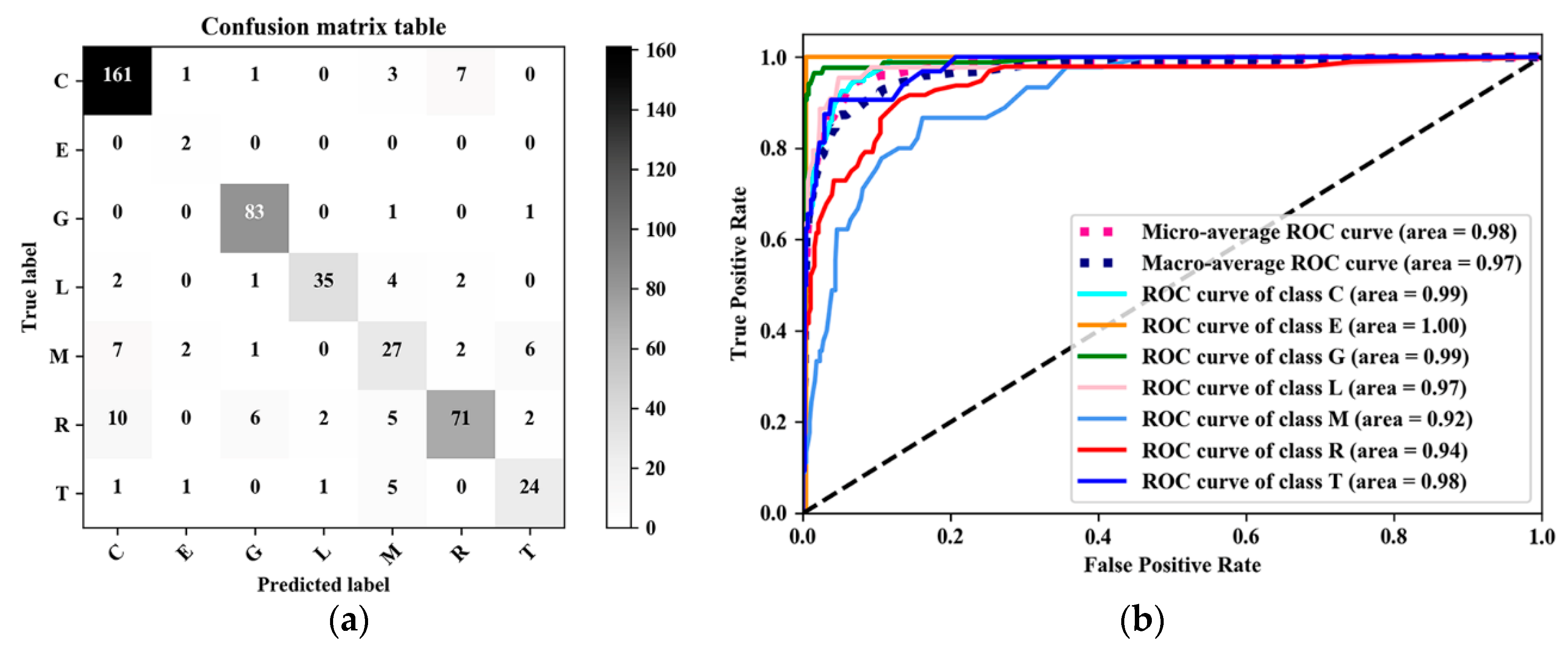
It has been an increasingly important issue recently to conduct the urban functional zones classification because it could provide a good reference for urban planners and decision makers to monitor the changes of urban functional zones over space and time for making better plans and decisions. However, urban functional zones classification remains a challenge due to the complexity of urban systems and the limitation of datasets. Although many classification approaches have been used to distinguish between different urban functional zones based on various kinds of datasets, there is still room for improvement in terms of designing and employing more effective models for better accuracy in the field. Newly developed machine learning classifier XGBoost has shown its high efficiency and effectiveness in many applications. However, it has not been tested and utilized in urban functional zones classification. Hence, in this study, the XGBoost model was employed, tested, and compared with other commonly used classification models to classify a variety of urban functional zones in the case study of Yuzhong District, Chongqing, China. In these successful experiments, the XGBoost model was found to be the best among all these commonly used models tested in this research, with the highest accuracy of 88.05%. The results could explicitly demonstrate that the XGBoost model could effectively be applied in urban functional zones classification through the combination of physical and socioeconomic features extracted from high-resolution satellite images and multi-source geospatial data, respectively. In this study, ensemble classifiers, such as XGBoost and Random Forest, have also shown a promising classification performance compared to other kinds of state-of-the-art classifiers. In addition, although XGBoost is a highly sophisticated algorithm, the model is still quite straightforward to use and is able to perform better than Random Forest and the other tested models based on accuracy, confusion matrix, ROC curves, and AUC values in this case study. This might be due to the following aspects: First, XGBoost is a regularized boosting technique and allows users to define custom optimization objectives and evaluation criteria, which is of high flexibility as well as able to reduce overfitting. Second, XGBoost is also able to handle missing values, which could decrease the uncertainty. Furthermore, Random Forest model ranks the second of all these tested models in the case study. As a tree-based model, the Decision Tree has also performed well, but less accurate than XGBoost and Random Forest models, respectively. Surprisingly, Multinomial Logistic Regression, as the most commonly used and simplest model, shows an accuracy of 70.86%, which is even better than SVM and K-Nearest Neighbors models in this study. SVM, although proved to be efficient in previous studies [26,44], only achieved an accuracy of 67.71% in this case study, which is less than most of the classification model tested in this study. The K-Nearest Neighbors model performed worst in both accuracy and classification separability in this study.

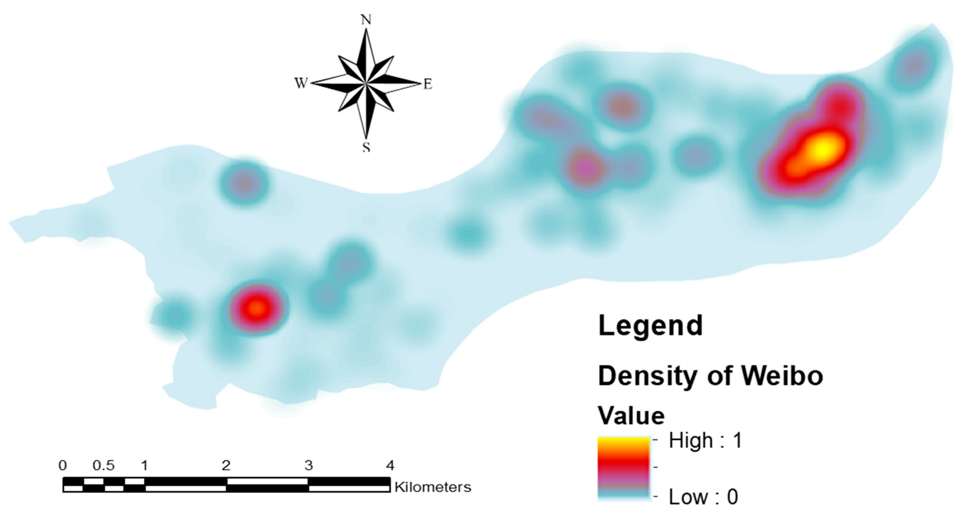
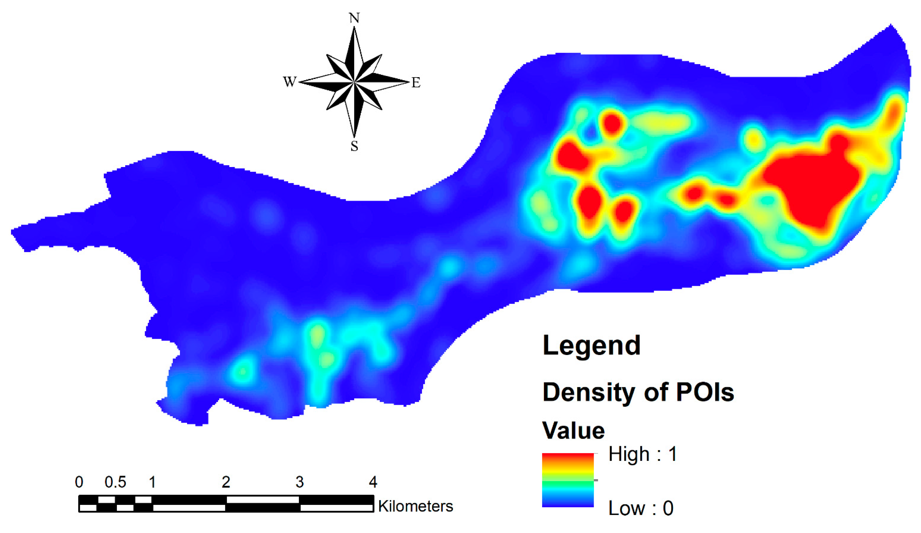
The success of our comparison between these models could be a good reference to other case studies in urban functional zones classification or even other applications of classifications. Furthermore, as the extension of our current research, more efforts will be put into the temporal dimension of urban functional zones classification, which requires even more efficient classification models or even integration of high-performance computation. In addition, in this research, the sample size was set to be 100 m by 100 m given the data availability and the size of the research area. However, the scale may also matter in the performance of these models, we would like to continue our research on this direction in the future. On the other hand, our case study based on multi-source geospatial datasets has also revealed the value of nighttime light imagery, social media datasets, POI datasets, and Baidu Heat Map to the recognition of urban functional zones. Of course, more geospatial datasets, especially social sensing datasets, are also worth exploring, which will also be one direction of our future research.

Last but not least, there are also a few limitations in this research. First, there exist some uncertainties on these multi-source geospatial data collected. Given that it applies to all these models, the influence on the results of our study could be ignored. Second, considering the computation intensity, the parameters calibration in this research could also be improved for possibly more precise results. These aspects will be addressed in our future research.

References

1. Zhang, X.; Du, S.; Wang, Q. Hierarchical semantic cognition for urban functional zones with VHR satellite images and POI data. ISPRS J. Photogramm. Remote Sens. 2017, 132, 170–184. [Google Scholar] [CrossRef]
2. Long, Y.; Shen, Z. Discovering functional zones using bus smart card data and points of interest in Beijing. In Geospatial Analysis to Support Urban Planning in Beijing; Springer: Berlin/Heidelberg, Germany, 2015; pp. 193–217. [Google Scholar]
3. Zhang, X.; Du, S. A linear dirichlet mixture model for decomposing scenes: Application to analyzing urban functional zonings. Remote Sens. Environ. 2015, 169, 37–49. [Google Scholar] [CrossRef]
4. Gao, S.; Janowicz, K.; Couclelis, H. Extracting urban functional regions from points of interest and human activities on location-based social networks. Trans. GIS 2017, 21, 446–467. [Google Scholar] [CrossRef]
5. Yuan, N.J.; Zheng, Y.; Xie, X.; Wang, Y.; Zheng, K.; Xiong, H. Discovering urban functional zones using latent activity trajectories. IEEE Trans. Knowl. Data Eng. 2015, 27, 712–725. [Google Scholar] [CrossRef]
6. Qiao, K.; Zhu, W.; Hu, D.; Hao, M.; Chen, S.; Cao, S. Examining the distribution and dynamics of impervious surface in different function zones in Beijing. J. Geogr. Sci. 2018, 28, 669–684. [Google Scholar] [CrossRef]
7. Tian, G.; Wu, J.; Yang, Z. Spatial pattern of urban functions in the Beijing metropolitan region. Habitat Int. 2010, 34, 249–255. [Google Scholar] [CrossRef]
8. Yao, Z.; Fu, Y.; Liu, B.; Hu, W.; Xiong, H. Representing Urban Functions through Zone Embedding with Human Mobility Patterns. In Proceedings of the Twenty-Seventh International Joint Conference on Artificial Intelligence, Stockholm, Sweden, 13–19 July 2018; pp. 3919–3925. [Google Scholar]
9. Rhinane, H.; Hilali, A.; Berrada, A.; Hakdaoui, M. Detecting slums from SPOT data in Casablanca Morocco using an object based approach. J. Geogr. Inf. Syst. 2011, 3, 217. [Google Scholar] [CrossRef]
10. Steeves, J.K.; Humphrey, G.K.; Culham, J.C.; Menon, R.S.; Milner, A.D.; Goodale, M. Behavioral and neuroimaging evidence for a contribution of color and texture information to scene classification in a patient with visual form agnosia. J. Cogn. Neurosci. 2004, 16, 955–965. [Google Scholar] [CrossRef]
11. Liu, Y.; Liu, X.; Gao, S.; Gong, L.; Kang, C.; Zhi, Y.; Chi, G.; Shi, L. Social sensing: A new approach to understanding our socioeconomic environments. Ann. Assoc. Am. Geogr. 2015, 105, 512–530. [Google Scholar] [CrossRef]
12. Elvidge, C.D.; Baugh, K.; Zhizhin, M.; Hsu, F.C.; Ghosh, T. VIIRS night-time lights. Int. J. Romote Sens. 2017, 38, 5860–5879. [Google Scholar] [CrossRef] [Green Version]
13. Aubrecht, C.; León Torres, J.A. Evaluating Multi-Sensor Nighttime Earth Observation Data for Identification of Mixed vs. Residential Use in Urban Areas. Remote Sens. 2016, 8, 114. [Google Scholar] [CrossRef]
14. Ratti, C.; Frenchman, D.; Pulselli, R.M.; Williams, S. Mobile landscapes: Using location data from cell phones for urban analysis. Environ. Plan. B Urban Anal. City Sci. 2006, 33, 727–748. [Google Scholar] [CrossRef]
15. Endo, Y.; Toda, H.; Nishida, K.; Ikedo, J. Classifying spatial trajectories using representation learning. Int. J. Data Sci. Anal. 2016, 2, 107–117. [Google Scholar] [CrossRef] [Green Version]
16. Crooks, A.; Pfoser, D.; Jenkins, A.; Croitoru, A.; Stefanidis, A.; Smith, D.; Karagiorgou, S.; Efentakis, A.; Lamprianidis, G. Crowdsourcing urban form and function. Int. J. Geogr. Inf. Sci. 2015, 29, 720–741. [Google Scholar] [CrossRef]
17. Jäppinen, S.; Toivonen, T.; Salonen, M. Modelling the potential effect of shared bicycles on public transport travel times in Greater Helsinki: An open data approach. Appl. Geogr. 2013, 43, 13–24. [Google Scholar] [CrossRef]
18. Bakillah, M.; Liang, S.; Mobasheri, A.; Jokar Arsanjani, J.; Zipf, A. Fine-resolution population mapping using OpenStreetMap points-of-interest. Int. J. Geogr. Inf. Sci. 2014, 28, 1940–1963. [Google Scholar] [CrossRef]
19. Yao, Y.; Li, X.; Liu, X.; Liu, P.; Liang, Z.; Zhang, J.; Mai, K. Sensing spatial distribution of urban land use by integrating points-of-interest and Google Word2Vec model. Int. J. Geogr. Inf. Sci. 2017, 31, 825–848. [Google Scholar] [CrossRef]
20. Jiang, S.; Alves, A.; Rodrigues, F.; Ferreira, J., Jr.; Pereira, F.C. Mining point-of-interest data from social networks for urban land use classification and disaggregation. Comput. Environ. Urban Syst. 2015, 53, 36–46. [Google Scholar] [CrossRef] [Green Version]
21. Yuan, J.; Zheng, Y.; Xie, X. Discovering regions of different functions in a city using human mobility and POIs. In Proceedings of the 18th ACM SIGKDD International Conference on Knowledge Discovery and Data Mining, Beijing, China, 12–16 August 2012; pp. 186–194. [Google Scholar]
22. Pei, T.; Sobolevsky, S.; Ratti, C.; Shaw, S.-L.; Li, T.; Zhou, C. A new insight into land use classification based on aggregated mobile phone data. Int. J. Geogr. Inf. Sci. 2014, 28, 1988–2007. [Google Scholar] [CrossRef] [Green Version]
23. Zhan, X.; Ukkusuri, S.V.; Zhu, F. Inferring urban land use using large-scale social media check-in data. Netw. Spat. Econ. 2014, 14, 647–667. [Google Scholar] [CrossRef]
24. Wieland, M.; Pittore, M. Performance evaluation of machine learning algorithms for urban pattern recognition from multi-spectral satellite images. Remote Sens. 2014, 6, 2912–2939. [Google Scholar] [CrossRef]
25. Yang, C.; Wu, G.; Ding, K.; Shi, T.; Li, Q.; Wang, J. Improving Land Use/Land Cover Classification by Integrating Pixel Unmixing and Decision Tree Methods. Remote Sens. 2017, 9, 1222. [Google Scholar] [CrossRef]
26. Mantero, P.; Moser, G.; Serpico, S.B. Partially supervised classification of remote sensing images through SVM-based probability density estimation. IEEE Trans. Geosci. Remote Sens. 2005, 43, 559–570. [Google Scholar] [CrossRef]
27. Zhang, Y.; Li, Q.; Huang, H.; Wu, W.; Du, X.; Wang, H. The combined use of remote sensing and social sensing data in fine-grained urban land use mapping: A case study in Beijing, China. Remote Sens. 2017, 9, 865. [Google Scholar] [CrossRef]
28. De Fries, R.; Hansen, M.; Townshend, J.; Sohlberg, R. Global land cover classifications at 8 km spatial resolution: The use of training data derived from Landsat imagery in decision tree classifiers. Int. J. Remote Sens. 1998, 19, 3141–3168. [Google Scholar] [CrossRef]
29. Mountrakis, G.; Im, J.; Ogole, C. Support vector machines in remote sensing: A review. ISPRS J. Photogramm. Remote Sens. 2011, 66, 247–259. [Google Scholar] [CrossRef]
30. Huang, C.; Davis, L.; Townshend, J. An assessment of support vector machines for land cover classification. Int. J. Remote Sens. 2002, 23, 725–749. [Google Scholar] [CrossRef]
31. Liu, X.; He, J.; Yao, Y.; Zhang, J.; Liang, H.; Wang, H.; Hong, Y. Classifying urban land use by integrating remote sensing and social media data. Int. J. Geogr. Inf. Sci. 2017, 31, 1675–1696. [Google Scholar] [CrossRef]
32. Palczewska, A.; Palczewski, J.; Robinson, R.M.; Neagu, D. Interpreting random forest classification models using a feature contribution method. In Integration of Reusable Systems; Springer: Berlin/Heidelberg, Germany, 2014; pp. 193–218. [Google Scholar]
33. Gislason, P.O.; Benediktsson, J.A.; Sveinsson, J.R. Random forests for land cover classification. Pattern Recogn. Lett. 2006, 27, 294–300. [Google Scholar] [CrossRef]
34. Rodriguez-Galiano, V.F.; Ghimire, B.; Rogan, J.; Chica-Olmo, M.; Rigol-Sanchez, J.P. An assessment of the effectiveness of a random forest classifier for land-cover classification. ISPRS J. Photogramm. Remote Sens. 2012, 67, 93–104. [Google Scholar] [CrossRef]
35. Ghimire, B.; Rogan, J.; Miller, J. Contextual land-cover classification: Incorporating spatial dependence in land-cover classification models using random forests and the Getis statistic. Remote Sens. Lett. 2010, 1, 45–54. [Google Scholar] [CrossRef]
36. Xiao, Z.; Wang, Y.; Fu, K.; Wu, F. Identifying different transportation modes from trajectory data using tree-based ensemble classifiers. Int. J. Geo-Inf. 2017, 6, 57. [Google Scholar] [CrossRef]
37. Li, X.; Li, D.; Xu, H.; Wu, C. Intercalibration between DMSP/OLS and VIIRS night-time light images to evaluate city light dynamics of Syria’s major human settlement during Syrian Civil War. Int. J. Remote Sens. 2017, 38, 5934–5951. [Google Scholar] [CrossRef]
38. Jackson, J.M.; Liu, H.; Laszlo, I.; Kondragunta, S.; Remer, L.A.; Huang, J.; Huang, H.C. Suomi-NPP VIIRS aerosol algorithms and data products. J. Geophys. Res. Atmos. 2013, 118, 12673–612689. [Google Scholar] [CrossRef]
39. Li, X.; Chen, X.; Zhao, Y.; Xu, J.; Chen, F.; Li, H. Automatic intercalibration of night-time light imagery using robust regression. Remote Sens. Lett. 2013, 4, 45–54. [Google Scholar] [CrossRef]
40. Nip, J.Y.; Fu, K.-W. Challenging official propaganda? Public opinion leaders on Sina Weibo. China Q. 2016, 225, 122–144. [Google Scholar] [CrossRef]
41. Ye, Z.; Chen, Y.; Zhang, L. The Analysis of Space Use around Shanghai Metro Stations Using Dynamic Data from Mobile Applications. Transp. Res. Procedia 2017, 25, 3147–3160. [Google Scholar] [CrossRef]
42. Greene, W.H. Econometric Analysis; Pearson Education India: Chennai, India, 2003. [Google Scholar]
43. Mingqin, H.; Tao, J.; Weizheng, Z.; Shouyin, D.; Wenhu, L. Landuse information extraction in Qingdao based on decision tree classification. In Proceedings of the 2010 3rd International Congress on Image and Signal Processing (CISP), Yantai, China, 16–18 October 2010; pp. 2194–2197. [Google Scholar]
44. Deng, H.; Runger, G.; Tuv, E. Artificial Neural Networks and Machine Learning—ICANN 2011; Springer: Berlin/Heidelberg, Germany, 2011. [Google Scholar]
45. Cao, X.; Chen, J.; Imura, H.; Higashi, O. A SVM-based method to extract urban areas from DMSP-OLS and SPOT VGT data. Remote Sens. Environ. 2009, 113, 2205–2209. [Google Scholar] [CrossRef]
46. Vapnik, V. The Nature of Statistical Learning Theory; Springer: Berlin/Heidelberg, Germany, 2013. [Google Scholar]
47. Breiman, L. Random forests. Mach. Learn. 2001, 45, 5–32. [Google Scholar] [CrossRef]
48. Dong, H.; Xu, X.; Wang, L.; Pu, F. Gaofen-3 PolSAR image classification via XGBoost and polarimetric spatial information. Sensors 2018, 18, 611. [Google Scholar] [CrossRef]
49. Chen, T.; Guestrin, C. Xgboost: A scalable tree boosting system. In Proceedings of the 22nd ACM SIGKDD International Conference on Knowledge Discovery and Data Mining, San Francisco, CA, USA, 13–17 August 2016; pp. 785–794. [Google Scholar]
50. Hajian-Tilaki, K. Receiver operating characteristic (ROC) curve analysis for medical diagnostic test evaluation. Casp. J. Intern. Med. 2013, 4, 627. [Google Scholar]
51. Tu, W.; Cao, J.; Yue, Y.; Shaw, S.-L.; Zhou, M.; Wang, Z.; Chang, X.; Xu, Y.; Li, Q. Coupling mobile phone and social media data: A new approach to understanding urban functions and diurnal patterns. Int. J. Geogr. Inf. Sci. 2017, 31, 2331–2358. [Google Scholar] [CrossRef]
52. Chongqing Urban and Rural Master Urban Plan for 2007–2020; Chongqing Government: Chongqing, China, 2011.
53. Jiang, S.; Pang, G.; Wu, M.; Kuang, L. An improved K-nearest-neighbor algorithm for text categorization. Expert Syst. Appl. 2012, 39, 1503–1509. [Google Scholar] [CrossRef]
Figure 1. Yuzhogng District, Chongqing Municipality, China.
Sustainability 11 00660 g001
Figure 2. Density of Weibo in the study area.
Sustainability 11 00660 g002
Figure 3. Density of POI data in the study area.
Sustainability 11 00660 g003
Figure 4. Baidu Heat Map of the study area.
Sustainability 11 00660 g004
Figure 5. Research framework.
Sustainability 11 00660 g005
Figure 6. Yuzhong District with urban functional zones labels.
Sustainability 11 00660 g006
Figure 7. The count of urban functional zones grids.
Sustainability 11 00660 g007
Figure 8. The Multinomial Logistic Regression model: (a) the confusion matrix; (b) the receiver operating characteristics (ROC) curve (area represents area under the curve (AUC) value).
Sustainability 11 00660 g008
Figure 9. The k-nearest neighbor (KNN) model: (a) the confusion matrix; and (b) the ROC curve (area represents AUC value).
Sustainability 11 00660 g009
Figure 10. The Decision Tree model: (a) the confusion matrix; and (b) the ROC curve (area represents AUC value).
Sustainability 11 00660 g010
Figure 11. The SVM model: (a) the confusion matrix; and (b) the ROC curve (area represents AUC value).
Sustainability 11 00660 g011
Figure 12. The Random Forest model: (a) the confusion matrix; (b) the ROC curve (area represents AUC value).
Sustainability 11 00660 g012
Figure 13. The XGBoost model: (a) the confusion matrix; and (b) the ROC curves (area represents AUC value).
Sustainability 11 00660 g013